Pricing Variable Annuity Guarantees in a Local Volatility framework

Abstract

In this paper, we study the price of Variable Annuity Guarantees, especially of Guaranteed Annuity Options (GAO) and Guaranteed Minimum Income Benefit (GMIB), and this in the settings of a derivative pricing model where the underlying spot (the fund) is locally governed by a geometric Brownian motion with local volatility, while interest rates follow a Hull-White one-factor Gaussian model. Notwithstanding the fact that in this framework, the local volatility depends on a particularly complicated expectation where no closed-form expression exists and it is neither directly related to European call prices or other liquid products, we present in this contribution different methods to calibrate the local volatility model. We further compare Variable Annuity Guarantee prices obtained in three different settings, namely the local volatility, the stochastic volatility and the constant volatility models all combined with stochastic interest rates and show that an appropriate volatility modelling is important for these long-dated derivatives. More precisely, we compare prices of GAO, GMIB Rider and barrier types GAO obtained by using local volatility, stochastic volatility and constant volatility models.

1 Introduction

Variable Annuities are insurance contracts that propose a guaranteed return at retirement often higher than the current market rate and therefore they have become a part of the retirement plans of many people. Variable Annuity products are generally based on an investment in a mutual fund composed of stocks and bonds (see for example Gao GaoJin and Pelsser and Schrager Pelsser2 ) and they offer a range of options to give minimum guarantees and protect against negative equity movement. One of the most popular type of Variable Annuity Guarantees in Japan and North America is the Guaranteed Minimum Income Benefit (GMIB). At her retirement date, a GMIB policyholder will have the right to choose between the fund value at that time or (life) annuity payments based on the initial fund value at a fixed guarantee rate. Similar products are available in Europe under the name Guaranteed Annuity Options (GAO). Many authors have already studied the pricing and hedging of GMIBs and GAOs assuming a geometric Brownian motion and a constant volatility for the fund value (see for example Boyle and Hardy Boyle01 ; Boyle , Ballotta and Haberman Ballotta , Pelsser Pelsser , Biffis and Millossovich Biffis , Marshall et al. Hardy2 , Chu and Kwok Chu_Kwok ).

GAO and GMIB can be considered as long-dated options since their maturity is based on the retirement date. When pricing long-dated derivatives, it is highly recommended that the pricing model used to evaluate and hedge the products takes into account the stochastic behavior of the interest rates as well as the stochastic behavior of the fund. Furthermore, the volatility of the fund can have a significant impact and should not be neglected. It has been shown in Boyle that the value of the fund as well as the interest rates and the mortality assumptions influence strongly the cost of these guarantees. Some authors consider the evolution of mortality stochastic as well (see for example (Ballotta, ) and Biffis ). In van_Haastrecht_GAO , van Haastrecht et al. have studied the impact of the volatility of the fund on the price of GAO by using a stochastic volatility approach.

Another category of models able to fit the vanilla market implied volatilities are local volatility models introduced by Derman and Kani and Dupire in 1994 in resp. Derman and Dupire and recently extended to a stochastic interest rate framework by, among others, Atlan Atlan , Piterbarg Piterbarg2005 and Deelstra and Rayee Deelstra-Rayee . The main advantage of local volatility models is that the volatility is a deterministic function of the equity spot and time which avoids the problem of working in incomplete markets in comparison with stochastic volatility models. Therefore local volatility models are more appropriate for hedging strategies. The local volatility function is expressed in terms of implied volatilities or market call prices and the calibration is done on the whole implied volatility surface directly. Consequently, local volatility models usually capture more precisely the surface of implied volatilities than stochastic volatility models.

Stochastic volatility models have the advantage that it is possible to derive closed-form solutions for some European derivatives. In (van_Haastrecht_GAO, ), van Haastrecht et al. have derived closed-form formulae for GAO prices in the Schöbel and Zhu stochastic volatility model combined with Hull and White stochastic interest rates. However, the GMIB Rider, one of the popular products traded by insurance companies in North America (see GMIB ) has a more complicated payoff than a pure GAO and therefore there exists no closed-form solution for the price of a GMIB Rider, even not in the Schöbel and Zhu stochastic volatility model. The only way to evaluate a GMIB Rider is by using numerical approaches like for example Monte Carlo simulations.

In this paper, we study the prices of GAO, GMIB Riders and barrier type GAOs in the settings of a two-factor pricing model where the equity (fund) is locally governed by a geometric Brownian motion with a local volatility, while interest rates follow a Hull-White one-factor Gaussian model. In this framework, the local volatility expression contains an expectation for which no closed-form expression exists and which is unfortunately not directly related to European call prices or other liquid products. Its calculation can be done by numerical integration methods or Monte Carlo simulations. An alternative approach is to calibrate the local volatility from stochastic volatility models by establishing links between local and stochastic volatility. A last calibration approach presented in this paper is by adjusting the tractable local volatility surface coming from a deterministic interest rates framework.

Furthermore, we compare Variable Annuity Guarantee prices obtained in three different settings, namely, the local volatility, the stochastic volatility and the constant volatility models all in the settings of stochastic interest rates. We show that using a non constant volatility for the volatility of the equity fund value can have significant impact on the value of these Variable Annuity Guarantees and that the impact generated by a local volatility model is not equivalent to the one generated by a stochastic volatility model, even if both are calibrated to the same market data.

This paper is organized as follows: Section 2 introduces the local volatility model with stochastic interest rates we use in this paper to price Variable Annuity Guarantees. In Section 3, we present different approaches for the calibration of the local volatility function. In Subsection 3.1, we derive an analytical expression for the local volatility. In Subsection 3.2, we explain in detail the different steps for applying a Monte Carlo method in the calibration procedure. Next, in Subsection 3.3 we give a link between the local volatility function derived in a two-factor local volatility model and the tractable one coming from the simple one-factor Gaussian model. Finally, in Subsection 3.4, a link is given between the stochastic volatility model and the local volatility model in a stochastic interest rates framework. In Section 4, we present the three types of Variable Annuity Guarantees we study in this paper, namely, the GAO, the GMIB Rider and barrier types GAO. In Subsection 4.1, we present the GAO, then, in Subsection 4.2, we define a GMIB Rider and finally in Subsection 4.3, we study two types of barrier GAO. Section 5 is devoted to numerical results. In Subsection 5.1, we present the calibration procedure for the Hull and White parameters and the calibration of the local volatility with respect to the vanilla market. In Subsection 5.2, we compare local volatility surfaces obtained in a stochastic and in a constant interest rates framework. Subsection 5.3, 5.4 and 5.5 investigate how the local volatility model behaves when pricing GAO, GMIB Rider and barrier types GAO (respectively) with respect to the Schöbel-Zhu Hull-White stochastic volatility model and the Black-Scholes Hull-White model. Conclusions are given in Section 6.

2 The local volatility model with stochastic interest rates

In this paper we consider a two-factor model where the volatility of the fund value $S$ is a deterministic function of both time and the fund itself. This function is known as “local volatility”. In this model, the fund value $S$ is governed by the following dynamics

$$dS(t)=(r(t)-q)S(t)dt+\sigma(t,S(t))S(t)dW^{Q}_{S}(t),$$ (1)

where interest rates follow a Hull-White one-factor Gaussian model (HullandWhite, ) defined by the Ornstein-Uhlenbeck processes.

$$dr(t)=[\theta(t)-\alpha(t)r(t)]dt+\sigma_{r}(t)dW^{Q}_{r}(t),$$ (2)

where $\theta(t),\sigma_{r}(t)$ and $\alpha(t)$ are deterministic functions of time. Equations (1) and (2) are expressed under the risk-neutral measure $Q$. We have chosen the very popular Hull-White model since it is a tractable nontrivial interest rate model, allowing closed-form solutions for many derivatives which is useful for the calibration.

We assume that the dynamics of the fund and the interest rates are linked by the following correlation structure:

$$E^{Q}[dW^{Q}_{S}dW^{Q}_{r}]=\rho_{Sr}dt.$$ (3)

In the following we will denote this model by LVHW since it combines a local volatility model with a Hull-White one-factor Gaussian model. When $\sigma(t,S(t))$ equals a constant, this model reduces to the Black-Scholes Hull-White model, denoted by BSHW.

3 Calibration

Before using a model to price any derivatives, practitioners are used to calibrate it on the vanilla market. The calibration consists of determining all parameters present in the different stochastic processes which define the model in such a way that all European option prices derived in the model are as consistent as possible with the corresponding market ones. More precisely, they need a model which, after calibration, is able to price vanilla options such that the resulting implied volatilities match the market-quoted ones.

The calibration procedure for the LVHW model can be decomposed in three steps: (i) Parameters present in the Hull-White one-factor dynamics for the interest rates, namely $\theta(t),\alpha(t)$ and $\sigma_{r}(t)$, are chosen to match European swaptions. Methods for doing so are well developed in the literature (see for example (Brigo-Mercurio, )). (ii) The correlation coefficient $\rho_{Sr}$ is estimated from historical data. (iii) After these two steps, one has to find the local volatility function which is consistent with the implied volatility surface.

3.1 The local volatility function

In Deelstra-Rayee we derived the local volatility expression associated to a three-factor model by differentiating the expression of a European call price ($C(K,T)$) with respect to its strike $K$ and its maturity $T$. Following the same idea we can derive the local volatility expression associated to the two-factor model presented in Section 2. This leads to,

$$\sigma(T,K)=\sqrt{\frac{\frac{\partial C(K,T)}{\partial T}+qC(K,T)-qK\frac{\partial C(K,T)}{\partial K}+KP(0,T)\mathbf{E}^{Q_{T}}[r(T)\textbf{1}_{\{S(T)>K\}}]}{\frac{1}{2}K^{2}\frac{\partial^{2}C}{\partial K^{2}}}},$$ (4)

where $Q_{T}$ is the $T$-forward measure.

This local volatility function is not easy to calibrate with respect to the vanilla market since there is no immediate way to link the expectation term ($\mathbf{E}^{Q_{T}}[r(T)\textbf{1}_{\{S(T)>K\}}]$) with vanilla option prices or other liquid products. However, we present in this section three different methods to calibrate it.

Note that when assuming constant interest rates $(r=r(0))$, equation (4) reduces to the simple Dupire formula (see Dupire ) corresponding to the one-factor Gaussian case:

$$\sigma(T,K)=\sqrt{\frac{\frac{\partial C(K,T)}{\partial T}+(r-q)K\frac{\partial C(K,T)}{\partial K}+qC(K,T)}{\frac{1}{2}K^{2}\frac{\partial^{2}C(K,T)}{\partial K^{2}}}}.$$ (5)

Since the market often quotes options in terms of implied volatilities $\sigma_{imp}$ instead of option prices, it is more convenient to express the local volatility in terms of implied volatilities. The implied volatility of an option with price $C(K,T)$, is defined through the Black-Scholes formula ($C^{mkt}(K,T)=C^{BS}(K,T,\sigma_{imp})$) and therefore computing the derivatives of call prices through the chain rule and substituting in equation (5) leads to the following equation (see (Wilmott2, )),

$$\sigma(T,K) = \sqrt{\frac{Vega^{BS}(\frac{\sigma_{imp}}{2T}+\frac{\partial\sigma_{imp}}{\partial T}+(r-q)K\frac{\partial\sigma_{imp}}{\partial K})}{\frac{1}{2}K^{2}Vega^{BS}(\frac{1}{\sigma_{imp}K^{2}T}+\frac{2d_{+}}{\sigma_{imp}K\sqrt{T}}\frac{\partial\sigma_{imp}}{\partial K}+\frac{\partial^{2}\sigma_{imp}}{\partial K^{2}}+\frac{d_{+}d_{-}}{\sigma_{imp}}(\frac{\partial\sigma_{imp}}{\partial K})^{2})}}$$ (6)

$$= \sqrt{\frac{\sigma^{2}_{imp}+2T\sigma_{imp}\frac{\partial\sigma_{imp}}{\partial T}+2(r-q)KT\sigma_{imp}\frac{\partial\sigma_{imp}}{\partial K}}{(1+Kd_{+}\sqrt{T}\frac{\partial\sigma_{imp}}{\partial K})^{2}+K^{2}T\sigma_{imp}(\frac{\partial^{2}\sigma_{imp}}{\partial K^{2}}-d_{+}(\frac{\partial\sigma_{imp}}{\partial K})^{2}\sqrt{T})}},$$

with

$$d_{\pm}=\frac{log\frac{S(0)}{K}+(r-q\pm\frac{\sigma^{2}_{imp}}{2})T}{\sigma_{imp}\sqrt{T}},$$

$$\mathcal{N}(x)=\int_{-\infty}^{x}\frac{1}{\sqrt{2\pi}}e^{\frac{-z^{2}}{2}}dz,$$

$$Vega^{BS}=e^{-qT}S(0)\mathcal{N}^{\prime}(d_{+})\sqrt{T},$$

$$\mathcal{N}^{\prime}(x)=\frac{1}{\sqrt{2\pi}}e^{\frac{-x^{2}}{2}}.$$

Using the same approach, the local volatility expression (4) can be written in terms of implied volatilities $\sigma_{imp}$,

$$\sigma(T,K)=\sqrt{\frac{Vega^{BS}(\frac{\sigma_{imp}}{2T}+\frac{\partial\sigma_{imp}}{\partial T}-qK\frac{\partial\sigma_{imp}}{\partial K})+Kr(0)e^{-r(0)T}\mathcal{N}(d_{-})+KP(0,T)\mathbf{E}^{Q_{T}}[r(T)\textbf{1}_{\{S(T)>K\}}]}{\frac{1}{2}K^{2}Vega^{BS}(\frac{1}{\sigma_{imp}K^{2}T}+\frac{2d_{+}}{\sigma_{imp}K\sqrt{T}}\frac{\partial\sigma_{imp}}{\partial K}+\frac{\partial^{2}\sigma_{imp}}{\partial K^{2}}+\frac{d_{+}d_{-}}{\sigma_{imp}}(\frac{\partial\sigma_{imp}}{\partial K})^{2})}}.$$

3.2 The Monte Carlo approach

In this section we present a Monte Carlo approach for the calibration of the local volatility expression (4) or (LABEL:locvol_implied_C). More precisely, we use Monte Carlo simulations to calculate an approximation of the expectation $\mathbf{E}^{Q_{T}}[r(T)\textbf{1}_{\{S(T)>K\}}]$. Therefore we have to simulate interest rates $r(t)$ and the fund value $S(t)$ up to time $T$ starting from the actual interest rate $r(0)$ and fund value $S(0)$ respectively. Note that in the remainder of the paper we concentrate on the Hull and White model where $\alpha(t)=\alpha$ and $\sigma_{r}(t)=\sigma_{r}$ are positive constants. In HullandWhite1995b , Hull and White remarked that the future volatility structure implied by (2) are likely to be unrealistic in the sense that they do not conform to typical market shapes. We therefore assume, exactly as Hull and White in HullandWhite1994A , $\alpha(t)$ and $\sigma_{r}(t)$ as positive constants. In that case, one can exactly fit the market term structure of interest rates if the parameter $\theta(t)$ satisfies (see Brigo-Mercurio and HullandWhite1994A )

$$\theta(t)=\frac{\partial f^{mkt}(0,t)}{\partial T}+\alpha f^{mkt}(0,t)+\frac{\sigma_{r}^{2}}{2\alpha^{2}}(1-e^{-2\alpha t}),$$

where $f^{mkt}(0,t)$ denotes the market instantaneous forward rate at time 0 for the maturity $t$ and where $\frac{\partial f^{mkt}}{\partial T}$ denotes partial derivatives of $f^{mkt}$ with respect to its second argument.

Since the expectation $\mathbf{E}^{Q_{T}}[r(T)\textbf{1}_{\{S(T)>K\}}]$ is expressed under the measure $Q_{T}$, we use the dynamics of $S(t)$ and $r(t)$ under that measure, namely,

$$dS(t)=(r(t)-q-\sigma(t,S(t))\sigma_{r}b(t,T)\rho_{Sr})S(t)dt+\sigma(t,S(t))S(t)dW^{Q_{T}}_{S}(t),$$ (8)

$$dr(t)=[\theta(t)-\alpha r(t)-\sigma^{2}_{r}(t)b(t,T)]dt+\sigma_{r}dW^{Q_{T}}_{r}(t),$$ (9)

where $b(t,T)=\frac{1}{\alpha}(1-e^{-\alpha(T-t)})$.

Following the Monte Carlo principle, we simulate $n$ times (i.e. $n$ scenarios) the stochastic variables $r(t)$ and $S(t)$ up to time $T$, using $\Delta t$ as time step of discretization and applying an Euler scheme for example. Therefore, the expectation is approximated by:

$$\mathbf{E}^{Q_{T}}[r(T)\textbf{1}_{\{S(T)>K\}}]\cong\frac{1}{n}\sum_{i=1}^{n}r_{i}(T)\textbf{1}_{\{S_{i}(T)>K\}},$$ (10)

where $i$ corresponds to the $i^{th}$-scenario, $i=1,...,n$.

Note that with a well-known change of variable, one can remove the need to calculate $\theta(t)$. The idea is to rewrite the stochastic interest rates as a sum of a stochastic and a deterministic part (see (Brigo-Mercurio, )):

$$r(t)=x(t)+\overline{x}(t),$$ (11)

where the stochastic part obeys the following dynamics:

$$dx(t)=-(\alpha x(t)+\sigma^{2}_{r}(t)b(t,T))dt+\sigma_{r}(t)dW^{Q_{T}}_{r}(t)$$ (12)

and where the deterministic part obeys the dynamics :

$$d\overline{x}(t)=(\theta(t)-\alpha\overline{x}(t))dt,$$ (13)

which yields to (see (Brigo-Mercurio, )):

$$\overline{x}(t)=f^{mkt}(0,t)+\frac{\sigma_{r}^{2}}{2\alpha^{2}}(1-e^{-\alpha t})^{2}.$$

To illustrate the algorithm, consider the case of using an Euler scheme for equations (8) and (12),

$$S(t_{k}+1) = S(t_{k})+(r(t_{k})-q-\sigma(t_{k},S(t_{k}))\sigma_{r}b(t_{k},T)\rho_{Sr})S(t_{k})\Delta t+\sigma(t_{k},S(t_{k}))S(t_{k})\sqrt{\Delta t}Z_{S},$$

$$x(t_{k+1}) = x(t_{k})-[\alpha x(t_{k})+\sigma^{2}_{r}b(t_{k},T)]\Delta t+\sigma_{r}\sqrt{\Delta t}[\rho_{Sr}Z_{S}+\sqrt{1-\rho_{Sr}^{2}}Z_{r}],$$

$$r(t_{k+1}) = x(t_{k+1})+\overline{x}(t_{k+1}),$$ (14)

where

$$\overline{x}(t_{k})=f^{mkt}(0,t_{k})+\frac{\sigma_{r}^{2}}{2\alpha^{2}}(1-e^{-\alpha t_{k}})^{2}\ \text{and}\ b(t_{k},T)=\frac{1}{\alpha}(1-e^{-\alpha(T-t_{k})})$$

and $Z_{r}$ and $Z_{S}$ are two independent standard normal variables.

As one can see in equation (14), the local volatility function has to be known for the simulation of the path for $S(t)$ and $r(t)$. Consequently, the only possible way to work is forward in time. To begin, we have to determine the local volatility function at the first time step $T=T_{1}$ for all strikes $K$. At this first step we assume that the initial local volatility is equal to the deterministic local volatility given by equation (5). Note that this local volatility is directly obtained by using market data (see equation (6)). More precisely, by this choice, we assume that for a “small time period”, interest rates are constant and in this case, the local volatility expression (4) reduces to (5). Knowing that local volatility function, $S(T_{1})$ and $r(T_{1})$ can be simulated. Then, the expectation $\mathbf{E}^{Q_{T_{1}}}[r(T_{1})\textbf{1}_{\{S(T_{1})>K\}}]$ can be computed for all $K$ by using:

$$\mathbf{E}^{Q_{T_{1}}}[r(T_{1})\textbf{1}_{\{S(T_{1})>K\}}]\cong\frac{1}{n}\sum_{i=1}^{n}r_{i}(T_{1})\textbf{1}_{\{S_{i}(T_{1})>K\}}.$$ (15)

At this step we are able to build the local volatility function at time $T_{1}$, $\sigma^{2}(T_{1},K)$ for all strikes $K$. Following the same procedure we can easily calibrate the local volatility at time $T_{2}$ by using the local volatility obtained at time $T_{1}$ and also the simulated paths until time $T_{1}$. Following this procedure we are able to generate the local volatility expression up to a final date $T=T_{k}$.

3.3 Comparison between local volatility with and without stochastic interest rates

Assuming that quantities $\mathbf{Cov}^{Q_{T}}[r(T),\textbf{1}_{\{S(T)>K\}}]$ are extractable from the market, it is possible to adjust the tractable Dupire local volatility function $\sigma_{1f}(T,K)$ coming from the one-factor Gaussian model (see equation (5)) in order to obtain the local volatility surface which takes into account the effects of stochastic interest rates $\sigma_{2f}(T,K)$ (i.e. equation (4)).

More precisely, the adjustment $\sigma_{2f}^{2}(T,K)-\sigma_{1f}^{2}(T,K)$ is given by

$$\sigma_{2f}^{2}(T,K)-\sigma_{1f}^{2}(T,K)=\frac{P(0,T)\mathbf{Cov}^{Q_{T}}[r(T),\textbf{1}_{\{S(T)>K\}}]}{\frac{1}{2}K\frac{\partial^{2}C}{\partial K^{2}}},$$ (16)

where $\mathbf{Cov}^{Q_{T}}(X,Y)$ represents the covariance between two stochastic variables X and Y with dynamics expressed in the $T$-forward measure $Q_{T}$.

3.4 Calibrating the local volatility by mimicking stochastic volatility models

In this subsection, we give the link between the local volatility model and a stochastic volatility one under the assumption that interest rates are stochastic in both models. This link gives a way to calibrate the local volatility from stochastic volatility models.

Consider the following risk neutral dynamics for the equity spot

$$dS(t)=(r(t)-q)S(t)dt+\gamma(t,\nu(t))S(t)dW^{Q}_{S}(t),$$ (17)

Common designs for the function $\gamma(t,\nu(t))$ are $\nu(t)$, $exp(\sqrt{\nu(t)})$ and $\sqrt{\nu(t)}$. The stochastic variable $\nu(t)$ is generally modelled by a Cox-Ingersoll-Ross (CIR) process (as for example the Heston model (heston, )) or if the function $\gamma(t,\nu(t))$ allows for negative values for the stochastic volatility $\nu(t)$, by an Ornstein-Uhlenbeck process (OU) (as for example the Schöbel and Zhu (SchobelandZhu, ) stochastic volatility model).

In (Atlan, ) and (Deelstra-Rayee, ), the authors have shown that if there exists a local volatility such that the one-dimensional probability distribution of the equity spot with the diffusion (1) is the same as the one of the equity spot with dynamics (17) for every time $t$ when assuming that the risk neutral probability measure $Q$ used in the stochastic and the local volatility framework is the same, then the local volatility function $\sigma(t,S(t)=K)$ is given by the square root of the conditional expectation under the $t$-forward measure of the instantaneous equity stochastic spot volatility at the future time $t$, conditional on the equity spot level $S(t)$ being equal to $K$:

$$\sigma(t,K)=\sqrt{\mathbf{E}^{Q_{t}}[\gamma^{2}(t,\nu(t))\mid S(t)=K]}.$$ (18)

Remark 1

If we assume independence between the spot equity and its volatility, the local volatility function is given by $\sigma(T,K)=\sqrt{\mathbf{E}^{Q_{T}}[\gamma^{2}(T,\nu(T))]}$. Depending on the dynamics chosen for the stochastic variable $\nu(t)$, it is sometimes possible to derive closed-form solutions for this expectation. For example consider the following stochastic volatility model where interest rates have Hull and White dynamics and with Schöbel and Zhu dynamics for the equity spot volatility ($\nu(t)$):

$$dS(t)=(r(t)-q)S(t)dt+\nu(t)S(t)dW^{Q}_{S}(t),$$ (19)

$$dr(t)=[\theta(t)-\alpha r(t)]dt+\sigma_{r}dW^{Q}_{r}(t),$$ (20)

$$d\nu(t)=\kappa[\psi-\nu(t)]\ dt+\tau dW^{Q}_{\nu}(t).$$ (21)

In this case, we have a closed-form solution for the local volatility function given by

$$\sigma(T,K)=\sqrt{\left(\nu(0)e^{-\kappa T}+(\psi-\frac{\rho_{r\nu}\sigma_{r}\tau}{\alpha\kappa})(1-e^{-\kappa T})+\frac{\rho_{r\nu}\sigma_{r}\tau}{\alpha(\alpha+\kappa))}(1-e^{-(\alpha+\kappa)T})\right)^{2}+\frac{\tau^{2}}{2\kappa}(1-e^{-2\kappa T})}.$$

4 Variable Annuity Guarantees

In this section we present three different Variable Annuity products and in section 5.3, we discuss the price of all these products using local, stochastic and constant volatility models. We first define in Subsection 4.1 the Guaranteed Annuity Option and afterwards we define in Subsection 4.2 the Guaranteed Minimum Income Benefit (Rider). This last product has the particularity to be strongly dependent upon the path of the fund value. Finally, in subsection 4.3, we study two barrier type GAOs with a strong dependence upon the path of the interest rates.

4.1 Guaranteed Annuity Options

Consider an $x$ year policyholder who disposes at time $T$ of the payout of his capital policy which corresponds to an amount of money $S(T)$. A Guaranteed Annuity Option gives to the policyholder the right to choose either an annual payment of $S(T)g$ where $g$ is a fixed rate called the Guaranteed Annuity rate or a cash payment equal to the equity fund value $S(T)$ at time $T$ which can be considered as an annual payment of $S(T)r_{x}(T)$, with $r_{x}(T)$ being the market annuity payout rate defined by $r_{x}(T)=\frac{1}{\ddot{a}_{x}(T)}$ with $\ddot{a}_{x}(T)=\overset{\omega-(x+T)}{\underset{n=0}{\sum}}\phantom{.}_{n}p_{x+T}P(T,T+n)$ where $\omega$ is the largest survival age, $P(T,T+n)$ is the zero-coupon bond at time $T$ maturing at $T+n$ and $\phantom{.}{}_{n}p_{x+T}$ is the probability that the remaining lifetime of the policyholder at time $T$ is strictly greater than $n$. At time $T$ the value of the GAO is given by

$$V(T) = max(S(T)g\ddot{a}_{x}(T),S(T))$$ (22)

$$= S(T)+gS(T)max((\sum_{n=0}^{\omega-(x+T)}\phantom{.}{}_{n}p_{x+T}\ P(T,T+n))-K,0),$$ (23)

where $K=\frac{1}{g}$.

Assuming that the mortality risk is unsystematic and independent of the financial risk and applying the risk-neutral valuation procedure, we can write the value of a GAO entered by an $x$-year policyholder at time $t=0$ as

$$V(x,0,T) = E^{Q}[e^{-\int_{0}^{T}r(s)ds}V(T)1_{(\tau_{x}>T)}|\mathcal{F}_{0}]$$ (24)

$$= E^{Q}[e^{-\int_{0}^{T}r(s)ds}V(T)]E^{Q}[1_{(\tau_{x}>T)}]$$

$$= E^{Q}[e^{-\int_{0}^{T}r(s)ds}V(T)]\phantom{.}_{T}p_{x},$$

where $\tau_{x}$ is a random variable which represents the remaining lifetime of the policyholder. Substituting equation (23) in (24) leads to

$$V(x,0,T)=\phantom{.}_{T}p_{x}E^{Q}[e^{-\int_{0}^{T}r(s)ds}S(T)]+C(x,0,T).$$ (25)

where

$$C(x,0,T)=\phantom{.}_{T}p_{x}E^{Q}\left[e^{-\int_{0}^{T}r(s)ds}gS(T)[max((\sum_{n=0}^{\omega-(x+T)}\phantom{.}{}_{n}p_{x+T}P(T,T+n))-K,0)]\right].$$ (26)

Under the usual assumption of absence of arbitrage opportunities, the discounted value of the risky fund $e^{-\int_{0}^{T}r(s)ds}S(T)$ is a martingale under the risk neutral measure $Q$ and therefore the value of the GAO becomes

$$V(x,0,T)=\phantom{.}_{T}p_{x}S(0)+C(x,0,T).$$ (27)

The first term in equation (27) is a constant and therefore, in the literature, one studies generally only the second term $C(x,0,T)$. In Ballotta and van_Haastrecht_GAO , the authors define $C(x,0,T)$ as the GAO total value. In this paper we keep the same terminology. More precisely, in section 5.3, when we compare GAO total values obtained in different models, we compare values obtained for $C(x,0,T)$.

To derive analytical expressions for $C(x,0,T)$ in the Black-Scholes Hull-White and the Schöbel-Zhu Hull-White models it is more convenient to work under the measure $Q_{S}$ (where the numeraire is the fund value $S$), rather than under the risque neutral measure $Q$ (see Ballotta and van_Haastrecht_GAO ). By the density process $\xi_{T}=\frac{dQ_{S}}{dQ}|_{\mathcal{F}_{T}}=e^{-\int_{0}^{T}r(s)ds}\frac{S(T)}{S(0)}$ a new probability measure $Q_{S}$ equivalent to the measure $Q$ is defined, see e.g. Geman et al. Geman . Under this new measure $Q_{S}$, the $C(x,0,T)$ value becomes

$$C(x,0,T)=\phantom{.}_{T}p_{x}gS(0)E^{Q_{S}}[(\sum_{n=0}^{\omega-(x+T)}\phantom{.}{}_{n}p_{x+T}P(T,T+n)-K)^{+}].$$ (28)

Under $Q_{S}$ one has the following model dynamics

$$dS(t) = [r(t)-q+\sigma^{2}(t,S(t))]S(t)dt+\sigma(t,S(t))S(t)dW^{Q_{S}}_{S}(t),$$ (29)

$$dx(t) = [-\alpha x(t)+\rho_{rS}\sigma_{r}\sigma(t,S(t))]dt+\sigma_{r}dW^{Q_{S}}_{r}(t).$$ (30)

The zero-coupon bond $P(T,T+n)$ in the Gaussian Hull and White one-factor model with $\alpha$ and $\sigma_{r}$ constant has the following expression (see e.g. (Brigo-Mercurio, ))

$$P(T,T+n)=A(T,T+n)e^{-b(T,T+n)x(T)},$$ (31)

where

$$A(T,T+n) = \frac{P^{mkt}(0,T+n)}{P^{mkt}(0,T)}e^{-\frac{1}{2}[V(0,T+n)-V(0,T)-V(T,T+n)]},$$

$$b(T,T+n) = \frac{1}{\alpha}(1-e^{-\alpha(n)}),$$

$$V(t_{1},t_{2}) = \frac{\sigma^{2}_{r}}{\alpha^{2}}[t_{2}-t_{1}+\frac{2}{\alpha}e^{-\alpha(t_{2}-t_{1})}-\frac{1}{2\alpha}e^{-2\alpha(t_{2}-t_{1})}-\frac{3}{2\alpha}].$$

Substituting the expression (31) in equation (28) leads to the following pricing expression for $C(x,0,T)$ under $Q_{S}$

$$C(x,0,T)=\phantom{.}_{T}p_{x}gS(0)E^{Q_{S}}[(\sum_{n=0}^{\omega-(x+T)}\phantom{.}{}_{n}p_{x+T}A(T,T+n)e^{-b(T,T+n)x(T)}-K)^{+}].$$ (32)

Note that when pricing GAO using a local volatility model, one has to use some numerical methods like Monte Carlo simulations. The calculation of the price can be based on the equation (32) but it is also convenient to work under the $T$-forward measure $Q_{T}$, where the dynamics of $S(t)$ and $r(t)$ are given by (8) and (9) respectively and where the GAO value is given by

$$C(x,0,T)=\phantom{.}_{T}p_{x}gP(0,T)E^{Q_{T}}[S(T)(\sum_{n=0}^{\omega-(x+T)}\phantom{.}{}_{n}p_{x+T}A(T,T+n)e^{-b(T,T+n)x(T)}-K)^{+}].$$ (33)

Since in both cases one has to compute the local volatility value at each time step, both methods are equivalent in time machine consumption.

4.2 Guaranteed Minimum Income Benefit (Rider)

Guaranteed Minimum Income Benefit (GMIB) is the term used in North America for an analogous product of a GAO in Europe (see Hardy ). GAO and GMIB payoffs are usually slightly different but they have in common that they are both maturity guarantees in the form of a guaranteed minimum income on the annuitization of the maturity payout.

There exist many different guarantee designs for GMIB. The policyholders can for example choose between a life annuity or a fixed duration annuity; or choose an annual growth rate guarantee for the fund, or a Withdraw option, etc. (for more details see Hardy and GMIB ). In this paper we focus on the valuation of an “exotic GMIB”, namely a GMIB Rider.

A GMIB Rider (based on examples given in GMIB and in Hardy2 ) gives the $x$ year policyholder the right to choose at the date of annuitization $T$ between 3 guarantees: an annual payment of $gS(0)(1+r_{g})^{T}$ where $r_{g}$ is a guaranteed annual rate; an annual payment of $g\ \underset{n}{max}(S(n))$, $n=1,2,...,T$ where $S(n)$, $n=1,2,...,T$ are the anniversary values of the fund or a cash payment equal to the equity fund value $S(T)$ at maturity $T$. Therefore, at time $T$ the value of the GMIB Rider is given by

$$V(T)=max(S(0)(1+r_{g})^{T}g\ddot{a}_{x}(T),\underset{n\in A}{max}(S(n))g\ddot{a}_{x}(T),S(T)),$$ (34)

where $A$ is the set of anniversary dates $A=\{1,2,...,T\}$. The valuation of this product in the Black-Scholes Hull-White model has been studied by e.g. Marshall et al. in Hardy2 .

Assuming that the mortality risk is unsystematic and independent of the financial risk, we can write the value of a GMIB Rider entered by an $x$-year policyholder at time $t=0$ as

$$V(x,0,T) = E^{Q}[e^{-\int_{0}^{T}r(s)ds}V(T)]\phantom{.}_{T}p_{x}$$ (35)

$$= P(0,T)E^{Q_{T}}[V(T)]\phantom{.}_{T}p_{x}.$$

The GMIB Rider payoff is path-dependent and more complicated than a pure GAO. There is no closed-form expression in the BSHW neither in the SZHW model nor in the LVHW model. Consequently one has to use numerical methods to evaluate the expectation in equation (35) in all models we consider. In Subsection 5.4, we compare GMIB Rider values given by using the LVHW model, the SZHW model and the constant volatility BSHW model using a Monte Carlo approach.

4.3 Barrier GAOs

In this section, we introduce path-dependent GAOs which are barrier type options. The first one is a “down-and-in GAO” which becomes activated only if the interest rates reach a downside barrier level $B$. This product is interesting for buyers since it protects against low interest rates at the retirement age and has a smaller price than the pure GAO price. The second exotic GAO we study here is the “down-and-out GAO” which becomes deactivated if the interest rates reach a downside barrier level $B$. This barrier option gives protection to insurers against low market of interest rates. For example it allows to avoid situations as it occurs in the UK where insurers have sold products with guarantee rate $g$ of 11% while the market rates are now really low, resulting in considerable losses for insurance companies. To our knowledge, no closed-form solutions exist for the price of these path-dependent GAOs in the BSHW model nor in the SZHW and LVHW models. Therefore we will also price these path-dependent derivatives by using a Monte Carlo simulation approach.

Under the measure $Q_{S}$, the price of the “down-and-out GAO” is given by the following expression

$$C^{DO}(x,0,T)=\phantom{.}_{T}p_{x}gS(0)E^{Q_{S}}[(\sum_{n=0}^{\omega-(x+T)}\phantom{.}{}_{n}p_{x+T}A(T,T+n)e^{-b(T,T+n)x(T)}-K)^{+}\mathrm{1}_{(x(t)>B,\ 0<t\leq T)}].$$ (36)

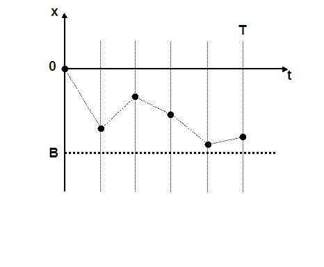
Figure 1: Example of path realization

When pricing barrier options with Monte Carlo simulations it is possible to miss some barrier hitting realization between two time steps. Consider the particular path realization of Figure 1. There are five time steps and none of the five underlying realizations have breached the barrier and therefore the path is going to count in the payoff sum. Following the idea presented in Shevchenko , we should weight the actualized payoff by a certain factor accounting for the probability of breaching the barrier between the discrete time points. As a weighting factor we can use the product over all time intervals $\Delta_{t}^{i}$ of the survival probability of the option,

$$w=\prod_{i=1}^{n}P_{surv}(\Delta_{t}^{i}).$$ (37)

Assuming that the volatility of the equity is constant over the interval $\Delta_{t}^{i}$, it is possible to derive an analytical expression for $P_{surv}(\Delta_{t}^{i})$ applicable in all different models treated in this paper. More precisely, under this assumption, $x(t+\Delta_{t}^{i})$ is normally distributed with mean $\mu_{x}$ and variance $\sigma^{2}_{x}$ given by

$$\mu_{x} = \frac{\rho_{Sr}\sigma_{r}\sigma_{S}}{\alpha}(1-e^{-\alpha\Delta_{t}^{i}}),$$

$$\sigma^{2}_{x} = \frac{\sigma^{2}_{r}}{2\alpha}(1-e^{-2\alpha\Delta_{t}^{i}}).$$ (38)

Using the well-known reflection principle (see Shreve ), we have the analytical expression for $P_{surv}(\Delta_{t}^{i})$

$$P_{surv}(\Delta_{t}^{i}) = P(x(s)>B,\ t<s\leq t+\Delta_{t}^{i})$$ (39)

$$= \mathcal{N}\left(\frac{-B+\mu_{x}\Delta_{t}^{i}}{\sigma_{x}\sqrt{\Delta_{t}^{i}}}\right)-e^{(\frac{-2B\mu_{x}}{\sigma^{2}_{x}})}\mathcal{N}\left(\frac{B+\mu_{x}\Delta_{t}^{i}}{\sigma_{x}\sqrt{\Delta_{t}^{i}}}\right).$$ (40)

The last assumption about the volatility of the equity is in contradiction with the nature of the LVHW and the SZHW models. However, as time intervals become smaller, this assumption is more and more justified.

The price of the “down-and-in GAO” can easily be computed from the price of the “down-and-out GAO” and the “pure GAO” by using the following relation

$$C^{DI}(x,0,T)=C(x,0,T)-C^{DO}(x,0,T).$$ (41)

Note that for knock-in type options, the survival probability is readily derived from the one coming from the corresponding knock-out type option by complementarity ($P_{surv}^{KI}=1-P_{surv}^{KO}$).

5 Numerical results

In this section we study the contribution of using a local volatility model with Hull and White stochastic interest rates (LVHW) (introduced in Section 2) to the pricing of Variable Annuity Guarantees. More precisely, we compare GAO, GMIB Rider and two barrier types GAO prices obtained by using the LVHW model to those obtained with the Schöbel-Zhu Hull-White (SZHW) stochastic volatility model and the Black-Scholes with Hull and White stochastic interest rates (BSHW). For a fair analysis, one first has to calibrate these three models to the same options market data. For this end, we have used the same data as in (van_Haastrecht_GAO, ). More precisely, the equity components (fund) of the Variable Annuity Guarantees considered are on one hand the EuroStoxx50 index (EU) and on the other hand the S&P500 index (US). In the following subsection we explain in details the calibration of the three models. We summarize the calibration of the interest rate parameters and the calibration of the SZHW and the BSHW made in (van_Haastrecht_GAO, ) and then we explain the calibration of the local volatility surface for the equity component in our LVHW model. In Subsection 5.3 we compare GAO values obtained by using the LVHW model with the SZHW and the BSHW prices studied in (van_Haastrecht_GAO, ). In Subsection 5.4 and Subsection 5.5, we do the same study for path-dependent Variable Annuity Guarantees namely GMIB Riders and barrier type GAOs.

5.1 Calibration to the Vanilla option’s Market

In order to compare LVHW GAO results to the ones obtained in the BSHW and the SZHW models presented in van Haastrecht et al. (van_Haastrecht_GAO, ) we are using Hull and White parameters and the implied volatility curve they have used. In (van_Haastrecht_GAO, ), interest rate parameters are calibrated to EU and US swaption markets using swaption mid prices of the 31st of July 2007. Moreover, the effective 10 years correlation between the log equity returns and the interest rates is determined by time series analysis of the 10-year swap rate and the log returns of the EuroStoxx50 index (EU) and the S&P500 index (US) over the period from February 2002 to July 2007 and turns out to be resp. $34.65\%$ and $14.64\%$ for the EU and the US market. The equity parameters in the SZHW and BSHW models are calibrated by using vanilla option prices on the EuroStoxx50 and S&P500 index obtained from the implied volatility service of MarkIT.

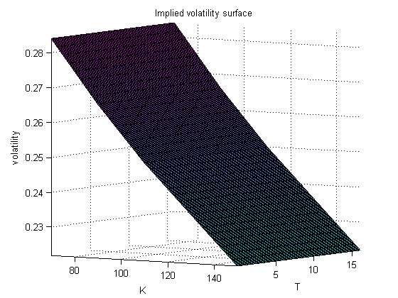
(a) implied volatility surface

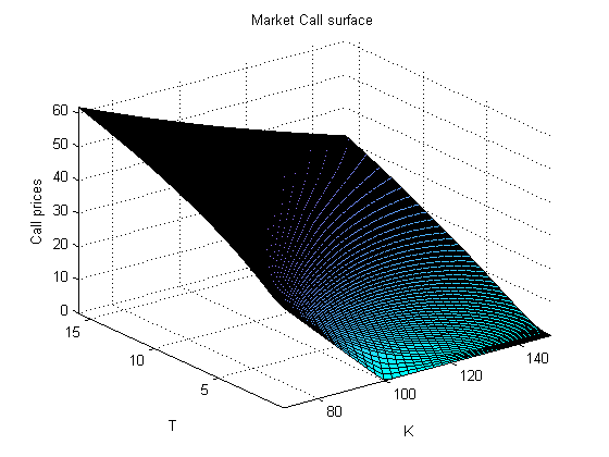
(b) market call prices

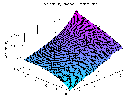
(c) local volatility (stochastic interest rates)

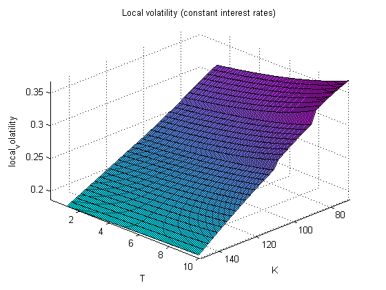
(d) local volatility (constant interest rates)

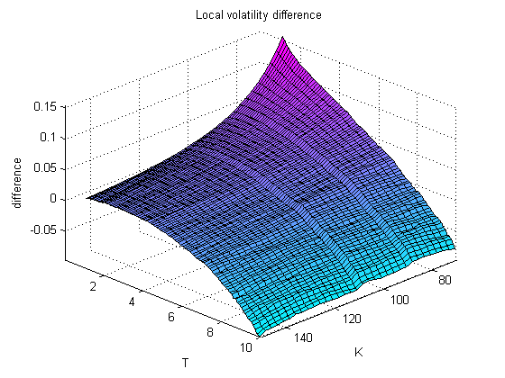
(e) difference

Figure 8: Plot of the implied volatility (built from the 10-years S&P500 implied volatility curve and assuming a constant volatility with respect to the maturity ($\frac{\partial\sigma_{imp}}{\partial T}=0.00$)), the corresponding market call prices surface, the associated local volatility obtained in both stochastic and constant interest rates framework and finally, the difference between these two local volatilities.

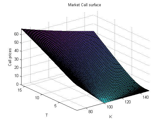
(b) market call prices

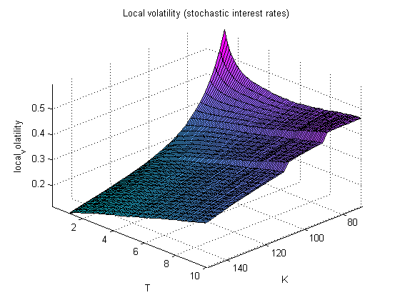
(c) local volatility (stochastic interest rates)

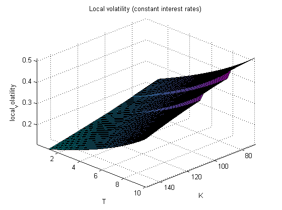
(d) local volatility (constant interest rates)

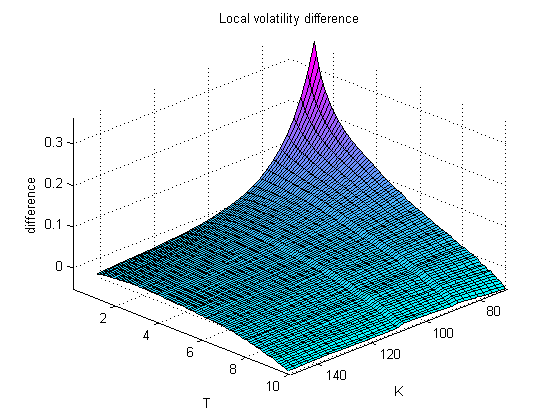
(e) difference

Figure 9: Plot of the implied volatility (built from the 10-years S&P500 implied volatility curve and assuming an increasing volatility with respect to the maturity ($\frac{\partial\sigma_{imp}}{\partial T}=0.01$)), the corresponding market call prices surface, the associated local volatility obtained in both stochastic and constant interest rates framework and finally, the difference between these two local volatilities.

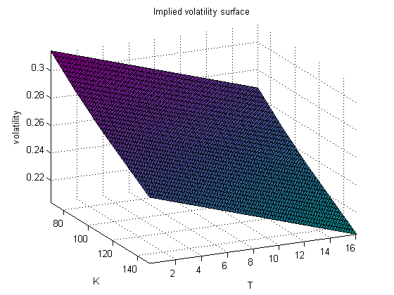
(a) implied volatility surface

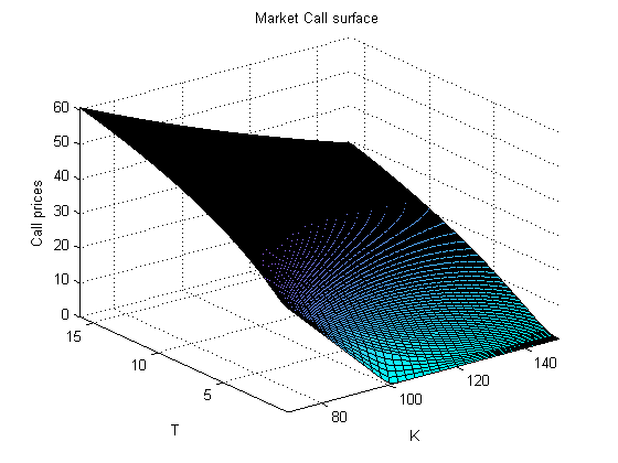
(b) market call prices

(c) local volatility (stochastic interest rates)

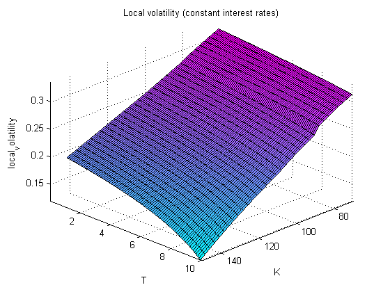
(d) local volatility (constant interest rates)

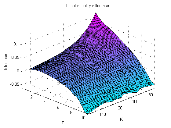
(e) difference

Figure 10: Plot of the implied volatility (built from the 10-years S&P500 implied volatility curve and assuming an decreasing volatility with respect to the maturity ($\frac{\partial\sigma_{imp}}{\partial T}=-0.003$)), the corresponding market call prices surface, the associated local volatility obtained in both stochastic and constant interest rates framework and finally, the difference between these two local volatilities.

In (van_Haastrecht_GAO, ) the authors have calibrated the equity model to market option prices maturing in 10 years time. In the LVHW model, the equity volatility is a local volatility surface and the calibration consists in building this surface using equation (LABEL:locvol_implied_C). This calibration procedure uses the whole implied volatility surface and returns a local volatility for all strikes and all maturities. In this paper we consider three different cases. In a first case, we assume that the implied volatility is constant with respect to the maturity ($\frac{\partial\sigma_{imp}}{\partial T}=0$) and in that case we denote the local volatility model by LVHW1. The second case denoted by LVHW2 considers an increasing term structure ($\frac{\partial\sigma_{imp}}{\partial T}=0.01$) and finally we consider the case LVHW3 where the implied volatility is a decreasing function of the maturity ($\frac{\partial\sigma_{imp}}{\partial T}=-0.003$). Note that for the aid of a fair comparison between the models, we have always kept the same volatility smile at time $T=10$. A plot of the three complete implied volatility surfaces and the resulting market call option prices can be found in Appendix C (see Figures 8(a), 8(b), 9(a), 9(b), 10(a), 10(b) for US data and 11(a), 11(b), 12(a), 12(b), 13(a), 13(b) for EUR data). Following the Monte Carlo approach given in Section 3.2, we have found the corresponding local volatility surface, see namely Figure 8(c), 9(c), 10(c) for the US data and 11(c), 12(c), 13(c) for the EUR data.

Implied volatility, 10-year call options, US
strike	Market	BSHW	SZHW	LVHW1 ($\pm$ 95% interval)
80	27.50%	25.80%	27.50%	27.503% ($\pm$ 0.01778 %)
90	26.60%	25.80%	26.60%	26.601% ($\pm$ 0.01745 %)
95	26.20%	25.80%	26.20%	26.198% ($\pm$ 0.01693 %)
100	25.80%	25.80%	25.80%	25.800% ($\pm$ 0.01631 %)
105	25.40%	25.80%	25.40%	25.397% ($\pm$ 0.01501 %)
110	25.00%	25.80%	25.00%	24.998% ($\pm$ 0.01432 %)
120	24.30%	25.80%	24.40%	24.333% ($\pm$ 0.01325 %)
Implied volatility, 10-year call options, EUR
strike	Market	BSHW	SZHW	LVHW1 ($\pm$ 95% interval)
80	27.80%	26.40%	27.90%	27.826% ($\pm$ 0.0214 %)
90	27.10%	26.40%	27.10%	27.103% ($\pm$ 0.0200 %)
95	26.70%	26.40%	26.70%	26.699% ($\pm$ 0.0194 %)
100	26.40%	26.40%	26.40%	26.396% ($\pm$ 0.0189 %)
105	26.00%	26.40%	26.00%	25.999% ($\pm$ 0.0181 %)
110	25.70%	26.40%	25.70%	25.702% ($\pm$ 0.0173 %)
120	25.10%	26.40%	25.10%	25.101% ($\pm$ 0.0165 %)

Table 1: Comparison of the implied volatility curve (for 10-year call options) generated by the SZHW, the BSHW and the LVHW1 models after being calibrated over the market implied volatility. US and European market implied volatilities as well as the BSHW and SZHW results are coming from van_Haastrecht_GAO .

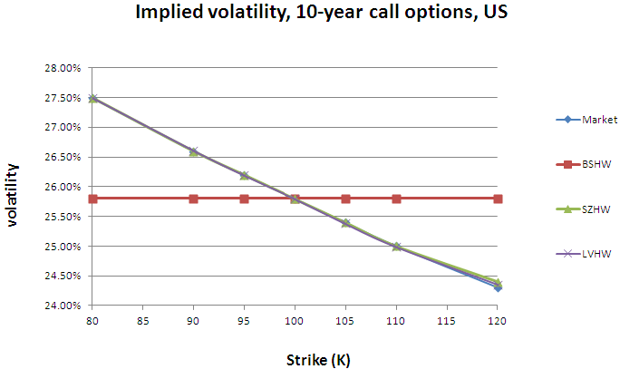
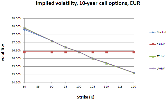
Figure 2: Comparison of the market implied volatility curve (for 10-year call options) and the three implied volatility curves coming from the SZHW, the BSHW and the LVHW1 models after calibration.

Stochastic volatility and local volatility models are both able to reproduce the market smile. For example, in Table 1, we compare the market implied volatility (for a range of seven different strikes and a fixed maturity $T=10$) with the calibrated volatility of each of the three models. The volatility curves of Table 1 generated by the market and these three models in the US and European 10 years maturity vanilla options market are presented in Figure 2. We notice that the local volatility model (LVHW) and the stochastic volatility model (SZHW) are both well calibrated since they are able to generate the Smile/Skew quite close to the market one. Note that, the LVHW1 implied volatilities are extracted from the European call values obtained by Monte Carlo simulations. Therefore, in the last column of Table 1, one also gives the corresponding $\pm$ 95% confidence interval. However, contrarily to the SZHW model, the LVHW model has to be calibrated over the whole implied volatility surface and as we will see in Subsection 5.3, 5.4 and 5.5, this fact has an impact to the price of Variable Annuity Guarantees.

5.2 A numerical comparison between local volatility with and without stochastic interest rates

In Section 3.3, equation (16) gives the difference between the tractable Dupire local volatility function $\sigma_{1f}(T,K)$ coming from the one-factor Gaussian model and the one which takes into account the effects of stochastic interest rates $\sigma_{2f}(T,K)$.

Note that the difference between $\sigma_{2f}(T,K)$ and $\sigma_{1f}(T,K)$ can be derived in terms of implied volatilities ($\sigma_{imp}$) by using equation (LABEL:locvol_implied_C) and (6) and leads to

$$\sigma_{2f}^{2}(T,K)-\sigma_{1f}^{2}(T,K)=\frac{Kr(0)e^{-r(0)T}\mathcal{N}(d_{-})-Vega^{BS}r(0)K\frac{\partial\sigma_{imp}}{\partial K}+KP(0,T)\mathbf{E}^{Q_{T}}[r(T)\textbf{1}_{\{S(T)>K\}}]}{\frac{1}{2}K^{2}Vega^{BS}(\frac{1}{\sigma_{imp}K^{2}T}+\frac{2d_{+}}{\sigma_{imp}K\sqrt{T}}\frac{\partial\sigma_{imp}}{\partial K}+\frac{\partial^{2}\sigma_{imp}}{\partial K^{2}}+\frac{d_{+}d_{-}}{\sigma_{imp}}(\frac{\partial\sigma_{imp}}{\partial K})^{2})}$$ (42)

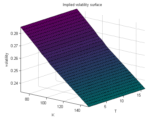
(a) implied volatility surface

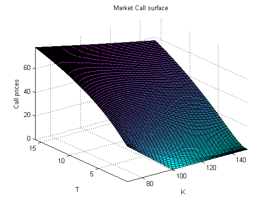
(b) market call prices

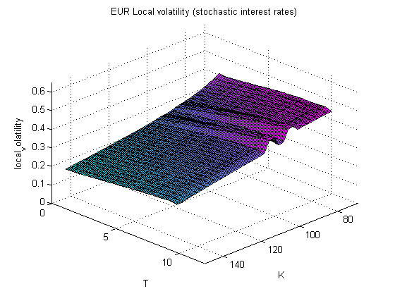
(c) local volatility (stochastic interest rates)

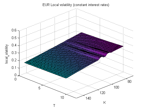
(d) local volatility (constant interest rates)

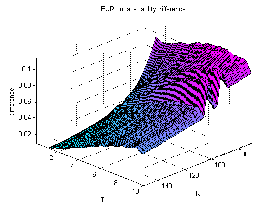
(e) difference

Figure 11: Plot of the implied volatility (built from the 10-years EuroStoxx50 implied volatility curve and assuming a constant volatility with respect to the maturity ($\frac{\partial\sigma_{imp}}{\partial T}=0.00$)), the corresponding market call prices surface, the associated local volatility obtained in both stochastic and constant interest rates framework and finally, the difference between these two local volatilities.

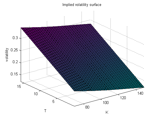
(a) implied volatility surface

(b) market call prices

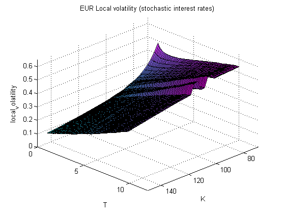
(c) local volatility (stochastic interest rates)

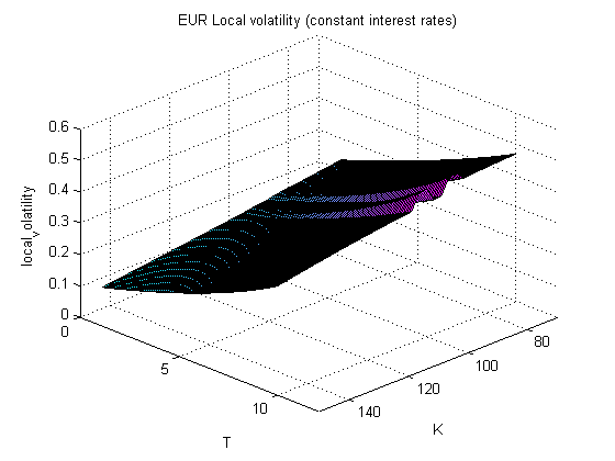
(d) local volatility (constant interest rates)

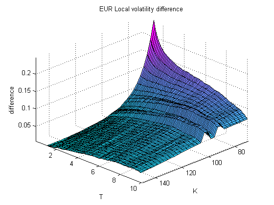
(e) difference

Figure 12: Plot of the implied volatility (built from the 10-years EuroStoxx50 implied volatility curve and assuming an increasing volatility with respect to the maturity ($\frac{\partial\sigma_{imp}}{\partial T}=0.01$)), the corresponding market call prices surface, the associated local volatility obtained in both stochastic and constant interest rates framework and finally, the difference between these two local volatilities.

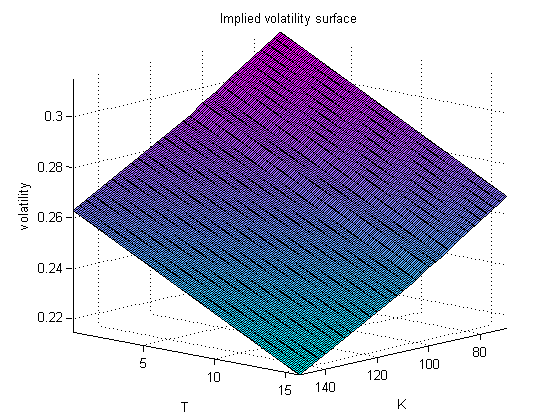
(a) implied volatility surface

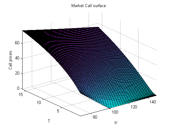
(b) market call prices

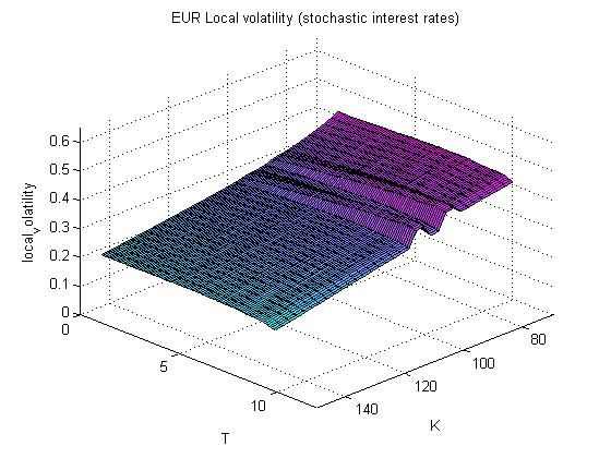
(c) local volatility (stochastic interest rates)

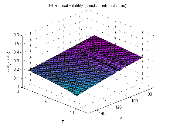
(d) local volatility (constant interest rates)

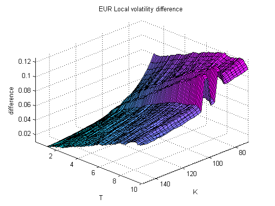
(e) difference

Figure 13: Plot of the implied volatility (built from the 10-years EuroStoxx50 implied volatility curve and assuming an decreasing volatility with respect to the maturity ($\frac{\partial\sigma_{imp}}{\partial T}=-0.003$)), the corresponding market call prices surface, the associated local volatility obtained in both stochastic and constant interest rates framework and finally, the difference between these two local volatilities.

In Figures 8(c), 9(c), 10(c), 8(d), 9(d), 10(d), 8(e), 9(e) and 10(e), we have plotted the local volatility coming from the stochastic interest rate framework ($\sigma_{2f}(T,K)$), the tractable Dupire local volatility ($\sigma_{1f}(T,K)$) and the surface generated by the difference between these two local volatilities in the US case and in Figures 11(c), 12(c), 13(c), 11(d), 12(d), 13(d), 11(e), 12(e) and 13(e), the analogues in the EUR case.

5.3 GAO results

In this section, we study the impact generated to GAO values by using the LVHW model with respect to prices given by using the BSHW and the SZHW models computed in (van_Haastrecht_GAO, ). We make therefore the same assumptions as in (van_Haastrecht_GAO, ), namely that the policyholder is 55 years old and that the retirement age is 65 (i.e. the maturity $T$ of the GAO option is 10 years). The fund value at time $0$, $S(0)$ is assumed to be 100. The survival rates are based on the PNMA00 table of the Continuous Mortality Investigation (CMI) for male pensioners.

In Table 2 we give prices obtained for the GAO using the LVHW model case 1 (LVHW1), the LVHW model case 2 (LVHW2), the LVHW model case 3 (LVHW3), the SZHW and the BSHW models for different guaranteed rates $g$. The results for the SZHW and BSHW models are obtained using the closed-form expression derived in resp. van_Haastrecht_GAO and Ballotta , which can be found in Appendix A for the convenience of the reader. Note that GAO prices presented in this section given by the BSHW and SZHW models are slightly different than those presented in van_Haastrecht_GAO . These differences come from the interpolation method we use for constructing the zero coupon bond curve. As it was pointed out in van_Haastrecht_GAO , GAO prices are sensitive to the interest rate curve and a small change in the zero coupon bond curve induces changes in GAO prices. The results for the LVHW model are obtained by using Monte Carlo simulations (100 000 simulations and 5000 steps). Table 3 and Figure 3 show the corrections induced by the LVHW and the SZHW models with respect to the BSHW model.

GAO Total Value US
$g$	BSHW	SZHW	LVHW1	SE	LVHW2	SE	LVHW3	SE
7%	00.906860	01.045977	01.021760	0.013730	00.970480	0.013374	01.059320	0.014154
8%	03.160037	03.567810	03.463430	0.026539	03.299570	0.025895	03.562870	0.027142
8.88%	07.101917	07.869198	07.584480	0.039751	07.332270	0.038987	07.808470	0.040443
9%	07.738402	08.555375	08.326130	0.041560	08.024770	0.040791	08.533410	0.042259
10%	14.880173	16.141393	15.690000	0.055644	15.271200	0.054907	16.034900	0.056342
11%	23.643769	25.267434	24.900900	0.066981	24.374900	0.066285	25.350600	0.067621
12%	33.689606	35.586279	35.117300	0.075737	34.507000	0.075030	35.626800	0.076333
13%	44.382228	46.570479	45.742500	0.082976	45.070200	0.082227	46.296100	0.083563
GAO Total Value EUR
$g$	BSHW	SZHW	LVHW1	SE	LVHW2	SE	LVHW3	SE
7%	00.395613	00.583057	00.486412	0.007961	00.428838	0.007326	00.502376	0.008006
8%	02.259404	02.882720	02.622240	0.019585	02.417440	0.018578	02.704880	0.019687
8.46%	04.095928	04.981611	04.664650	0.026196	04.323210	0.025098	04.719230	0.026313
9%	07.210501	08.393904	08.004080	0.033921	07.565690	0.032806	08.193780	0.034034
10%	15.421258	17.017295	16.597400	0.045658	15.974700	0.044657	16.880900	0.045707
11%	25.530806	27.369899	26.964500	0.053381	26.202900	0.052448	27.285900	0.053395
12%	36.282533	38.300598	37.885600	0.058946	37.031900	0.057988	38.234200	0.058954
13%	47.164918	49.351551	48.908600	0.063960	47.979600	0.062924	49.284400	0.063964

Table 2: Comparison of GAO total values in the BSHW, the SZHW and the LVHW1, LVHW2 and LVHW3 models for different guaranteed annuity rates $g$. The rates $g$ of $8.88\%$ and $8.46\%$ correspond to the at-the-money guaranteed annuity rates in the US and EUR market respectively.

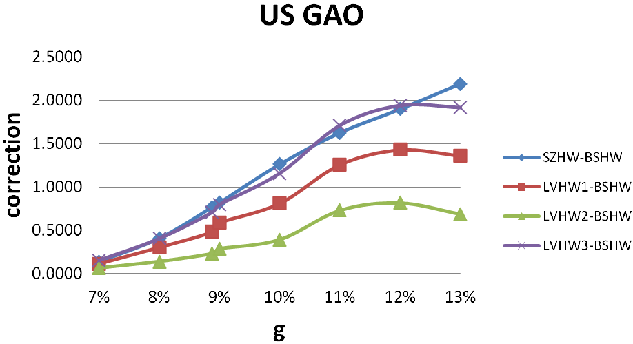
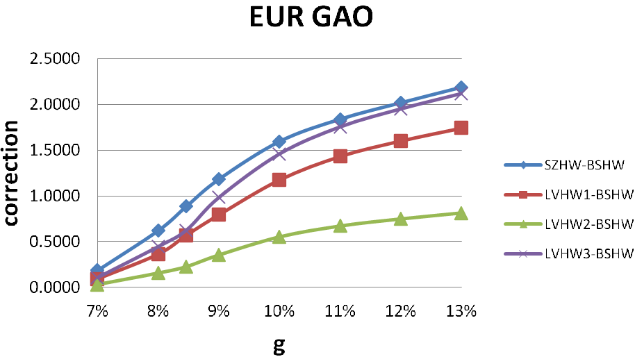
Figure 3: Graphical representation of the LVHW1, LVHW2, LVHW3 and the SZHW model corrections with respect to the BSHW model for different guaranteed annuity rates $g$.

US Correction
$g$	SZHW-BSHW	LVHW1-BSHW	LVHW2-BSHW	LVHW3-BSHW
7%	0.1391	0.1149	0.0636	0.1525
8%	0.4078	0.3034	0.1395	0.4028
8.88%	0.7673	0.4826	0.2304	0.7066
9%	0.8170	0.5877	0.2864	0.7950
10%	1.2612	0.8098	0.3910	1.1547
11%	1.6237	1.2571	0.7311	1.7068
12%	1.8967	1.4277	0.8174	1.9372
13%	2.1883	1.3603	0.6880	1.9139
EUR Correction
$g$	SZHW-BSHW	LVHW1-BSHW	LVHW2-BSHW	LVHW3-BSHW
7%	0.1874	0.0908	0.0332	0.1068
8%	0.6233	0.3628	0.1580	0.4455
8.46%	0.8857	0.5687	0.2273	0.6233
9%	1.1834	0.7936	0.3552	0.9833
10%	1.5960	1.1761	0.5534	1.4596
11%	1.8391	1.4337	0.6721	1.7551
12%	2.0181	1.6031	0.7494	1.9517
13%	2.1866	1.7437	0.8147	2.1195

Table 3: Corrections generated by the LVHW1, LVHW2, LVHW3 and the SZHW models with respect to the BSHW model for different guaranteed annuity rates $g$.

Table 4 presents the time value given by the difference between the GAO total value and its intrinsic value. The volatility of an option is an important factor for this time value since this value depends on the time until maturity and the volatility of the underlying instrument’s price. The time value reflects the probability that the option will gain in intrinsic value or become profitable to exercise before maturity. Figure 4 is a plot of the time value given by all considered models. For a deeper analysis about time value we refer the interested reader to van_Haastrecht_GAO .

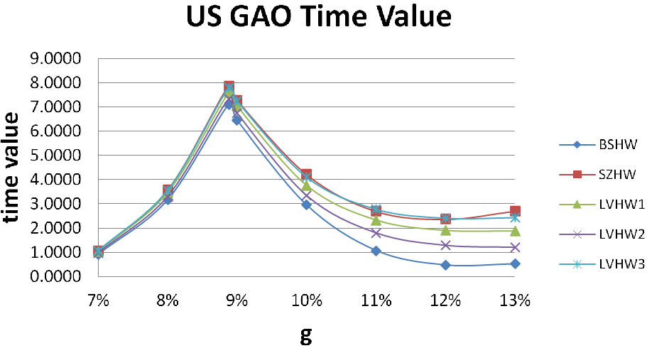
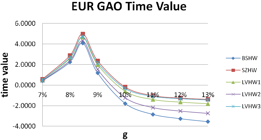
Figure 4: Graphical representation of GAO time values of the BSHW, the SZHW and the LVHW1, LVHW2 and LVHW3 models for different guaranteed annuity rates $g$.

GAO Time Value US
$g$	BSHW	SZHW	LVHW1	LVHW2	LVHW3
7%	0.9069	1.0460	1.0218	0.9705	1.0593
8%	3.1600	3.5678	3.4634	3.2996	3.5629
8.88%	7.1019	7.8692	7.5845	7.3323	7.8085
9%	6.4575	7.2745	7.0452	6.7439	7.2525
10%	2.9527	4.2140	3.7626	3.3438	4.1075
11%	1.0698	2.6935	2.3269	1.8009	2.7766
12%	0.4691	2.3658	1.8968	1.2865	2.4063
13%	0.5152	2.7034	1.8755	1.2032	2.4291
GAO Time Value EUR
$g$	BSHW	SZHW	LVHW1	LVHW2	LVHW3
7%	-0.3956	-0.5831	-0.4864	-0.4288	-0.5024
8%	-2.2594	-2.8827	-2.6222	-2.4174	-2.7049
8.46%	-4.0959	-4.9816	-4.6647	-4.3232	-4.7192
9%	-1.1839	-2.3673	-1.9775	-1.5391	-2.1672
10%	-1.7792	-0.1831	-0.6030	-1.2257	-0.3195
11%	-2.8435	-1.0044	-1.4098	-2.1714	-1.0884
12%	-3.2656	-1.2475	-1.6625	-2.5162	-1.3139
13%	-3.5570	-1.3704	-1.8134	-2.7424	-1.4376

Table 4: Comparison of GAO time values of the BSHW, the SZHW and the LVHW1, LVHW2 and LVHW3 models for different guaranteed annuity rates $g$.

These results show that the use of a non constant volatility model such as the SZHW model and the LVHW model has a significant impact on the total value and the time value of GAOs. Furthermore, the term structure of the implied volatility surface has also an influence on the total value. The numerical results show that the LVHW3 prices tend to the SZHW prices, whereas the LVHW2 prices are the lowest of the three LVHW models, but still above the BSHW prices. In the LVHW1 model prices remain between BSHW and SZHW values.

The fact that GAO prices obtained in different implied volatility scenarios turn out to be significantly different, underlines that it is most important to take always into account the whole implied volatility surface. This impact in GAO value can be justified by equation (30) where you can see the influence of the level of the equity spot $S_{t}$ in the dynamics of $x_{t}$ under the measure $Q_{S}$.

In van_Haastrecht_GAO , it is pointed out that GAO values are also particularly sensible to three different risk drivers namely the survival probabilities, the fund value and the interest rate market curve. From equation (32), we can easily deduce that an increase of $x\%$ of the equity fund value $S(0)$ will induce an $x\%$ increase of the GAO value. It is also clear that a shift in the mortality table will induce a shift in the GAO value in the same direction. Finally, a shift down applied to the interest rates curve will increase the GAO value. The sensibility of GAO prices with respect to the implied volatility, the survival probabilities, the fund value and the interest rates market curve underline the fact that for all practical purposes, the market data used can be as important as the model used.

5.4 GMIB Rider

In this section, we analyze how the BSHW, the SZHW and the LVHW models behave in the pricing of a GMIB Rider. This product has a strong dependence on the path of the equity fund $S$ coming from the anniversary component in the payoff, namely $\underset{n\in A}{max}(S(n))g\ddot{a}_{x}(T)$ (see equation (34)), where $A$ is the set of anniversary dates $A=\{1,2,...,T\}$. We use exactly the same initial data as for the GAO. More precisely, the policyholder is assumed to be 55 years old with a retirement age of 65 (i.e. the maturity $T$ of the GMIB Rider is 10 years). The fund value at time $0$, $S(0)$ is assumed to be 100. The survival rates are based on the PNMA00 table of the Continuous Mortality Investigation (CMI) for male pensioners. We present numerical results obtained in the US market only because European market leads to similar behavior in pricing and conclusions. The parameters used in each model are those obtained after calibration as explained in Section 3. In Table 5, we compare the price of a GMIB Rider for eight different guaranteed annuity rates $g$ and three different guaranteed annual rates $r_{g}$ (computed by using Monte Carlo simulations with 100000 simulations and 5000 steps). Note that currently, the standard rate $r_{g}$ offered by insurance companies is around $5\%$ (see GMIB ).

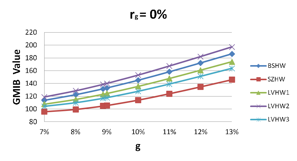
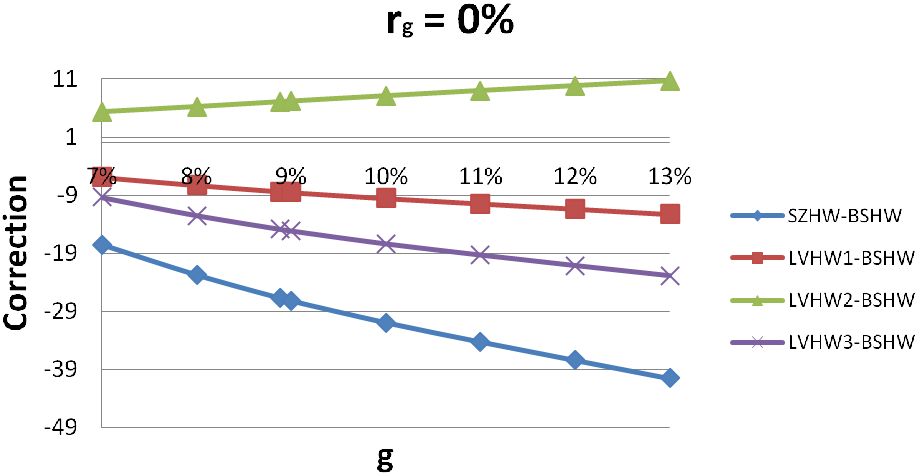
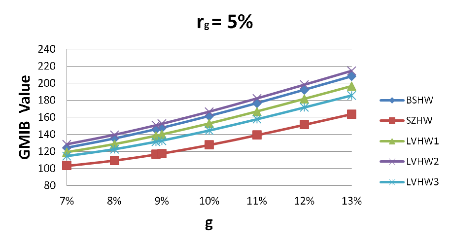
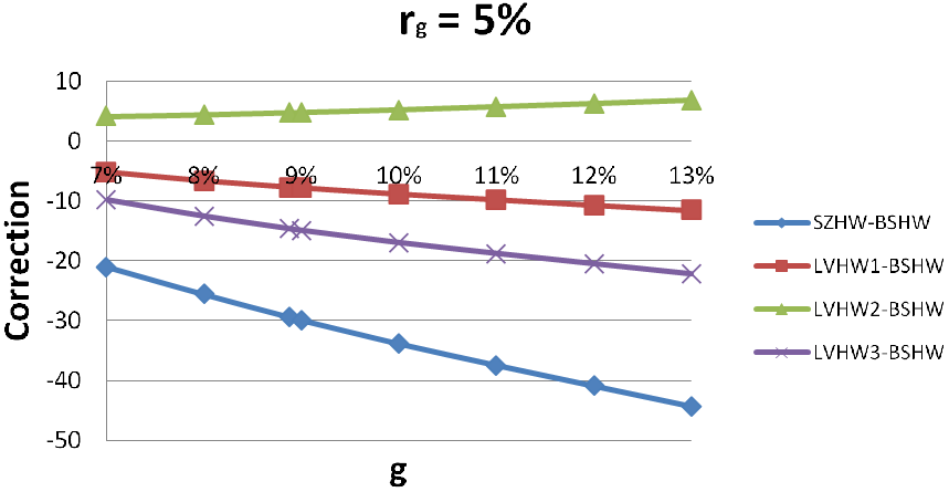
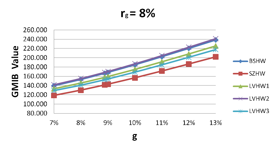
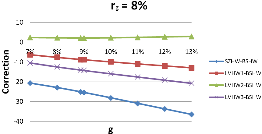
Figure 5: Graphical representation of GMIB Rider total values given by the SZHW, the LVHW1, LVHW2 and LVHW3 models for different guaranteed annuity rates $g$ and for different guaranteed annual rates $r_{g}$. The corrections given by each model with respect to the BSHW model are also presented.

Contrarily to the results obtained for GAOs (in Section 5.3), the corrections given to GMIB values by the SZHW model with respect to the BSHW ones are always negative. For GMIB Riders the highest values are always given by the LVHW2 model while the smallest values are coming from the SZHW model. In the GAO case, the SZHW and the LVHW3 GAO values where quite close and leading to the highest values among the observed models. For GMIB Riders, however, the smallest prices are given by the SZHW and the LVHW3 models, as illustrated in Figure 5.

US GMIB Rider Total Value $r_{g}=0\%$
$g$	BSHW	SE	SZHW	SE	LVHW1	SE	LVHW2	SE	LVHW3	SE
7%	113.5440	0.2892	095.9552	0.0720	107.6490	0.1235	118.8630	0.1497	104.1640	0.1185
8%	122.3090	0.2951	099.5474	0.0776	115.0510	0.1298	128.5280	0.1577	109.8140	0.1233
8.88%	131.4990	0.3063	104.7690	0.0810	123.1420	0.1375	138.5730	0.1675	116.6260	0.1300
9%	132.8540	0.3083	105.6330	0.0896	124.3560	0.1387	140.0450	0.1690	117.6870	0.1310
10%	144.9830	0.3290	114.0400	0.0900	135.4570	0.1503	153.1060	0.1830	127.5870	0.1414
11%	158.2590	0.3557	124.0140	0.0938	147.8150	0.1636	167.3030	0.1990	138.9400	0.1536
12%	172.1850	0.3857	134.7800	0.1001	160.8320	0.1779	182.0900	0.2163	151.0450	0.1669
13%	186.3910	0.4171	145.8680	0.1077	174.1050	0.1925	197.1540	0.2341	163.4870	0.1806
US GMIB Rider Total Value $r_{g}=5\%$
$g$	BSHW	SE	SZHW	SE	LVHW1	SE	LVHW2	SE	LVHW3	SE
7%	124.253	0.2770	103.267	0.0713	119.021	0.1325	128.412	0.1577	114.516	0.1238
8%	135.096	0.2804	109.527	0.0738	128.454	0.1404	139.552	0.1666	122.620	0.1308
8.88%	145.994	0.2897	116.600	0.0768	138.313	0.1495	150.778	0.1767	131.384	0.1392
9%	147.576	0.2914	117.684	0.0818	139.766	0.1509	152.407	0.1783	132.699	0.1405
10%	161.528	0.3105	127.717	0.0830	152.701	0.1637	166.769	0.1927	144.587	0.1526
11%	176.537	0.3354	139.129	0.0859	166.782	0.1783	182.269	0.2093	157.761	0.1663
12%	192.154	0.3637	151.289	0.0877	181.503	0.1938	198.384	0.2272	171.643	0.1809
13%	208.030	0.3934	163.754	0.0944	196.494	0.2097	214.782	0.2459	185.806	0.1959
US GMIB Rider Total Value $r_{g}=8\%$
$g$	BSHW	SE	SZHW	SE	LVHW1	SE	LVHW2	SE	LVHW3	SE
7%	139.3960	0.2579	118.7200	0.0759	133.1170	0.1441	141.7610	0.1600	128.9560	0.1339
8%	153.0990	0.2589	130.1780	0.0775	145.4630	0.1542	155.3320	0.1710	140.6420	0.1439
8.88%	166.4050	0.2661	141.3230	0.0820	157.6800	0.1651	168.5760	0.1831	152.3680	0.1547
9%	168.3040	0.2676	142.9100	0.0828	159.4420	0.1667	170.4710	0.1849	154.0570	0.1563
10%	184.7890	0.2834	156.6750	0.0904	174.8370	0.1812	187.0320	0.2013	168.8660	0.1705
11%	202.2100	0.3051	171.2920	0.0988	191.2250	0.1972	204.6760	0.2197	184.6850	0.1863
12%	220.1720	0.3304	186.4520	0.1075	208.1920	0.2141	222.8780	0.2389	201.0500	0.2027
13%	238.3830	0.3571	201.8650	0.1163	225.4030	0.2314	241.3100	0.2586	217.6730	0.2194

Table 5: Comparison of GMIB Rider total values of the BSHW, the SZHW and the LVHW1, LVHW2 and LVHW3 models for different guaranteed annuity rates $g$ and guaranteed annual rates $r_{g}$ of $0\%$, $5\%$ and of $8\%$.

5.5 Barrier GAOs

In this subsection, we compare the LVHW price, the SZHW price and the price obtained by using the three different cases of the LVHW model for “down-and-out GAOs” and “down-and-in GAOs” given by equation (36) and (41) respectively and computed by using Monte Carlo simulations (100 000 simulations and 5000 steps). While GMIB Riders are path-dependent especially in $S(t)$, these barrier options are particularly dependent on the path of the interest rates $r(t)$. In Table 6, 7, 8, 9 and 10, total values of “down-and-out GAOs” with five different barriers are presented. The first barrier is taken to be equal to $B=-0.015$ and corresponds to a market annuity rate $r_{x}(T)$ equal to 8%. More precisely, when $x^{*}=-0.015$ and $r_{x}(T)=8\%$, the definition of market annuity rate holds, namely,

$$\overset{\omega-(x+T)}{\underset{n=0}{\sum}}\phantom{.}_{n}p_{x+T}A(T,T+n)e^{-b(T,T+n)x^{*}}=1/r_{x}(T).$$

The other barriers correspond to rates $r_{x}(T)$ of 7%, 6%, 5% and 4% respectively or equivalently to barrier levels $B$ equal to -0.033, -0.05225, -0.0791 and -0.1019 respectively. Note that since the initial value of $x(0)$ is equal to 0, the barrier level $B$ has to be smaller and consequently strictly negative. The value of a “pure GAO” is given in the last column of Table 6, 7, 8, 9 and 10. When the barrier level is equal to 4%, the “down-and-out GAO” value is close to the GAO value. In that case, the survival probability of the “down-and-out GAO” is close to one. A graphical representation of the corrections given by each model with respect to the BSHW model can be found in Figure 6, and this for eight different guaranteed annuity rates $g$.

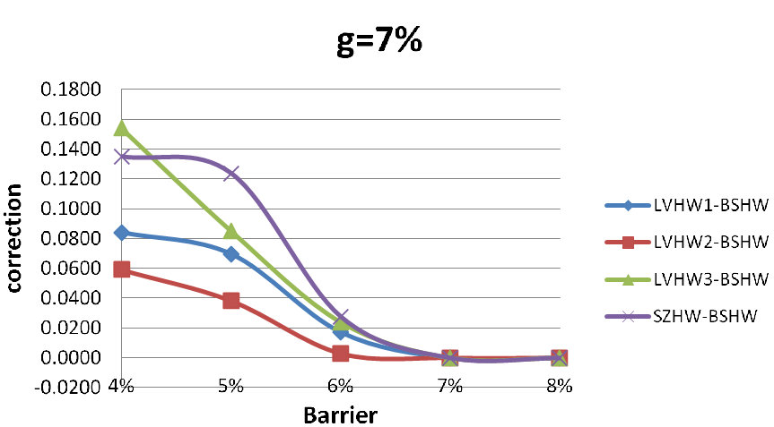
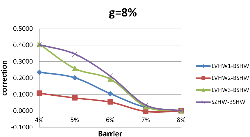
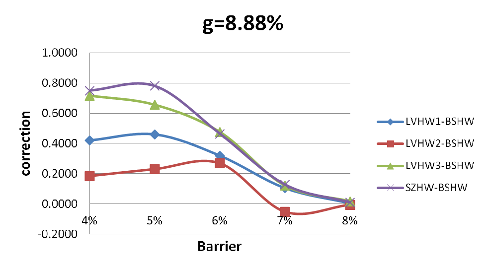
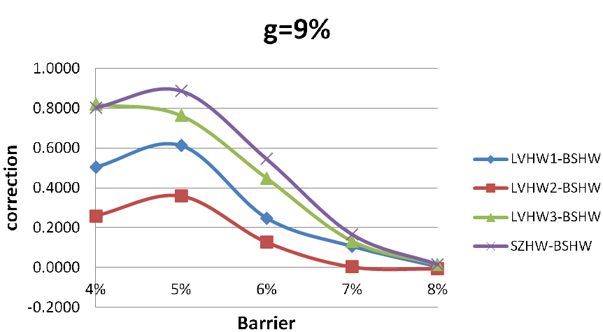
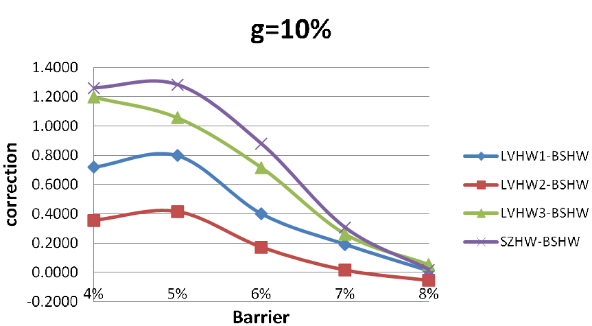
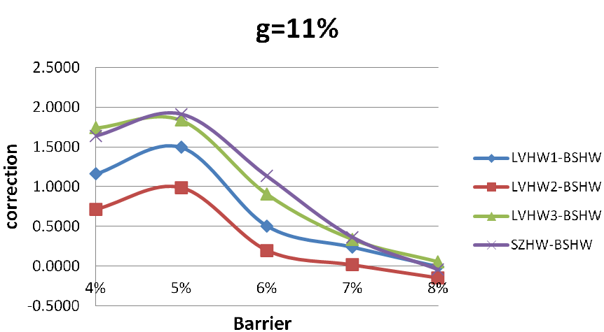
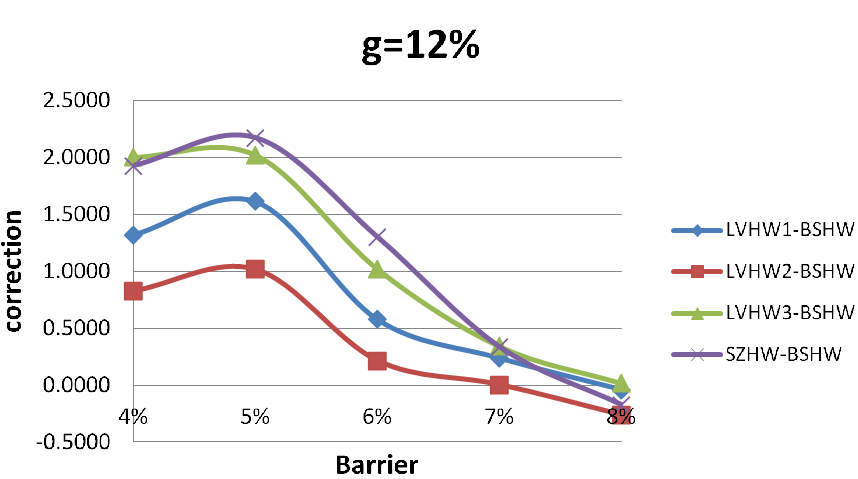
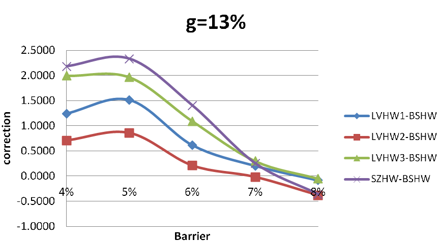
Figure 6: Graphical representation of DO GAO corrections of the SZHW, the LVHW1, LVHW2 and LVHW3 models for different guaranteed annuity rates $g$ with respect to the BSHW model.

BSHW DO GAO Total Value (US)						BSHW GAO
	8.00%	7.00%	6.00%	5.00%	4.00%
7%	00.0000	00.0000	00.2314	00.8138	00.9046	00.9069
(SE)	0(0.0000)	0(0.0000)	0(0.0041)	0(0.0112)	0(0.0131)
8%	00.0000	00.3411	01.7787	03.0548	03.1415	03.1600
(SE)	0(0.0000)	0(0.0047)	0(0.0150)	0(0.0238)	0(0.0256)
8.88%	00.1607	02.0274	05.0804	06.8923	07.0821	07.1019
(SE)	0(0.0028)	0(0.0144)	0(0.0275)	0(0.0369)	0(0.0387)
9%	00.2273	02.3625	05.6478	07.6506	07.7299	07.7384
(SE)	0(0.0036)	0(0.0159)	0(0.0293)	0(0.0387)	0(0.0405)
10%	01.5112	06.6738	12.0277	14.7523	14.8721	14.8802
(SE)	0(0.0125)	0(0.0296)	0(0.0435)	0(0.0529)	0(0.0546)
11%	04.0316	12.8157	20.2984	23.0443	23.5709	23.6438
(SE)	0(0.0240)	0(0.0429)	0(0.0554)	0(0.0643)	0(0.0661)
12%	07.3759	20.0008	29.6144	33.0740	33.6186	33.6896
(SE)	0(0.0365)	0(0.0553)	0(0.0650)	0(0.0731)	0(0.0749)
13%	11.0977	27.6196	39.3708	44.2385	44.3125	44.3822
(SE)	0(0.0497)	0(0.0673)	0(0.0733)	0(0.0803)	0(0.0821)

Table 6: “Down-and-out GAO” total values given by the BSHW model for eight different guaranteed annuity rates $g$ and for five different barriers. The pure GAO values for the eight different guaranteed annuity rates $g$ are also given in the last column.

SZHW DO GAO Total Value (US)						SZHW GAO
	8.00%	7.00%	6.00%	5.00%	4.00%
7.00%	00.0000	00.0000	00.2591	00.9375	01.0345	01.0460
(SE)	0(0.0000)	0(0.0000)	0(0.0043)	0(0.0122)	0(0.0141)
8.00%	00.0000	00.3753	01.9895	03.3998	03.5433	03.5678
(SE)	0(0.0000)	0(0.0049)	0(0.0156)	0(0.0253)	0(0.0272)
8.88%	00.1704	02.1545	05.5442	07.6723	07.8320	07.8692
(SE)	0(0.0029)	0(0.0149)	0(0.0285)	0(0.0387)	0(0.0405)
9.00%	00.2413	02.5278	06.1930	08.3709	08.5336	08.5554
(SE)	0(0.0037)	0(0.0165)	0(0.0303)	0(0.0405)	0(0.0423)
10.00%	01.5298	06.9793	12.9071	15.8655	16.0528	16.1414
(SE)	0(0.0127)	0(0.0303)	0(0.0445)	0(0.0546)	0(0.0563)
11.00%	03.9929	13.1818	21.4323	25.1681	25.1995	25.2674
(SE)	0(0.0242)	0(0.0437)	0(0.0562)	0(0.0657)	0(0.0675)
12.00%	07.2008	20.3345	30.9134	35.4296	35.5052	35.5863
(SE)	0(0.0368)	0(0.0564)	0(0.0658)	0(0.0743)	0(0.0761)
13.00%	10.7340	27.8709	40.7734	46.0700	46.3932	46.5705
(SE)	0(0.0500)	0(0.0689)	0(0.0742)	0(0.0815)	0(0.0833)

Table 7: “Down-and-out GAO” total values given by the SZHW model for eight different guaranteed annuity rates $g$ and for five different barriers. The pure GAO values for the eight different guaranteed annuity rates $g$ are also given in the last column.

LVHW1 DO GAO Total Value (US)						LVHW1 GAO
	8.00%	7.00%	6.00%	5.00%	4.00%
7%	00.0000	00.0000	00.2486	00.8834	00.9887	01.0218
(SE)	0(0.0000)	0(0.0000)	0(0.0079)	0(0.0133)	0(0.0141)	0(0.0137)
8%	00.0000	00.3626	01.8830	03.2555	03.3862	03.4634
(SE)	0(0.0000)	0(0.0102)	0(0.0197)	0(0.0262)	0(0.0270)	0(0.0265)
8.88%	00.1666	02.1331	05.4004	07.3525	07.5028	07.5845
(SE)	0(0.0085)	0(0.0213)	0(0.0327)	0(0.0395)	0(0.0403)	0(0.0398)
9%	00.2311	02.4683	05.8958	08.0631	08.2038	08.3261
(SE)	0(0.0096)	0(0.0230)	0(0.0345)	0(0.0414)	0(0.0421)	0(0.0416)
10%	01.5206	06.8641	12.4280	15.3804	15.5415	15.6900
(SE)	0(0.0208)	0(0.0370)	0(0.0487)	0(0.0556)	0(0.0562)	0(0.0556)
11%	04.0272	13.0565	20.8054	24.5382	24.7208	24.9009
(SE)	0(0.0336)	0(0.0499)	0(0.0604)	0(0.0671)	0(0.0677)	0(0.0670)
12%	07.3354	20.2375	30.1895	34.6890	34.8983	35.1173
(SE)	0(0.0470)	0(0.0615)	0(0.0696)	0(0.0759)	0(0.0765)	0(0.0757)
13%	11.0113	27.8210	39.9830	45.2484	45.4933	45.7425
(SE)	0(0.0608)	0(0.0724)	0(0.0775)	0(0.0833)	0(0.0839)	0(0.0830)

Table 8: “Down-and-out GAO” total values given by the LVHW1 model for eight different guaranteed annuity rates $g$ and for five different barriers. In the last column, one has the pure GAO values for the eight different guaranteed annuity rates $g$.

LVHW2 DO GAO Total Value (US)						LVHW2 GAO
	8.00%	7.00%	6.00%	5.00%	4.00%
7%	00.0000	00.0000	00.2343	00.8521	00.9537	00.9705
(SE)	0(0.0000)	0(0.0000)	0(0.0077)	0(0.0131)	0(0.0139)	0(0.0134)
8%	00.0000	00.3384	01.8329	03.1339	03.2095	03.2996
(SE)	0(0.0000)	0(0.0101)	0(0.0195)	0(0.0259)	0(0.0267)	0(0.0259)
8.88%	00.1554	01.9745	05.3501	07.1236	07.2671	07.3323
(SE)	0(0.0081)	0(0.0211)	0(0.0324)	0(0.0392)	0(0.0400)	0(0.0390)
9%	00.2206	02.3656	05.7748	07.8091	07.9390	08.0248
(SE)	0(0.0092)	0(0.0228)	0(0.0342)	0(0.0410)	0(0.0418)	0(0.0408)
10%	01.4562	06.6893	12.2000	14.9976	15.1776	15.2712
(SE)	0(0.0203)	0(0.0368)	0(0.0484)	0(0.0552)	0(0.0560)	0(0.0549)
11%	03.8866	12.8339	20.4983	24.0320	24.2953	24.3749
(SE)	0(0.0331)	0(0.0497)	0(0.0602)	0(0.0667)	0(0.0675)	0(0.0663)
12%	07.1146	20.0048	29.8277	34.0920	34.4322	34.5070
(SE)	0(0.0465)	0(0.0613)	0(0.0695)	0(0.0756)	0(0.0763)	0(0.0750)
13%	10.7150	27.5991	39.5786	44.5937	44.9869	45.0702
(SE)	0(0.0602)	0(0.0723)	0(0.0774)	0(0.0829)	0(0.0837)	0(0.0822)

Table 9: “Down-and-out GAO” total values given by the LVHW2 model for eight different guaranteed annuity rates $g$ and for five different barriers. In the last column, one has the pure GAO values for the eight different guaranteed annuity rates $g$.

LVHW3 DO GAO Total Value (US)						LVHW3 GAO
	8.00%	7.00%	6.00%	5.00%	4.00%
7%	00.0000	00.0000	00.2554	00.8988	01.0565	01.0593
(SE)	0(0.0000)	0(0.0000)	0(0.0081)	0(0.0136)	0(0.0144)	0(0.0142)
8%	00.0000	00.3665	01.9723	03.3129	03.5442	03.5629
(SE)	0(0.0000)	0(0.0105)	0(0.0201)	0(0.0266)	0(0.0274)	0(0.0271)
8.88%	00.1784	02.1492	05.5560	07.5477	07.7981	07.8085
(SE)	0(0.0086)	0(0.0216)	0(0.0332)	0(0.0399)	0(0.0407)	0(0.0404)
9%	00.2411	02.4941	06.0965	08.2142	08.5003	08.5334
(SE)	0(0.0098)	0(0.0233)	0(0.0350)	0(0.0417)	0(0.0425)	0(0.0423)
10%	01.5628	06.9347	12.7441	15.6396	16.0209	16.0349
(SE)	0(0.0210)	0(0.0373)	0(0.0492)	0(0.0559)	0(0.0567)	0(0.0563)
11%	04.0876	13.1534	21.2053	24.8806	25.3019	25.3506
(SE)	0(0.0340)	0(0.0502)	0(0.0609)	0(0.0674)	0(0.0682)	0(0.0676)
12%	7.3917	20.3405	30.6314	35.0938	35.5751	35.6268
(SE)	0(0.0474)	0(0.0617)	0(0.0701)	0(0.0763)	0(0.0771)	0(0.0763)
13%	11.0452	27.9176	40.4625	45.7019	46.2445	46.2961
(SE)	0(0.0612)	0(0.0727)	0(0.0780)	0(0.0837)	0(0.0845)	0(0.0836)

Table 10: “Down-and-out GAO” total values given by the LVHW3 model for eight different guaranteed annuity rates $g$ and for five different barriers. In the last column, one has the pure GAO values for the eight different guaranteed annuity rates $g$.

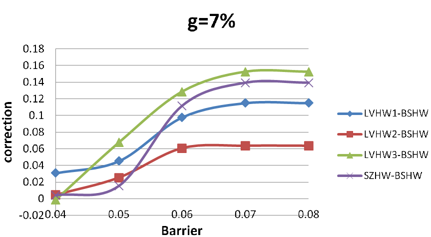
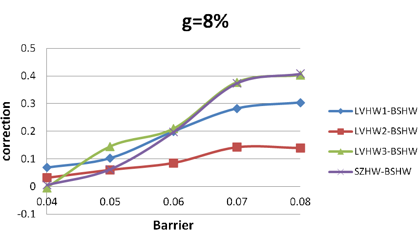
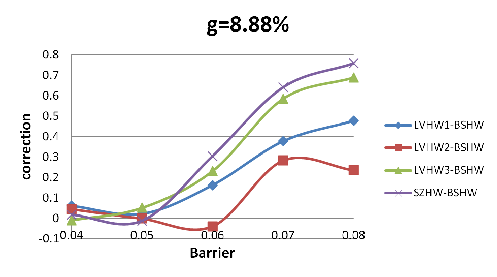
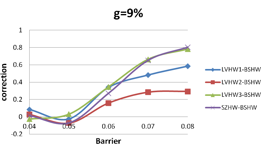
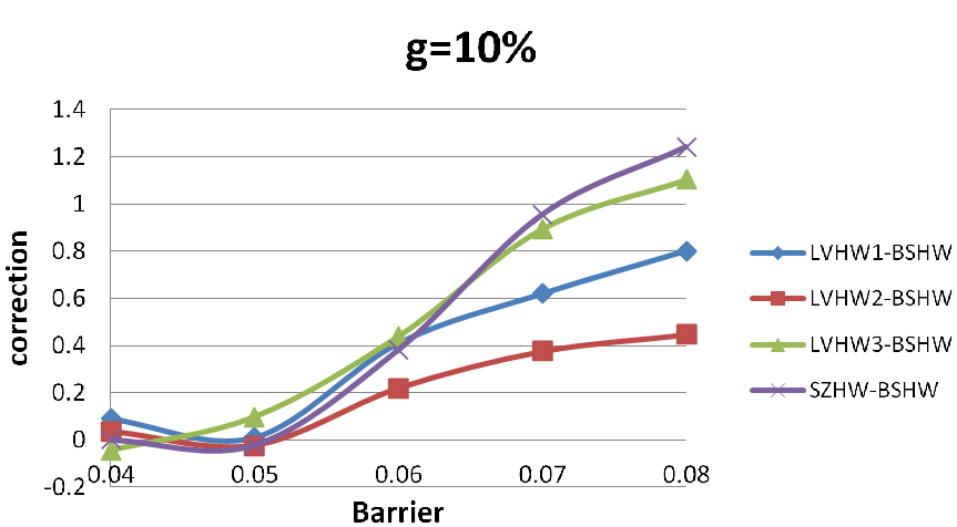
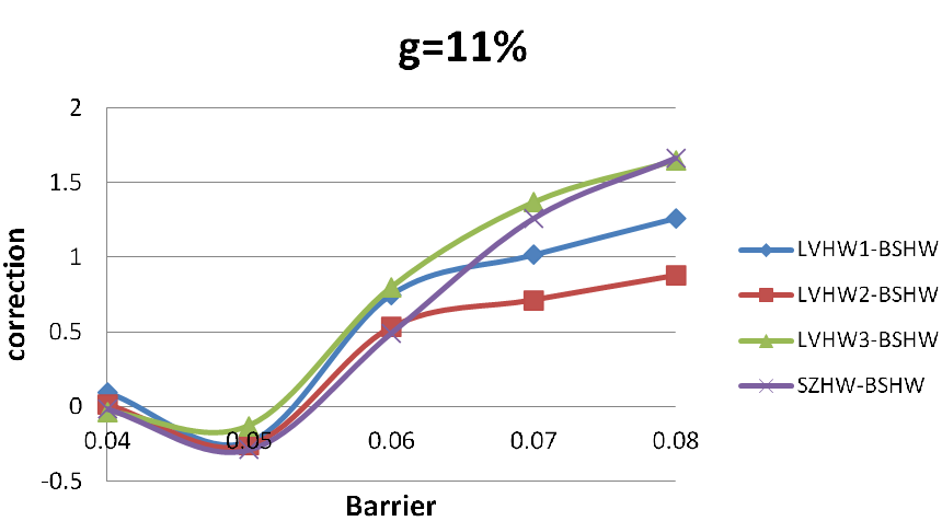
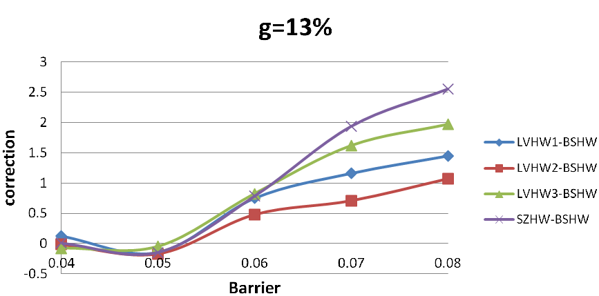
Figure 7: Graphical representation of DI GAO corrections of the SZHW, the LVHW1, LVHW2 and LVHW3 models for different guaranteed annuity rates $g$ with respect to the BSHW model.

The price of the “down-and-in GAO” can easily be computed from the price of the “down-and-out GAO” and the “pure GAO” by using the relation given by equation (41). In Appendix B, Table 11, total values of US “down-and-in GAOs” for the eight different guaranteed annuity rates $g$ and for the five different barriers are presented. Figure 7 in Appendix B illustrates the corrections for “down-and-in GAOs” given by each model with respect to the BSHW model for eight different guaranteed annuity rates $g$.

In the case of barrier GAOs the corrections given by each model are more complicated to analyze in the sense that there is no general conclusion with respect to the correction behavior. More precisely, we are not able to answer the question which model gives the highest values or the smallest ones because it depends on both the barrier level and of the guaranteed annuity rate $g$.

6 Conclusion

The local volatility model with stochastic interest rates is a suitable model to price and hedge long maturities life insurance contracts. This model takes into account the stochastic behavior of the interest rates as well as the vanilla market smile effects. The local volatility captures the whole implied volatility surface and is a deterministic function presenting an advantage for hedging strategies in comparison with stochastic volatility models for which the market is incomplete.

A first contribution of the paper is the calibration of a local volatility surface in a stochastic interest rates framework. We have developed a Monte Carlo approach for the calibration and this method has successfully been tested on US and European market call data.

The second contribution is the analysis of the impact of using a local volatility model to the price of long-dated insurance products as Variable Annuity Guarantees. More precisely, we have compared prices of GAO, GMIB Rider and barrier GAO obtained by using the local volatility model with stochastic interest rates to the prices given by a constant volatility and a stochastic volatility model all calibrated to the same data. The particularity of the GMIB Rider is the strong dependence on the path of the equity fund; whereas, the interest rate barrier type options have a strong dependence on the path of interest rates. The results confirm that calibrating such models to the vanilla market is by no means a guarantee that derivatives will be priced identically.

Where van_Haastrecht_GAO already pointed out that using a non constant volatility has a significant impact on the price of GAO we generalized this conclusion to GMIB Rider and Barrier GAOs and used local volatility models. Furthermore, we confirm that when using market data given in van_Haastrecht_GAO , the constant volatility Black Scholes model with stochastic interest rates turns out to underestimate the value of GAO compared to the Schöbel and Zhu stochastic volatility model with stochastic interest rates. However, we show that in a local volatility framework with stochastic interest rates, the price of GAO depends on the whole option’s implied volatility surface. Moreover, for GMIB Riders, the conclusion is the opposite, the SZHW model prices are always smaller than the corresponding BSHW model prices.

This paper underlines the fact that due to the sensibilities of Variable Annuity Guarantee prices with respect to the model used (after calibration to the Vanilla market), and also the sensibilities with respect to data, namely, the survival probability table and the yield curve, practitioners should be careful in their model choice as well as the market data chosen and the calibration of the model.

The results presented in this paper show that stochastic and local volatility models, perfectly calibrated on the same market implied volatility surface, do not imply the same prices for Variable Annuity Guarantees. In lipton3 , the authors underline that the market dynamics could be better approximated by a hybrid volatility model that contains both stochastic volatility dynamics and local volatility ones. The study of a pure local volatility model is crucial for the calibration of such hybrid volatility models (see (Deelstra-Rayee, )). For future research we plan to calibrate hybrid volatility models, based on the results obtained for the pure local volatility model. We further will study the impact of the hybrid volatility models to GAOs, GMIB Riders and barrier GAOs. The hedging performance of all these models is also left for future work.

Appendix A Explicit formula for the GAO price in the BSHW and SZHW models

In this appendix, we recall the explicit formula for a GAO price in the BSHW and in the SZHW models derived in Ballotta and van_Haastrecht_GAO respectively.

In the SZHW model, the fund value $S$, the interest rate $r$ and the volatility are governed by the following dynamics:

$$dS(t) = (r(t)-q)S(t)dt+\nu(t)S(t)dW^{Q}_{S}(t),$$

$$dr(t) = (\theta(t)-\alpha r(t))dt+\sigma_{r}dW^{Q}_{r}(t),$$

$$d\nu(t) = \kappa(\psi-\nu(t))dt+\tau dW^{Q}_{\nu}(t).$$

The dynamics of the fund $S(t)$, the interest rates $r(t)$ and the volatility of the fund $\nu(t)$ are linked by the following correlation structure:

$$E^{Q}[dW^{Q}_{S}dW^{Q}_{r}]=\rho_{Sr}dt,$$

$$E^{Q}[dW^{Q}_{S}dW^{Q}_{\nu}]=\rho_{S\nu}dt,$$

$$E^{Q}[dW^{Q}_{\nu}dW^{Q}_{r}]=\rho_{\nu r}dt.$$

The explicit formula of the GAO price is given by

$$C(x,0,T)=\phantom{.}_{T}p_{x}gS(0)\sum_{n=0}^{\omega-(x+T)}\phantom{.}{}_{n}p_{x+T}(F_{n}\mathcal{N}(d_{1}^{n})-K_{n}\mathcal{N}(d_{2}^{n})),$$ (43)

where the strikes are given by $K_{n}=A(T,T+n)e^{-b(T,T+n)x^{*}}$ with $x^{*}$ solving

$$\overset{\omega-(x+T)}{\underset{i=0}{\sum}}\phantom{.}_{n}p_{x+T}A(T,T+n)e^{-b(T,T+n)x^{*}}=1/g$$

with

$$F_{n} = e^{M_{n}+\frac{1}{2}V_{n}}$$

$$d_{1}^{n} = \frac{\ln(F_{n}/K_{n})+\frac{1}{2}V_{n}}{\sqrt{V_{n}}}$$

$$d_{2}^{n} = d_{1}^{n}-\sqrt{V_{n}}$$

$$M_{n} = \ln(A(T,T+n))-b(T,T+n)\mu_{x}$$

$$V_{n} = b^{2}(T,T+n)\sigma^{2}_{x}$$ (44)

In the SZHW model, the mean $\mu_{x}$ and variance $\sigma_{x}$ are given by

$$\mu_{x} = \rho_{Sr}\sigma_{r}(\frac{\widetilde{\psi}}{\alpha}(1-e^{-\alpha T})+\frac{\nu(0)-\widetilde{\psi}}{\alpha-\widetilde{\kappa}}(e^{-\widetilde{\kappa}T}-e^{-\alpha T}))$$

$$\sigma^{2}_{x} = \sigma^{2}_{1}+\sigma^{2}_{2}+2\rho_{12}\sigma_{1}\sigma_{2}$$ (45)

with

$$\sigma_{1} = \sigma_{r}\sqrt{\frac{1}{2\alpha}(1-e^{-2\alpha T})}$$

$$\sigma_{2} = \frac{\rho_{Sr}\sigma_{r}\tau}{\alpha-\widetilde{\kappa}}\sqrt{\frac{1}{2\widetilde{\kappa}}+\frac{1}{2\alpha}-\frac{2}{\alpha+\widetilde{\kappa}}-\frac{e^{-2\widetilde{\kappa}T}}{2\widetilde{\kappa}}-\frac{e^{-2\alpha T}}{2\alpha}+\frac{2e^{-2(\alpha+\widetilde{\kappa})T}}{\alpha+\widetilde{\kappa}}}$$

$$\rho_{12} = \rho_{r\nu}\frac{\rho_{Sr}\sigma^{2}_{r}\tau}{\sigma_{1}\sigma_{2}(\alpha-\widetilde{\kappa})}(\frac{1-e^{-(\alpha+\widetilde{\kappa})T}}{\alpha+\widetilde{\kappa}}-\frac{1-e^{-2\alpha T}}{2\alpha})$$ (46)

$$\widetilde{\psi} = \frac{\psi\kappa}{\widetilde{\kappa}}$$

$$\widetilde{\kappa} = \kappa-\rho_{S\nu}\tau$$

The BSHW model is given by the following dynamics:

$$dS(t) = (r(t)-q)S(t)dt+\sigma_{S}S(t)dW^{Q}_{S}(t),$$

$$dr(t) = (\theta(t)-\alpha r(t))dt+\sigma_{r}dW^{Q}_{r}(t),$$

where the dynamics of the fund $S(t)$ and the interest rates $r(t)$ are linked by the correlation structure:

$$E^{Q}[dW^{Q}_{S}dW^{Q}_{r}]=\rho_{Sr}dt,$$

In the BSHW model $\mu_{x}$ and $\sigma_{x}$ are given by

$$\mu_{x} = \frac{\rho_{Sr}\sigma_{r}\sigma_{S}}{\alpha}(1-e^{-\alpha T}),$$

$$\sigma^{2}_{x} = \frac{\sigma^{2}_{r}}{2\alpha}(1-e^{-2\alpha T}).$$ (48)

Appendix B Down-and-in GAO results

BSHW DI GAO Total Value (US)						BSHW GAO
	8.00%	7.00%	6.00%	5.00%	4.00%
7%	00.9069	00.9069	00.6754	00.0931	00.0023	00.9069
8%	03.1600	02.8189	01.3813	00.1053	00.0086	03.1600
8.88%	06.9412	05.0746	02.0215	00.2096	00.0198	07.1019
9%	07.5111	05.3759	02.0906	00.2878	00.0385	07.7384
10%	13.3689	08.2064	02.8525	00.2979	00.0581	14.8802
11%	19.6122	10.8281	03.3454	00.5995	00.0829	23.6438
12%	26.3137	13.6888	04.0752	00.6122	00.1110	33.6896
13%	33.2845	16.7626	05.0114	00.6437	00.1297	44.3822
SZHW DI GAO Total Value (US)						SZHW GAO
7%	01.0460	01.0460	00.7869	00.1085	00.0064	01.0460
8%	03.5678	03.1925	01.5783	00.1680	00.0145	03.5678
8.88%	07.6988	05.7147	02.3250	00.1969	00.0372	07.8692
9%	08.3141	06.0276	02.3623	00.2168	00.0518	08.5554
10%	14.6116	09.1621	03.2343	00.2759	00.0586	16.1414
11%	21.2745	12.0856	03.8351	00.3093	00.0679	25.2674
12%	28.3855	15.2518	04.6729	00.3367	00.0811	35.5863
13%	35.8365	18.6996	05.7971	00.5005	00.1373	46.5705
LVHW1 DI GAO Total Value (US)						LVHW1 GAO
7%	01.0218	01.0218	00.7731	00.1383	00.0331	01.0218
8%	03.4634	03.1009	01.5804	00.2079	00.0772	03.4634
8.88%	07.4179	05.4514	02.1841	00.2320	00.0817	07.5845
9%	08.0950	05.8578	02.4303	00.2630	00.1223	08.3261
10%	14.1694	08.8259	03.2620	00.3096	00.1485	15.6900
11%	20.8737	11.8444	04.0955	00.3627	00.1801	24.9009
12%	27.7819	14.8798	04.9278	00.4283	00.2190	35.1173
13%	34.7312	17.9215	05.7595	00.4941	00.2492	45.7425
LVHW2 DI GAO Total Value (US)						LVHW2 GAO
7%	00.9705	00.9705	00.7361	00.1184	00.0068	00.9705
8%	03.2996	02.9612	01.4667	00.1657	00.0401	03.2996
8.88%	07.1769	05.3578	01.9822	00.2087	00.0651	07.3323
9%	07.8041	05.6591	02.2500	00.2157	00.0657	08.0248
10%	013.8150	08.5819	03.0712	00.2736	00.0936	15.2712
11%	20.4883	11.5410	03.8766	00.3429	00.0996	24.3749
12%	27.3924	14.5022	04.6793	00.4150	00.1048	34.5070
13%	34.3552	17.4711	05.4916	00.4765	00.1133	45.0702
LVHW3 DI GAO Total Value (US)						LVHW3 GAO
7%	01.0593	01.0593	00.8039	00.1605	00.0008	01.0593
8%	03.5629	03.1964	01.5906	00.2499	00.0045	03.5629
8.88%	07.6300	05.6593	02.2524	00.2608	00.0104	07.8085
9%	08.2923	06.0394	02.4369	00.3192	00.0131	08.5334
10%	14.4721	09.1002	03.2908	00.3953	00.0140	16.0349
11%	21.2630	12.1972	04.1453	00.4700	00.0487	25.3506
12%	28.2351	15.2863	04.9954	00.5330	00.0497	35.6268
13%	35.2509	18.3785	05.8336	00.5942	00.0516	46.2961

Table 11: Comparison of “down-and-in GAO” total values given by the BSHW and the SZHW and the LVHW models for eight different guaranteed annuity rates $g$ and for five different barriers. The pure GAO values for the eight different guaranteed annuity rates $g$ are also given in the last column.

Appendix C Graphics

(a) implied volatility surface

References

- [1] AnnuityFYI. Compare guaranteed minimum income benefit riders. Technical report, 2009. Available at: www.annuityfyi.com/ca1e living benefit.html.
- [2] M. Atlan. Localizing volatilities. Working paper, Université Pierre et Marie Curie, 2006. Available at http://arxiv1.library.cornell.edu/abs/math/0604316v1.
- [3] L. Ballotta and S. Haberman. Valuation of guaranteed annuity conversion options. Insurance: Mathematics and Economics (IME), 33:87–108, 2003.
- [4] E. Biffis and P. Millossovich. The fair value of guaranteed annuity options. Scandinavian Actuarial Journal, 1:23–41, 2006.
- [5] M.J. Bolton, D.H. Carr, P.A. Collins, C.M. George, Knowles V.P., and Whitehouse A.J. Reserving for maturity guarantees. The Report of the Annuity Guarantees Working Party, 1997.
- [6] P.P. Boyle and M. Hardy. Mortality derivatives and the option to annuitize. Insurance: Mathematics and Economics, 29, 2001.
- [7] P.P. Boyle and M. Hardy. Guaranteed annuity options. Astin Bulletin, 33(2):125–152, 2003.
- [8] D. Brigo and F. Mercurio. Interest Rate Models - Theory and Practice: With Smile, Inflation and Credit. Springer-Verlag, 2nd edition, 2006.
- [9] C.C. Chu and Y.K. Kwok. Valuation of guaranteed annuity options in affine term structure models. International Journal of Theoretical and Applied Finance, 10(2):363–387, 2007.
- [10] G. Deelstra and G. Rayee. Local Volatility Pricing Models for Long-Dated FX Derivatives. Working paper, Université Libre de Bruxelles, 2010.
- [11] E. Derman and I. Kani. Riding on a Smile. Risk, pages 32–39, 1994.
- [12] B. Dupire. Pricing with a Smile. Risk, pages 18–20, 1994.
- [13] J. Gao. A dynamic analysis of variable annuities and guarenteed minimum benefits. Risk management and insurance dissertations. paper 26, 2010. available at http://digitalarchive.gsu.edu/rmi_diss/26.
- [14] H. Geman, E. Karoui, and J.C. Rochet. Changes of numeraire, changes of probability measure and option pricing. Journal of Applied Probability, 32(2):443–458, June, 1995.
- [15] M. Hardy. Investment guarantees: modeling and risk management for equity-linked life insurance. John Wiley and Sons, 2003.
- [16] S.L. Heston. A closed-form solution for options with stochastic volatility with applications to bond and currency options. Rev Fin Studies, 6:327–343, 1993.
- [17] J. Hull and A. White. One Factor Interest Rate Models and the Valuation of Interest Rate Derivative Securities. Journal of Financial and Quantitative Analysis, 28:235–254, 1993.
- [18] J. Hull and A. White. Branching out. Risk, pages 34–37, 1994.
- [19] J. Hull and A. White. A note on the models of hull and white for pricing options on the term structure. The Journal of Fixed Income, pages 97–102, 1995.
- [20] A. Lipton and W. McGhee. Universal Barriers. Risk Magazine, 15:81–85, 2002.
- [21] C. Marshall, M. Hardy, and D. Saunders. Valuation of a guaranteed minimum income benefit. North American Actuarial Journal, 14:38–58, 2010.
- [22] A.A.J. Pelsser. Pricing and hedging guaranteed annuity options via static option replication. Insurance: Mathematics and Economics, 33:283–296, 2003.
- [23] A.A.J. Pelsser and D.F. Schrager. Pricing rate of return guarantees in regular premium unit linked insurance. Insurance: Mathematics and Economics, 35:369–398, 2004.
- [24] V. Piterbarg. Smiling hybrids. Risk, pages 66–71, 2006.
- [25] R. Schöbel and J. Zhu. Stochastic volatility with an Ornstein Uhlenbeck process: An extension. European Finance Review, 4:23–46, 1999.
- [26] P.V. Shevchenko. Addressing the bias in monte carlo pricing of multi-asset options with multiple barriers through discrete sampling. Journal of Computational Finance, 6(3):1–20, 2003.
- [27] S.E. Shreve. Stochastic Calculus and Financial Applications. Springer, 2004.
- [28] A. van Haastrecht, R. Plat, and A. Pelsser. Valuation of guaranteed annuity options using a stochastic volatility model for equity prices. Insurance: Mathematics and Economics (IME), 47(3):266–277, December 2010.
- [29] P. Wilmott. Paul Wilmott on Quantitative Finance. John Wiley and Sons Ltd, 2nd edition, 2006.