Asymmetry of bifurcated features in radio pulsar profiles

Abstract

High-quality integrated radio profiles of some pulsars contain bifurcated, highly symmetric emission components (BECs). They are observed when our line of sight traverses through a split-fan shaped emission beam. It is shown that for oblique cuts through such a beam, the features appear asymmetric at nearly all frequencies, except from a single ‘frequency of symmetry’ $\nu_{\rm sym}$, at which both peaks in the BEC have the same height. Around $\nu_{\rm sym}$ the ratio of flux in the two peaks of a BEC evolves in a way resembling the multifrequency behaviour of J1012$+$5307. Because of the inherent asymmetry resulting from the oblique traverse of sightline, each minimum in double notches can be modelled independently. Such a composed model reproduces the double notches of B1929$+$10 if the fitted function is the microscopic beam of curvature radiation in the orthogonal polarisation mode. These results confirm our view that some of the double components in radio pulsar profiles directly reveal the microscopic nature of the emitted radiation beam as the microbeam of curvature radiation polarised orthogonally to the trajectory of electrons.

1 Introduction

Double absorption features have so far been observed in integrated radio profiles of B1929$+$10 (Rankin & Rathnasree 1997), J0437$-$4715 (Navarro et al. 1997) and B0950$+$08 (McLaughlin & Rankin 2004). They are the peculiar ‘W’-shaped features observed in highly polarised emission. The minima of the ‘W’ approach each other with increasing frequency $\nu$. They have a large depth of $20-50$% (Perry & Lyne 1985; Rankin & Rathnasree 1997).

Initial attempts tried to explain the features in terms of a double eclipse, with the doubleness generated by special relativistic effects (Wright 2004; Dyks, Fra̧ckowiak, Słowikowska, et al. 2005). Dyks, Rudak & Rankin (2007, hereafter DRR07) proposed that the feature represents the shape of a microscopic beam of emitted coherent radiation. It has been suggested that this beam is also observable in pulsar profiles as a double emission feature, hereafter called a bifurcated emission component (BEC). Examples of such components can be found in the pulse profiles of J0437$-$4715 and J1012$+$5307 (Dyks, Rudak & Demorest 2010, hereafter DRD10). However, the beam that had been proposed initially by DRR07 – the hollow cone of emission caused by parallel acceleration – could not reproduce the observed large depth of double notches ($20-50$%).

DRD10 have shown that the drop of flux in the minima of double notches by several tens percent imposes constraints on the general structure of the emission beam. The flux drop in the ‘W’ must be caused by either a small non-emitting region (wherein the coherent amplification fails), or by some obscuring/intervening/eclipsing object. For the hollow cone beam, the decrease of flux expected in such a model is maximally a few percent (see figs. 2c, and 4 in DRR07). This is because within the hollow-cone beam a considerable amount of radiation is emitted along many non-parallel directions. A single line of sight is then capable of receiving considerable contributions from sideway emissions. For this reason a laterally extended, two- (or three-) dimensional emission region contains many places that backlit the notches and make them shallow. Numerical simulations have shown that this “depth problem” cannot be naturally overcome through manipulations with geometry of the non-emitting (or absorbing) region (see fig. 5 in DRR07 for sample results).

In DRD10 it has been recognized that the depth approaching $\sim 50$% results from the fact that the emission is intrinsically two-directional, or, that the beam is double-lobed. In such a case, at any pulse longitude the observer simultaneously detects radiation from two separate places located somewhere within the extended emission region. At the phase of minimum in the notches, only one of the two places is eclipsed (or is non-emitting), hence the 50% upper limit for the depth of notches.

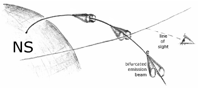
Figure 1: The principle of creating double features in radio pulse profiles: the line of sight traverses through a split-fan emission pattern, produced by outflowing particles that emit a double-lobed beam. For simplicity, the figure shows only a single trajectory of electrons flowing in a stream of finite width.

When the double-lobed beam is carried along with the electron, a split-fan beam is created, as shown in Fig. 1. In this paper we show that when the line of sight cuts through the stream at an oblique angle, a specific change of the BEC’s shape is expected across the frequency spectrum (Section 2). The resulting asymmetry of the BEC allows for a piece-wise fitting of double notches with a physical beam-shape model (Section 3).

One important difference between the stream-cut origin of components and the conal view of profile formation is the following: the altitude of detectable emission corresponds to that part of the stream, which is nearly tangential to the line of sight, whereas in the conal model, the altitude is fixed by a preselected value of $\nu$ (the tangency condition determines the azimuth of detectable region, but not the altitude). In the case of the stream-cut scenario, when the line of sight is not in the plane of the radio-emitting stream, no (or little) radiation is detectable, irrespective of $\nu$. When the sightline crosses the stream plane, only a localized piece of the stream is detectable, namely, the part that happens to be (nearly) tangent to the line of sight. Thus, the ‘observable’ altitude is frequency-independent, because the condition for tangency does not depend on the frequency of observation. Consequently, if the components observed in pulse profiles arise from stream cutting (whether they appear double, or single because of convolution effects), they will not exhibit the radius-to-frequency mapping (RFM). That is, the components will remain at fixed, frequency-independent locations in pulse profiles observed at different $\nu$.

Such a stream-cut origin of components allows us then to explain the lack of RFM in millisecond pulsars (MSPs; Kramer et al. 1999). Stream-cut viewing geometry is more likely in MSPs, because the polar cap of MSPs is much larger than for normal pulsars. Therefore, any transverse motion of limited magnitude, like the $\vec{E}\times\vec{B}$ drift, is less likely to create the hollow-cone emission pattern. Moreover, magnetic field lines in the MSPs flare strongly away from the dipole axis, which facilitates cutting of sightline through streams.

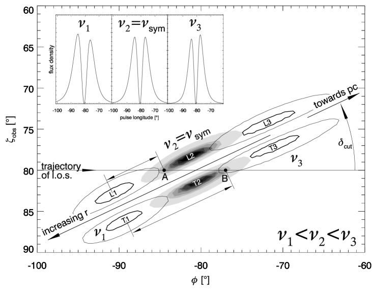
Figure 2: Origin of asymmetry inversion in bifurcated components of pulsar profiles. The three pairs of contours present sky-patterns of flux at three frequencies $\nu_{1}<\nu_{\rm sym}<\nu_{3}$. The patterns result from emission of a stream extending quasi-diagonally towards the bottom-left corner of the graph. Observer’s line of sight crosses the stream along the horizontal line. For more details see Section 2.

2 Oblique cut through split-fan beams

The split-fan emission of a stream, when projected on the sky, creates an elongated double track, such as the slanted pattern shown in Fig. 2. There, the sky-projected emission is presented at three frequencies: $\nu_{1}$ (two left contours: L1, and T1), $\nu_{2}$ (grey central contours: L2, T2), and $\nu_{3}$ (two right-hand side contours: L3, T3). For clarity of the figure, the contours mark only the brightest (topmost) parts of the emission pattern. There is actually considerable (and detectable) level of emission extending all the way across the figure at each frequency. Passage of sightline through the pattern, eg. along the horizontal line in Fig. 2, results in essentially double shape of observed component, regardless of the frequency of observation (see the triple inset). Assuming some residual RFM, for decreasing $\nu$ the double track has a maximum at increasing distances from the polar cap, ie. the location of the peak flux moves from right to left in Fig. 2. For appropriate traverse of sightline, there exists a frequency (denoted $\nu_{2}$ in Fig. 2, and hereafter called the frequency of symmetry, $\nu_{\rm sym}$), at which both maxima in the BEC have the same peak flux. Note that for non-orthogonal cuts ($\delta_{\rm cut}\neq 90^{\circ}$) through the split pattern, the line of sight does not cross through the maxima of the $\nu_{\rm sym}$-pattern (marked ‘L2’ and ‘T2’ in the figure). Even at this frequency of symmetry the sightline misses the leading maximum L2, moving on the ‘far side’ of it. That is, the sightline passes through the stream at a larger radial distance $r_{\rm A}$ than that of the peak emission: $r^{\rm max}(\nu_{2})\equiv r^{\rm max}_{2}<r_{\rm A}$. The trailing maximum of the $\nu_{2}$-pattern is passed-by at $r_{\rm B}<r^{\rm max}_{2}$, ie. below the radial distance of peak flux at this frequency. Thus, even when peaks of an observed BEC have perfectly the same-height, they nevertheless correspond to different emission altitudes (for $\delta_{\rm cut}\neq 0$). For this reason, despite having equally high peaks at $\nu_{\rm sym}$, the observed BEC will not be ideally symmetric: the peaks can have somewhat different widths due to a difference in curvature radii (see below).

At a lower frequency $\nu_{1}<\nu_{\rm sym}$ the BEC will have the leading peak brighter than the trailing one, because our line of sight passes closer to the leading maximum in the $\nu_{1}$ pattern (L1). Using the markings of Fig. 2, at frequency $\nu_{1}<\nu_{\rm sym}$ we have $|\rm{L1\ A}|<|\rm{T1\ B}|$. This holds (ie. the leading peak is the brighter one at ‘subsymmetric’ frequency) if the polar cap (region of lower altitudes) is located on the right-hand side (trailing side) of the observed feature, as in Fig. 2. That is, the leading peak is expected to dominate at $\nu<\nu_{\rm sym}$ if the BEC is observed as a precursor; for a ‘postcursor’ position of the BEC, the opposite is expected: a brighter trailing peak at $\nu<\nu_{\rm sym}$.

Conversely, the trailing peak of a BEC becomes brighter at $\nu_{3}>\nu_{\rm sym}$, because $|\rm{A\ L}3|>|\rm{B\ T}3|$, see Fig. 2. Thus, when the BEC is inspected at increasing frequencies, the dominating (brighter) peak switches from the leading to trailing position at $\nu_{\rm sym}$ (see the inset of Fig. 2). Observations of Kramer et al. 1999 (fig. 5 therein) provide evidence of such behaviour in J1012$+$5307. For the precursor location of the BEC, it is the leading peak which is expected to be brighter at low $\nu$, again in consistency with the profile of J1012$+$5307.

2.1 Asymmetry of the width at $\nu_{\rm sym}$

At the “frequency of symmetry” the maxima of BEC have precisely equal height, but the symmetry is approximate, because their widths are slightly different. The reason for this is that the width-scale of the BEC also depends on the curvature of trajectory of electrons flowing in the stream (in addition to the dependence on $\delta_{\rm cut}$). Low in the dipolar field, the curvature radius $\rho$ increases with altitude, as a result of which the emitted beam becomes narrower. The leading half of the BEC originates from larger altitudes (see Fig. 2) and should therefore be narrower than the trailing part, for which the altitude and $\rho$ are smaller. Assuming the oblique cut and the normal RFM, the bifurcated precursors are then expected to have the leading wing narrower than the trailing one. Weak traces of such asymmetry can be discerned in the BEC of J1012$+$5307 (see fig. 4 in DRD10).

This inference has been verified with a numerical code that follows beam-resolved emission of electrons moving along narrow streams in rotating dipolar magnetosphere. In the numerical calculations illustrated in Figs. 3 and 4, we assume that the B-field has the geometry of the rotating retarded vacuum dipole as given by equations A1 – A3 in Dyks & Harding (2004). Thus, we do not take into account the modifications of $\vec{B}$, that are expected for plasma-filled magnetosphere (see eg. Bai & Spitkovsky 2010 for the force-free case). The usual static-shape dipole is assumed only for the analytical calculations of Section 2.2.2 and Fig. 5. In the calculations that have led to Figs. 3 and 4, the local beam of non-coherent curvature radiation is emitted, with the realistic size appropriate for a preselected frequency $\nu$, and for local $\rho$ (as measured in the inertial observer’s frame IOF). However, instead of using the bandwidth-integrated beam, in Figs. 3 and 4 we have used the ‘bolometric beam’ which is integrated over the entire frequency spectrum. This is because: 1) the bolometric beam is given by the simple analytical formula of eq. 8 in DRD10, and 2) the shape of the bolometric beam happens to be similar to the observed shape of the BEC in J1012$+$5307, despite the latter is bandwidth-limited only. In this way we have avoided some deeply-nested calculation loops that would have otherwise been required to perform bandwidth-limited integration of the frequency-resolved beam, which cannot be expressed in a simple analytical way. Such a realistic beam shape (ie. one which corresponds to the observed bandwidth) is only used in Section 3 to fit the double notches of B1929$+$10. The Lorentz factor $\gamma$ in the bolometric beam is set to a value that corresponds to the realistic opening angle of bandwidth-limited beam at the central frequency of $\nu=820$ MHz, and which also corresponds to the local IOF curvature radius of electron trajectory. [Note: In the low-frequency limit, ie. when the BEC’s spectrum extends to much higher frequency than the observation frequency $\nu$, the frequency-resolved beam of curvature radiation does not depend on the Lorentz factor, so the observation frequency and the curvature of trajectory fully define the opening angle.] Thus, whereas the shape of the beam used for calculations illustrated in Figs. 3 and 4 is approximate, its opening angle is a realistic one. The aberration and propagation time effects (for flat space-time) are included in these calculations.

Note that on the LS of polar cap, the IOF radius of curvature increases with the radial distance $r$ at a slower rate than the standard dipolar radius of curvature $\rho_{\rm dip}$. The latter is equal to:

$$\rho_{\rm dip}\simeq\frac{4}{3}\frac{\sqrt{rR_{\rm lc}}}{s},$$ (1)

where $s=\sin\theta_{m}/\sin\theta_{lo}$ is the fieldline footprint parameter, $\theta_{m}$ is the magnetic colatitude (measured from the dipole axis), $\theta_{lo}$ is the magnetic colatitude of the last open field lines at radial distance $r$, and $R_{\rm lc}$ is the light cylinder radius. The corresponding radius of curvature of electron trajectory in the IOF is:

$$\rho\simeq R_{\rm lc}\negthinspace\left(\frac{3}{4}\frac{s}{\sqrt{r/R_{\rm lc}}}+2\sin\alpha\right)^{\negthinspace\negthinspace-1}\negthinspace\negthinspace\negthinspace=R_{\rm lc}\negthinspace\left(\frac{R_{\rm lc}}{\rho_{\rm dip}}+2\sin\alpha\right)^{\negthinspace\negthinspace-1}\negthinspace\negthinspace\negthinspace\negthinspace\negthinspace\negthinspace.$$ (2)

This equation only refers to the leading side of polar tube and holds when the viewing angle $\zeta$ is equal to the dipole inclination ($\alpha\simeq\zeta$). Comparison of eqs. (1) and (2) tells us that the increase of radius of curvature with altitude is smaller for the electron trajectory, than it is for the corresponding B-field line along which the electron moves in the corotating frame CF. For the orthogonally-rotating MSP with $P=5.25$ s ($R_{\rm lc}=25\cdot 10^{6}$ cm), the dipolar radius of curvature at the leading side of polar cap is $\rho_{\rm dip}=6.7\cdot 10^{6}$ cm, whereas the radius of curvature of the corresponding IOF trajectory is equal to $\rho=4.3\cdot 10^{6}$ cm. In our numerical code, the IOF values of $\rho$ are used. Within a limited part of magnetosphere they are given by eq. (2) (Dyks, Wright & Demorest 2010; Thomas & Gangadhara 2005).

Figure 3: Frequency evolution of a BEC, calculated for $\alpha=\zeta=85^{\circ}$, $\phi_{m}=95^{\circ}$, $s=1.2$, $P=5.26$ ms. The extent of emissivity along the electron path was $\Delta l=0.1R_{\rm lc}$ and the RFM was $r\propto\nu^{-0.13}$. Note the asymmetry inversion, and the increase of $\Delta$ for decreasing $\nu$. This BEC is created by the viewing geometry represented by the lowest horizontal line in the next figure.

A sample result, presented in Fig. 3, has been obtained for an almost orthogonal rotator, with dipole tilt of $\alpha=85^{\circ}$, $\zeta=85^{\circ}$, $P=5.25$ ms, $\nu=0.5$, $0.8$, and $1.4$ GHz. The stream was infinitesimally thin and constrained to a single B-field line with the footprint parameter $s=1.2$ and the surface magnetic azimuth $\phi_{m}=95^{\circ}$. For the model of Fig. 2 to work, the radial profile of emissivity may be represented by any non-monotonic function of altitude, with a single maximum at some height. A convenient function that we had arbitrarily selected was the Gauss function of the IOF length of electron path (measured along their IOF trajectory). The emissivity had a maximum at some ‘path-tracing’ distance of $l_{\rm max}$ from the polar cap, and the $1\sigma$ width of the emissivity profile was equal to $\Delta l=0.1R_{\rm lc}$. A weak, residual RFM of $r\propto\nu^{-0.13}$ was assumed, ie. the peak emissivity for the frequencies $\nu=0.5$, $0.8$ and $1.4$ GHz occurred at distances of $0.31$, $0.29$, and $0.27R_{\rm lc}$ from the polar cap.

Results of the simulations shown in Fig. 3 confirm the expectations based on Fig. 2: because of the RFM, the ratio of fluxes in the two peaks becomes inverted, but the BEC stays fixed at the same pulse phase at all frequencies. The separation of maxima in the BEC increases for decreasing frequencies ($\Delta_{\rm bfc}\propto\nu^{-1/3}$), which is caused purely by intrinsic properties of the emitted microbeam; it is not caused by the RFM. The trailing half of the simulated BEC is wider than the leading one (if both are measured at half maxima). This results from the fact that the leading part of the BEC on average originates from a larger $r$ than the trailing part (see Fig. 2). In the simulation shown, the asymmetry of width amounts to $\sim 4$%, which is noticeably larger than observed for J1012. A close inspection of fig. 8 in DRD10 reveals asymmetry of width of $\sim 1$% magnitude. This may suggest that the BEC of J1012 originates from non-dipolar (more circular) B-field lines, or that the cut angle $\delta_{\rm cut}$ is larger than in the simulation (or both).

The degree of asymmetry of peak flux at $\nu\neq\nu_{\rm sym}$, depends in a degenerate way on several factors, such as $\Delta l$, $\delta_{\rm cut}$, and the strength of RFM. To measure the flux asymmetry, let us introduce the ratio $R_{F}=F_{l}/F_{t}$, where $F_{l}$ and $F_{t}$ denote the peak flux at the leading and trailing maximum in the BEC. At frequencies far from $\nu_{\rm sym}$ the ratio $R_{F}$ can evolve with $\nu$ or stay constant, depending on the radial profile of emissivity. This is because for a fixed viewing geometry $R_{F}$ simply represents the ratio of emissivities at two fixed altitudes: $R_{F}(\nu)=F_{\nu}(r_{\rm A})/F_{\nu}(r_{\rm B})$, where the indices ‘A’ and ‘B’ refer to the points in Fig. 2.

For small values of $\Delta l$ or $\delta_{\rm cut}$ the asymmetry $R_{F}$ strongly depends on the viewing angle $\zeta$, which can vary as a result of precession, as well as on $\alpha$. A change of $\zeta$ by just $1^{\circ}$ (from the value of $85^{\circ}$ shown in Fig. 3, to $\zeta=84^{\circ}$) changes the flux ratio from $R_{F}\sim 1$ (Fig. 3b) to $R_{F}\sim 0.4$. With the additional asymmetry in the width of the peaks, such components would probably be not identified as ‘bifurcated’ at all (they look just ‘double’).

2.2 Apparent magnification by geometric effects

The double features can be interpreted as a direct consequence of structured shape of microscopic emission beam. Let us consider that part of the curvature radiation beam which is polarised orthogonally to the plane of electron trajectory. Let the frequency of observation be much smaller than the peak frequency $\nu_{\rm crv}$ of standard curvature spectrum: $\nu_{\rm crv}=7\ {\rm GHz}\ \gamma^{3}/\rho\rm[cm]$, where $\gamma$ is the electron Lorentz factor. Radiation of this type has the intrinsic bifurcation angle of:

$$2\psi=0.8^{\circ}(\rho_{7}\nu_{9})^{-1/3},$$ (3)

where $\rho_{7}=\rho/(10^{7}\ {\rm cm})$, and $\nu_{9}=\nu/(1\ {\rm GHz})$. For dipolar curvature radii $\rho_{7}\sim 1$, the beam is up to 10 times narrower than the size of features observed in B0950, B1929, and J1012. If the physical model is correct, it implies that either $\rho\sim 10^{4}-10^{5}$ cm, or that the observed width has been strongly enlarged by geometrical magnification.

2.2.1 Probability of small-angle cut through the stream

To illustrate the effects of geometrical enlargement, we have calculated a sky pattern of bifurcated emission from 72 streams that emerge from the surface of neutron star at equal intervals of magnetic azimuth $\Delta\phi_{m}=5^{\circ}$. The result is shown in Fig. 4, where the bifurcated nature of the emission can be discerned as a low-flux fissure at the centre of each emission stripe. We have selected B-field lines with the footprint $s=1.2$ to maximize the bifurcation angle (so it is more easily discernible in the figure) as well as to avoid some overlapping and pile-up of emission due to the caustic effects (which tend to occur for $s\la 1$). The most vertical emission stripes correspond to $\phi_{m}=190^{\circ}$ (the top one), and $\phi_{m}=350^{\circ}$ (bottom). The radial emissivity profile was the Gauss function with $l_{\rm max}=0.25R_{\rm lc}$ and $\Delta l=0.1R_{\rm lc}$. The three horizontals mark sightline traverse at $\zeta=20$, $50$, and $85^{\circ}$. The dipole tilt was $\alpha=85^{\circ}$ so the radiation from the magnetic pole is located in Fig. 4 at $\phi=-2R_{\rm NS}/R_{\rm lc}=-4.5^{\circ}$, $\zeta=85^{\circ}$.

As can be seen in Fig. 4, with increasing distance from the polar cap the emission of streams tends to assume horizontal direction and the stripes of emission are cut at small angles by the line of sight. Far away from the pole ($|\phi|\sim 90^{\circ}$) this is true for any viewing angle $\zeta$. For $\zeta\simeq\alpha$, the cut angle is small within the entire phase range shown in Fig. 4, except from the close vicinity of $\phi=0$. For small $\zeta\sim 20^{\circ}$ the observed bifurcation is large for any phase, because of the classical magnification by the ‘not a great circle’ effect. Thus, for the case shown in Fig. 4, it is only for moderate viewing angles $\zeta\sim 30-60^{\circ}$, and for a limited range of phase $|\phi|<70^{\circ}$, where the BECs are not strongly magnified. Moreover, if we assume that easily-detectable pulsars are viewed at a small impact angle ($\zeta\simeq\alpha$), then the strong enlargement should be expected for a wide phase interval. This is because in this case the cut angle $\delta_{\rm cut}$ is noticeably large only for limited phase range around $\phi\sim 0$, and $\phi\sim 180^{\circ}$ (see the dashed line for $\zeta=75^{\circ}$ in Fig. 5 further below).

We conclude that there is a fairly large parameter space in which the observed width of BECs can be considerably increased by geometric effects of either 1) the small cut angle $\delta_{\rm cut}$, or 2) the small viewing angle $\zeta$. The presence of the first factor considerably increases the size of the space, in comparison to the case of conal beam, for which only the second type of enlargement was possible.

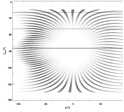
Figure 4: Sky-projected emission from 72 streams with $s=1.2$ and $\phi_{m}=0^{\circ}$, $5^{\circ}$, $10^{\circ}$, $15^{\circ}$, etc. For all streams $l_{\rm max}=0.25R_{\rm lc}$ and $\Delta l=0.1R_{\rm lc}$. The other parameters are the same as in the previous figure. Note the bifurcated nature of the emission stripes, and their tendency to assume horizontal direction at large $|\phi|$, that results in a small cut angle $\delta_{\rm cut}$.

2.2.2 Peak separation as a function of viewing geometry

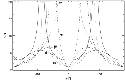
Figure 5: Observed separation of peaks in a double feature produced by the sightline’s traverse through a split-fan emission beam with bifurcation of $2\psi=1^{\circ}$. Curves of different types are calculated from eq. (4) with $\alpha=80^{\circ}$, for six values of $\zeta=20^{\circ}$ (solid), $50^{\circ}$ (dotted), $75^{\circ}$ (dashed), $80^{\circ}$ (dot-dashed), $85^{\circ}$ (three-dot-dashed), and $90^{\circ}$ (long-dashed). Note the obvious possibility of observing $\Delta>5^{\circ}$ within $|\phi|<120^{\circ}$, despite $\psi=0.5^{\circ}$.

If the aberration and retardation are neglected, the apparent separation $\Delta$ of maxima in a BEC can be derived by application of spherical trigonometry to the standard dipolar magnetic field. The result is:

$$\cos{\left(\frac{\Delta}{2}\right)}=\frac{\cos\kappa-\cos^{2}\zeta}{\sin^{2}\zeta},$$ (4)

where

$$\sin{\kappa}=\frac{\sin{\psi}}{\sin\delta_{\rm cut}}.$$ (5)

The bifurcation angle $2\psi$ is given by eq. (3), whereas the cut angle $\delta_{\rm cut}$ is equal to:

$$\delta_{\rm cut}=90^{\circ}-\psi_{\rm PA},$$ (6)

where $\psi_{\rm PA}$ is the usual polarisation angle between the sky-projected B-field and the sky-projected rotation axis:

$$\tan\psi_{\rm PA}=\frac{\sin\alpha\sin(\phi-\phi_{0})}{\cos(\phi-\phi_{0})\cos\zeta\sin\alpha-\cos\alpha\sin\zeta}$$ (7)

(Radhakrishnan & Cooke 1969). Equation (4) is the split-fan analogue of the well-known equation for opening angle of conal beams. When the bifurcation angle $2\psi$, and the observed separation $\Delta$ are small, eq. (4) reduces to:

$$\Delta\simeq\frac{2\psi}{\sin\zeta\sin\delta_{\rm cut}}$$ (8)

as was guessed in DRD10.

With the special relativistic (and altitude-sensitive) effects ignored, the cut angle $\delta_{\rm cut}$ is uniquely determined for every pulse phase $\phi$ as soon as $\alpha$, $\zeta$ and $\phi_{0}$ are selected. Therefore, eq. (4) actually gives the separation $\Delta$ as a function of pulse phase $\phi$. Fig. 5 presents examples of such curves calculated for $\alpha=80^{\circ}$, $\psi=0.5^{\circ}$, and various viewing angles $\zeta$. It can be seen that for $\zeta<\alpha$ our sightline’s traverse becomes instantaneously tangent to the projected B-field lines, which causes $\Delta$ to increase infinitely. For small $\zeta\ll\alpha$ this happens near $|\phi|\sim 90^{\circ}$ whereas for $\zeta$ approaching $\alpha$ this phase interval moves closer to the dipole axis phase at $\phi=0$.

In spite of the rather small intrinsic bifurcation of $2\psi=1^{\circ}$, the observed bifurcation $\Delta$ can reach large values within wide phase intervals that precede and lag the phase of dipole axis. If measured from the brightest (main) feature in a pulse profile, the known double features are located at phase longitudes: $103.5^{\circ}$ (B1929$+$10), $51^{\circ}$, $70^{\circ}$ (J0437$-$4715), $-30^{\circ}$ (B0950$+$08), $-55^{\circ}$ and $130^{\circ}$ (J1012$+$5307). As can be seen in Fig. 5, all these numbers, except from the last one, lay within the phase interval of strong magnification. Unfortunately, it is the last location which corresponds to the bright BEC of J1012$+$5307, the widest-observed so far. However, even this case can be accounted for by the model, if the dipole inclination $\alpha$ in J1012$+$5307 is very small or close to $90^{\circ}$ (in the latter case the phase $\phi=130^{\circ}$ becomes equivalent to $\phi=-50^{\circ}$, and there is no difference between the main pulse and interpulse).

2.2.3 Possibility of interpulses

Regions of strong radio emission in pulsar magnetosphere are definitely more localised than shown in Fig. 4, because the observed profiles usually have duty cycles much smaller than $360^{\circ}$. However, most of the emission that contains double features is not localized within a narrow range of phase. This is the case of B1929$+$10, B0950$+$08, and J0437$-$4715. Narrow radio pulses become a possibility when azimuthal limitations for the extent of emission are allowed, or when the radial extent of strong emissivity is not too large, yet noticeable, say $\Delta r\la 0.1R_{\rm lc}$.

It is worth to note that even for very extended emission regions, interpulses do not have to be always detectable, because of bulk topological properties of pulsar magnetosphere. One example of this is the outer gap model, in which ‘the other pole’ emission is undetectable by a single observer because it is constrained to regions above the null-charge surface (Romani & Yadigaroglu 1995; Wang et al. 2011). Another example is the slot gap model (Arons 1983; Muslimov & Harding 2003) with the large-scale acceleration possible only on favourable (poleward) magnetic field lines. Thus, in a large fraction of existing magnetosphere models the invisibility of the other pole is an inherent property. It is therefore possible that radially-extended emission streams are present in many objects, but are not directly manifested by unavoidable second-pole emission.

3 Piece-wise fits of physical curves to the double notches

As can be seen in Fig. 2, the altitude of detectable emission changes gradually while the sightline is obliquely traversing through the double pattern. Therefore, the width and height of the sampled microbeam also gradually change with pulse phase, because they depend on the curvature radius $\rho(r)$ and $r$-dependent emissivity. Obviously, the same is true for double features in the absorption version, ie. for double notches which may have $r$-dependent width and depth. Precise fits to double features then require a full 3D modelling of the stream-cut geometry, ie. the $r$-dependence of the depth of the notches, and the $r$-dependence of $\rho$ need to be assumed in addition to $\alpha$, $\zeta$, and the specific functional form of the microbeam. This kind of calculation is feasible with the code of type that produced the result shown in Fig. 4. However, the frequency-integrated (bolometric) microbeam which is now used by the code, would need to be replaced by an observing-band-integrated beam. And the code would have to be embedded into a fitting routine with some iterative capability of heading towards $\chi^{2}$ minimum. Instead of these numerical developments, we make a direct, but piece-wise fit to the double notches of B1929$+$10 using the bandwidth-integrated beam. More precisely, it is assumed that the left half of the notches on average originates from some unspecified altitude with one curvature radius $\rho(r_{A})$, and the other half on average originates from another altitude and $\rho(r_{B})$. Since the scale of the fitted beam depends only on the curvature radius $\rho$, it is only the values of $\rho_{i}$ that are provided by the fit. Any further association of $\rho_{i}$ with radial distances $r_{i}$ is not unique because of unknown viewing geometry ($\delta_{\rm cut}$). As will be seen below, the limited quality of the best-available data on the notches of B1929$+$10, makes this procedure reasonable, because fractional values of $\chi^{2}/dof$ can be reached even with this simplified model.

3.1 Functional form of the fitted microbeam

The radio flux at pulse longitudes surrounding the notches of B1929$+$10 changes linearly (see fig. 1 in DRR07). Therefore, before making the fit we remove this linear trend to get a constant flux normalised to unity (Fig. 6). Then we use the following function to fit the data:

$$I(\phi)=1-\int\limits^{\nu_{\rm max}}_{\nu_{\rm min}}\eta_{\rm crv}\ d\nu,$$ (9)

where the integration is over the observed frequency bandwidth and $\eta_{\rm crv}$ represents the shape of curvature radiation microbeam:

$$\eta_{\rm crv} = \eta_{\parallel}+\eta_{\perp}=$$ (10)

$$= \frac{q^{2}\omega^{2}}{3\pi^{2}c}\left(\frac{\rho}{c}\right)^{2}\left[C_{\parallel}\xi^{2}K^{2}_{\frac{2}{3}}(y)\ +\right.$$ (11)

$$+ \left.C_{\perp}\xi\ K^{2}_{\frac{1}{3}}(y)\sin^{2}\psi\right],$$ (12)

where

$$\xi=1/\gamma^{2}+\psi^{2},\ \ {\rm and}$$ (13)

$$y=\frac{\omega\rho}{3c}\xi^{3/2}$$ (14)

(eg. Jackson 1975). The symbol $\rho$ denotes the radius of curvature of electron trajectory in the IOF, $\omega=2\pi\nu$, $c$ is the speed of light, and $K$’s are the modified Bessel functions. The angle $\psi$ is the azimuth of the line of sight measured in a frame with z-axis along the instantaneous acceleration vector (it is the azimuth of sightline measured around the vector of curvature radius). The two terms in the square bracket represent decomposition of the beam into two parts: one polarised parallel, and the other polarised orthogonally to the plane of electron trajectory. In the absence of the parallel mode the normalisation constant $C_{\parallel}$ is equal to zero, and the microbeam has the double-lobed shape with zero flux in the centre. Therefore, if spatial convolution effects are not included in the fit, the central maximum of the double notches, which does not reach the ‘off-notch’ level, is not well reproduced (Fig. 6a, with $\chi^{2}/dof=1.1$ for the left notch, and $\chi^{2}/dof=0.6$ for the right notch). The decreased flux at the central maximum probably results from some convolution effects, such as the non-zero width of the non-emitting/eclipsing region. To avoid the complexity of such convolution (eg. the selection of transverse plasma density profile), we instead lower down the maximum by adding a bit of the parallel mode ($C_{\parallel}\simeq 0.13C_{\perp}$, Fig. 6b), which has a single-peaked pencil-like shape. Note that the data may well contain no parallel mode at all. We simply use the non-zero value of $C_{\parallel}$ as a convenient way to improve the fit. The spatial convolution seems to be the most natural explanation for the low flux at the center of ‘W’. In the fitting procedure we simply set $\psi=\phi-\phi_{c}$, where $\phi_{c}$ is the phase of the centre of the ‘W’. In the low-frequency limit of $\nu\ll\nu_{\rm crv}$, the shape and size of curvature radiation beam do not depend on the Lorentz factor $\gamma$ of emitting particles. Since the frequency of observation shown in Fig. 6 is relatively low ($\nu=327$ MHz), it is reasonable to perform the fitting without any reference to $\gamma$. To minimize the number of fit parameters in this way, we simply set $\gamma$ to some ‘very high’ value (eg. $10^{7}$) to ensure that $\nu\ll\nu_{\rm crv}(\gamma,\rho)$. The width scale of the beam is then changed only through changes of $\rho$. Therefore, the fitted value of curvature radius also incorporates any influence of viewing geometry on the scale of the notches. Thus, the fit actually provides us with the value of $\rho_{\rm min}=\rho\sin^{3}\zeta\sin^{3}\delta_{\rm cut}$, where the subscript ‘min’ has the meaning of minimum value of $\rho$ for both $\zeta$ and $\delta_{\rm cut}$ equal to $90^{\circ}$. In spite of the wide bandwidth ($\Delta\nu/\nu=8\%$), the frequency integration in eq. (9) does not change the beam shape considerably. The bandwidth-integrated beam stays similar to the frequency-resolved shape of eq. (12).

Figure 6: A fit of classical curvature radiation beam (eq. 9) to double notches in the 327-MHz pulse profile of B1929$+$10. Each notch is fitted separately, within the left-hand side, and right-hand side pair of solid vertical lines. The pair of dotted verticals marks the phase interval used to remove the linear increase of flux with phase. In panel a) the orthogonal polarisation mode is only used ($C_{\parallel}=0$). In panel b) we have fixed $C_{\parallel}\simeq 0.13\ C_{\perp}$ to match the central data points. The data were collected with the Arecibo Telescope (DRR07); the bandwidth was $25$ MHz.

As can be seen in Fig. 6, the curvature radiation beam reproduces the notches of B1929$+$10 very well. Even when no account is done for the lowered flux of the central minimum (Fig. 6a), the shape of the curvature subbeam neatly reflects the steepness of the outer walls of the ‘W’, as well as the bulk width of the minima, as compared to the separation between them. With the central maximum lowered down for the price of one additional fit parameter ($C_{\parallel}$), the quality of the fit reaches $\chi^{2}/dof=0.7$ and $0.2$ for the left and right-hand side notch respectively (Fig. 6b).

3.1.1 Curvature radii

The fitted values of curvature radius are: $\rho_{\rm min}=1.17$, and $0.85\cdot 10^{5}$ cm for the leading and trailing notch, respectively. These values assume orthogonal and equatorial cut through the stream ($\delta_{\rm cut}=\zeta=90^{\circ}$) and should be understood as the lower limits for $\rho=\rho_{\rm min}/(\sin^{3}\zeta\sin^{3}\delta_{\rm cut})$. The value of $\rho_{\rm min}$ fitted for the leading notch is somewhat larger than for the trailing one. This seems to be natural for the double notches of B1929$+$10, because small $\delta_{\rm cut}$ is likely for this object: the interpulse suggests that $\alpha\sim\zeta\sim 90^{\circ}$, and the notches are located $103.5^{\circ}$ after the main pulse, ie. within the region of strong amplification through the small-$\delta_{\rm cut}$ effect (Fig. 5). Note that already for moderately small $\delta_{\rm cut}=28^{\circ}$ (and $\zeta=90^{\circ}$), the inferred value of $\rho$ reaches $10^{6}$ cm, whereas for $\delta_{\rm cut}=13^{\circ}$, $\rho=10^{7}$ cm. The fitted size of the double notches ($\Delta=5.37^{\circ}$ at $\nu=327$ MHz) is then compatible with dipolar values of near-surface $\rho$ in the closed field line region.

In the plane of the magnetic equator the curvature radius of dipolar B-field lines is equal to:

$$\rho_{eq}\equiv\rho(\theta_{m}=90^{\circ})=\frac{r}{3},$$ (15)

where $\theta_{m}$ is the magnetic colatitude of the emission point, measured from the dipole axis. Thus, for every pulsar with radius $R_{ns}=10^{6}$ cm, the minimum curvature radius available in its dipolar magnetosphere is equal to $\rho=3.3\cdot 10^{5}$ cm.

In B1929$+$10 the double notches are observed at $\phi\simeq 103.5^{\circ}$, ie. roughly at the right angle with respect to the dipole axis. Therefore, it is useful to find the surface value of $\rho$ at the position where the B-field is pointing at the right angle $\theta_{B}=90^{\circ}$ with respect to the dipole axis. The magnetic colatitude for this point is equal to $\theta_{m}\simeq 54.73^{\circ}$ (more precisely: $\sin^{2}\theta_{m}=2/3$), and the corresponding curvature radius is:

$$\rho_{\perp}\equiv\rho(\theta_{B}=90^{\circ})=\frac{\sqrt{3}}{2}\thinspace r,$$ (16)

which at the star surface gives $\rho=0.866R_{ns}\simeq 10^{6}$ cm. Thus, even in the presence of only modest geometrical amplification ($\delta_{\rm cut}\simeq 30^{\circ}$, $\zeta\simeq 90^{\circ}$) the dipolar curvature radii in the closed field line region are consistent with the observed width of double notches in B1929$+$10.

In the unlikely case of large $\delta_{\rm cut}$, the substellar values of $\rho_{\rm min}$ would have to be interpreted in terms of small-scale distortions of dipolar B-field (Harding & Muslimov 2011; Ruderman 1991). Another option, at least in principle, would be the gyration radius of primary particles near the light cylinder:

$$r_{B}=1702\ {\rm cm}\ \frac{m}{m_{e}}\frac{\gamma}{B},$$ (17)

where $m/m_{e}\equiv m^{\prime}$ is the mass of radiating charges in units of the electron mass $m_{e}$, and $B$ is in Gauss. This radius translates into the bifurcation angle of:

$$2\psi=14.4^{\circ}\left(\frac{B{\rm[G]}}{m^{\prime}\gamma\nu_{9}}\right)^{1/3},$$ (18)

which is broadly consistent with observations for $B\la 10^{5}$ G and $\gamma\ga 10^{6}$. However, to produce strong and unsmeared double features, the gyrational motion would have to be spatially ordered within a large volume of magnetosphere. This does not immediately seem to be natural.

3.2 Separation as a function of frequency

In view of the remarkable agreement seen in Fig. 6, it is needed to verify if the separation $\Delta$ between the minima (or maxima) in double features is also consistent with the properties of curvature radiation. According to the classical electrodynamics, at low frequencies ($\nu\ll\nu_{\rm crv}$) the separation $\Delta$ decreases with increasing $\nu$ according to eq. (3), ie. according to the power-law $\Delta\propto\nu^{-a}$ with the index $a=1/3$. The bifurcation angle in this case is $\psi\gg 1/\gamma$, where $\gamma$ is the Lorentz factor of the emitting particles. At the high-energy end of the emitted spectrum, ie. within the high-energy spectral decline, the features merge faster, with the index $a=1/2$ (eg. Jackson 1975), and the bifurcation becomes very small: $\psi\ll 1/\gamma$. A simple arithmetic average then allows us to expect an ‘average’ merging rate of $a=0.417$ around the spectral maximum. It is worth to emphasize that many models of coherent curvature emission follow the same $\psi(\nu)$ as the non-coherent curvature radiation. Such models include those based on bunching of charges (Ruderman & Sutherland 1975), as well as some maser mechanisms (Luo & Melrose 1992; Kaganovich & Lyubarsky 2010),

The theoretical range of merging rate for the curvature radiation is compared to the available data on double features in Fig. 7, which includes data on both the emission (BEC) and absorption features (DN). The figure takes into account the new data on J0437$-$4715 from Yan et al. (2011), as well as unpublished low-frequency data on this object. For this reason the two points for J0437$-$4715 lay closer to $a=1/2$ than in fig. 6 in DRD10.

Figure 7: Average merging-rate index $a$ in the relation $\Delta\propto\nu^{-a}$. ‘BEC’ refers to bifurcated emission components, whereas ‘DN’ to double notches. Dashed verticals mark the range of $a$ expected if the doubleness is caused by the double-lobed microscopic beam of curvature radiation (eq. 9). The notches of B0950$+$09 (not included in this figure) are also consistent with $a=1/2$ (see fig. 9 in DRR07).

One can see that within the statistical $1\sigma$ errors, the measured merging rate is consistent with the one expected for the curvature beam. Inspection of $\Delta$ as a function of $\nu$ may even be revealing some decrease of $a$ at lower frequencies (see fig. 6a in DRR07). We remind here that it is not the merging rate that differentiates the curvature radiation from the other emission processes, because the latter can also have $a\la 1/2$ (eg. Melrose 1978; DRD10). However, if the origin of the observed doubleness is not related to the microscopic beam, this would possibly be manifested by merging index values from outside of the range $\left[1/3,1/2\right]$. The large number of indices near $a=1/2$ may be considered to be not quite natural for the curvature radiation, because double features should be more easily observable at low $\nu$, where the beam is wider, and the merging index $a$ is closer to $1/3$. However, double features at high $\nu$ can be more easily affected by blurring effects, which can also bring the maxima increasingly closer together, thus increasing $a$. We therefore conclude that the analysis of merging rate is broadly consistent with the curvature origin of double features.

3.3 Fitting the BEC of J1012$+$5307

We have also made several fits to the BEC of J1012$+$5307, in which the outer wings are much less steep than the outer wings of the double notches in B1929$+$10. Therefore, we have used functions that are a convolution of some bell-shaped plasma-density profile (like the Gauss or Lorentz functions) with the microbeam of eq. (9). This type of model has appeared to be unable to reproduce the BEC: before the flux in the wide outer wings has been reached, the flux in the central minimum was already too large. We conclude that with the use of the microbeam from eq. (9), the shape of the outer wings of the BEC in J1012$+$5307 cannot be reproduced by convolving it with bell-shaped density functions. Another convolution that is possible for the simple case of $\nu\ll\nu_{\rm crv}$, and which remains to be tried out, is a spread in curvature radii $\rho$, which can act similarly to the integration over a wide frequency range (much wider than the bandwidth). Yet another possibility is the case of $\nu\simeq\nu_{\rm crv}$, ie. the observation frequency being close to the characteristic frequency of curvature spectrum, in which case the opening angle is $\psi\sim 1/\gamma$, where $\gamma$ is the electron energy in units of $mc^{2}$. Finding the shape of BEC in such a case would require us to make integration over the electron energy distribution (in addition to the spatial convolution).

4 Conclusions

We conclude that the stream-cut geometry is a successful model for such components in radio pulse profiles like the apparently ‘conal’ components in J0437$-$4715, or the BEC in J1012$+$5307. Such geometry naturally explains the fixed, frequency-independent location of these features in the profiles. The components stay at a fixed phase not because of the ‘lack of RFM’, but because the emission region is narrow in azimuth (stream-like emitting region, or spoke-like, if there are more streams). If the RFM is added to this picture, it does not move the components away from the profile center. Instead, in the case of non-orthogonal cut through the stream, the RFM is making the double features asymmetric at all frequencies, except from at $\nu_{\rm sym}$. This conjecture is valid for stream-like emitters with RFM regardless of the actual origin of the doubleness, ie. regardless of whether the bifurcation has the micro- or macroscopic origin.

If we assume that the doubleness reflects the shape of the microphysical beam, then the curvature radiation in the extraordinary mode becomes a natural process, because: 1. it is intrinsically double-lobed (bifurcated), which is a necessary condition for producing deep double notches (DRD10); 2. the extraordinary part of the curvature beam reproduces the shape of notches in B1929$+$10; 3. the rate of merging of double features with increasing frequency is consistent with the curvature origin; 4. the width-scale of double features in B1929$+$10 and J0437$-$4715 is consistent with dipolar curvature radii; 5. the high polarisation of double features is consistent with the single-mode nature of the double-lobed beam.

This said, it is not quite clear why some of the observed double features have the width of $\ga 7^{\circ}$ at 1 GHz, despite the intrinsic beam is expected to be only $1^{\circ}$ wide. However, the quite large probability of strong geometric magnification, along with the possibility of smaller-than-dipolar $\rho$, do not really allow us to consider this issue as a serious problem for the curvature microbeam model. As recently noted by Yan et al. (2011), who verify fairly large sample of high-quality profiles of MSPs, bifurcated features are rare among MSPs. This is in line with the special requirements that need to be fulfilled for these features to be observable. The requirements apparently include at least the following: 1. the spatial extent (azimuthal width of the stream) must not be too large to blur the feature; 2. the feature be best magnified by geometrical effects to be wide and easily detectable. It is not clear why we do not observe features with $\Delta\la 1^{\circ}$, that fulfill the condition no. 1, but are not magnified geometrically. Generally, however, the intrinsic narrowness of the curvature beam seems to be consistent with the rarity of double features in the observed profiles. This is because for even a small azimuthal extent of emission region, the doubleness should become hidden by spatial convolution effects.

We conclude that the asymmetry of double features at different frequencies, the shape of notches in B1920$+$10, the way they merge, their high polarisation, and their fixed phase locations can all be understood in terms of sightline cuts through streams of plasma that emits curvature-radiation in the orthogonal polarisation mode.

References

- [1] Arons J., 1983, ApJ, 266, 215
- [2] Bai X.-N., Spitkovsky A., 2010, ApJ, 715, 1282
- [3] Dyks J., & Harding A. K., 2004, ApJ 614, 869
- [4] Dyks J., Fra̧ckowiak M., Słowikowska A., Rudak B., & Zhang B., 2005, ApJ 633, 1101
- [5] Dyks J., Rudak B., & Demorest P., 2010, MNRAS, 401, 1781 (DRD10)
- [6] Dyks J., Rudak B., & Rankin J. M., 2007, A&A, 465, 981 (DRR07)
- [7] Dyks J., Wright G.A.E., & Demorest P., 2010, MNRAS, 405, 509
- [8] Harding A.K., & Muslimov A.G., 2011, ApJ, 726, L10
- [9] Jackson J.D., 1975, “Classical Electrodynamics”, John Wiley & Sons Inc, New York
- [10] Kaganovich A., & Lyubarsky Y., 2010, ApJ, 721, 1164
- [11] Kramer M., Lange C., Lorimer D., Backer D.C., Xilouris K. M., et al., 1999, ApJ, 526, 957
- [12] Luo, Q., & Melrose, D. B. 1992, MNRAS, 258, 616
- [13] McLaughlin M. A., & Rankin J. M., 2004, MNRAS, 351, 808
- [14] Melrose, D.B. 1978, ApJ, 225, 557
- [15] Muslimov A. G., & Harding A.K., 2003, ApJ, 588, 430
- [16] Navarro J., Manchester R. N., Sandhu J. S., Kulkarni S.R., Bailes M., 1997, ApJ, 486, 1019
- [17] Perry, T.E., & Lyne, A. G. 1985, MNRAS, 212, 489 (PL85)
- [18] Radhakrishnan V., & Cooke D.J. 1969, Astrophys. Lett., 3, 225 (RC69)
- [19] Rankin J.M., & Rathnasree N., 1997, J. Astrophys. Astron., 18, 91
- [20] Romani R.W., & Yadigaroglu I.-A., 1995, ApJ, 438, 314
- [21] Ruderman M.A., 1991, ApJ, 366, 261
- [22] Ruderman M.A., Sutherland P.G. 1975, ApJ 196, 51
- [23] Thomas, R.M.C., & Gangadhara, R.T. 2005, A&A, 437, 537
- [24] Wang Y., Takata J., & Cheng K.S., 2011, MNRAS, 414, 2664
- [25] Wright, G. A. E., 2004, MNRAS, 351, 813
- [26] Yan W.M., Manchester R.N., van Straten W., Reynolds J.E., Hobbs G., et al. 2011, MNRAS, 414, 2087