Patterns of Regional Travel Behavior: An Analysis of Japanese Hotel Reservation Data

Abstract

This study considers the availability of room opportunities collected from a Japanese hotel booking site. We empirically analyze the daily number of room opportunities for four areas. To determine the migration trends of travelers, we discuss a finite mixture of Poisson distributions and the EM-algorithm as its parameter estimation method. We further propose a method to infer the probability of opportunities existing for each observation. We characterize demand-supply situations by means of relationship between the averaged room prices and the probability of opportunity existing.

1 Introduction

Recent technological development enables us to purchase various kinds of items and services via E-commerce systems. The emergence of Internet applications has had an unprecedented impact on our life style to purchase goods and services. From available data of items and services at E-commerce platforms, we may expect that utilities of agents in socio-economic systems are directly estimated.

Such an impact on travel and tourism, specifically, on hotel room reservations, is significantly considered (Law, 2009). According to Pilia (2008), 40 per cent of hotel reservations will be made via Internet in 2008, up from 33 per cent in 2007 and 29 per cent in 2006. Therefore, the coverage of room opportunities via the Internet may be sufficient to provide statistically significant results, and to conduct a comprehensive analysis based on the hotel booking data collected from Internet booking sites.

From our personal experience, it is found that it is becoming more popular to make reservations of hotels via the Internet. When we use a hotel booking site, we notice that we sometimes find preferable room opportunities or not. Namely, the hotel accessibility seems to be random. We further know that both the date and place of stay are important factors to determine the availability of room opportunities. Hence, the room availability depends on the calendars (weekdays, weekends, and holidays) and regions.

This availability of the hotel rooms may indicate the future migration trends of travelers. Therefore, it is worth considering accumulation of comprehensive data of hotel availability in order to detect inter-migration in countries.

The migration processes have been intensively studied in the context of socio-economic dynamics with particular interest for quantitative research. Weidlich and Haag proposed the Master equation with transition probabilities depending on both regional-dependent and time-dependent utility and mobility in order to describe collective tendency of agent decision in migration chance (Hagg & Weidlich, 1984).

Since the motivation of migration seems to come from both psychological and physical factors, the understanding of the dynamics of the migration is expected to provide useful insights on inner states of agents and their collective behavior.

In the present article, we discuss a model to capture behavior of consumers at a hotel booking site and investigate statistics of the number of available room opportunities from several perspectives.

This article is organized as follows. In Sec. 2, we give a brief explanation of data description collected from a Japanese hotel booking site. In Sec. 3, we show an outlook of collected data of the room opportunities. In Sec. 4, we consider a model to capture room opportunities and derive a finite mixture of Poisson distributions from binomial processes. In Sec. 5, we introduce the EM-algorithm to estimate parameters of the mixture of Poisson distributions. In Sec. 6, we computed parameter estimates for an artificial data set generated from the mixture of Poisson distributions. In Sec. 7, we show results of the empirical analysis on the room opportunities and discuss relationship between existing probabilities of opportunities and their rates. Sec. 8 is devoted to conclusions.

2 Data description

In this section, we give a brief explanation of a method to collect data on hotel availability. In this study, we used a Web API (Application Programing Interface) in order to collect the data from a Japanese hotel booking site named Jalan . Jalan is one of the most popular hotel reservation services which provide a WebAPI in Japan. The API is an interface code set which is designed for a purpose to simplify development of application programs.

Jalan Web service provides interfaces for both hotel managers and customers (see Fig. 1). The mechanism of Jalan is as follows: The hotel managers can enter information on room opportunities served by their hotels via an Internet interface. The consumers can book rooms from available opportunities via the Jalan Web site. The third parties can even built their web services with the Jalan data by using the Web API.

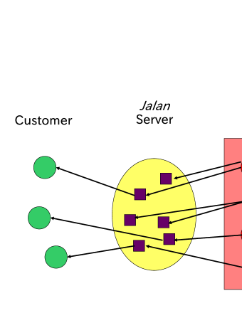
Figure 1: A conceptual illustration of Jalan web service. The hotel managers enter information on rooms (plans) which will be served at the hotels. Customers can search and book rooms from all the available rooms (plans) via Jalan web page.

We are collecting all the available opportunities which appear in Jalan regarding room opportunities in which two adults will be able to stay one night. The data are sampled from the Jalan net web site (http://www.jalan.net) daily. The data on room opportunities collected through Jalan Web API are stored as csv files.

In the data set, there exist over 100,000 room opportunities from over 14,000 hotels. In Tab. 1, we show contents included in the data set. Each plan contains sampled date, stay date, regional sequential number, hotel identification number, hotel name, postal address, URL of the hotel web page, geographical position, plan name, and rate.

Since the data contain regional information, it is possible for us to analyze regional dependence of hotel rates. Throughout the investigation, we regard the number of recorded opportunities (plan) as a proxy variable of the number of available room stocks.

Table 1: The data format of room opportunities.

Date of collection

Date of Stay

Hotel identification number

Hotel name

Hotel name (Kana)

Postal code

Address

URL

Latitude

Longitude

Opportunity name

Meal availability

the latest best rate

Rate per night

For this analysis, we used the data for the period from 24th Dec 2009 to 4th November 2010. Fig. 2 shows an example of distributions and representative rates. The yellow (black) filled squares represent hotel plans cost 50,000 JPY (1,000) JPY per night. The red filled squares represent hotel plans cost over 50,000 JPY per night. We found that there is strong dependence of opportunities on places. Specifically, we find that many hotels are located around several centralized cities such as Tokyo, Osaka, Nagoya, Fukuoka and so on.

Fig. 2 (bottom) shows a probability density distribution on 15th April 2010 all over the Japan. It is found that there are two peaks around 10,000 JPY and 20,000 JPY on the probability density.

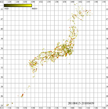
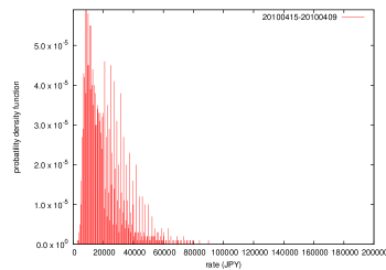
Figure 2: An example of rates distributions under the condition that two adults can stay at the hotel for one night at 15th April 2010 (Top). A probability density distribution of rates at 15th April 2010 (Bottom). This data have been sampled on 9th April 2010. Yellow (black) filled squares represent hotel plans cost 50,000 JPY (1,000) JPY per night. Red filled squares represent hotel plans cost over 50,000 JPY per night.

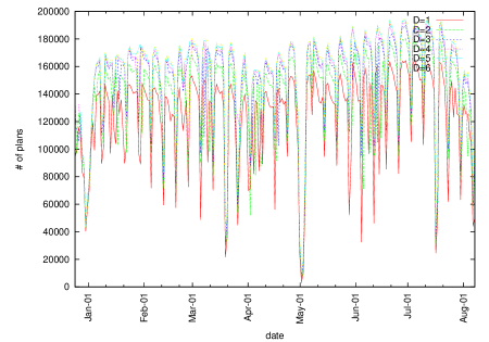
Figure 3: The number of hotels in which two adults can stay one night for a period from 24th Dec 2009 to 4th November 2010.

3 Overview of the data

The number of room opportunities in which two adults can stay is counted from the recorded csv files throughout the whole sampled period. Fig. 3 shows the daily number of room opportunities. From this graph, we found three facts:

(1)There exists weekly fluctuation for the number of available room opportunities.

(2)There is a strong dependence of the number of available opportunities on the Japanese calendar. Namely, Saturdays and holidays drove reservation activities of consumers. For example, during the New Year holidays (around 12/30-1/1) and holidays in the spring season (around 3/20), the time series of the numbers show big drops.

(3)The number eventually increases as the date of stay reaches. Specifically, it is observed that the number of opportunities drastically decreases two days before the date of stay.

Fig. 4 shows the number of available room opportunities at four regions for the period from 24th Dec 2009 to 4th November 2010. We calculated the numbers at 010502 (Otaru), 072005 (Aizu-Kohgen, Yunogami, and Minami-Aizu), 136812 (Shiragane), and 171408 (Yuzawa). It is found that there are regional dependences of their temporal development.

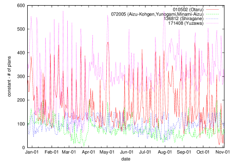
Figure 4: The number of demand for four region per day. It is found that there exists regional dependence of their fluctuations.

Furthermore, we show that dependence of averaged rates all over the Japan on calendar dates in Fig. 5. On the New Year holidays in 2010, it is confirmed that the averaged rates rapidly decrease, meanwhile, on the spring holidays in 2010 the averaged rates rapidly increase. This difference seems to arise from the difference of consumers motivation structure and preference on price levels between these holiday seasons.

Fig. 6 shows that the dependence of averaged rates at four regions on calendar dates. The tendency of averaged rates differs from each other. Specifically, the New Year holidays and the summer vacation season exhibit such difference. This means that demand-supply situations depend on regions. We need to know tendency of the demand-supply situations of each area in a rigorous manner.

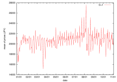
Figure 5: Time series of average rates of room opportunities on stay dates for four region. The mean value of rates is calculated from all the available room opportunities which are observed on each stay date.

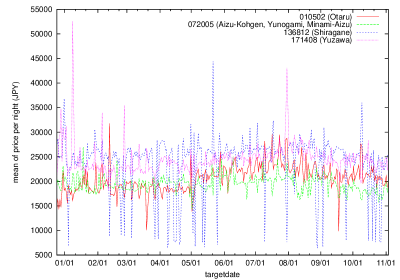
Figure 6: Time series of average rates of room opportunities on stay dates for four region. The mean value of rates is calculated from all the available room opportunities which are observed on each stay date.

4 Model

Let $N_{m}$ and $M$ be the total number of potential rooms at the area $m$ and the total number of potential consumers. The total number of opportunities $N_{m}$ may be assumed to be constant since the Internet booking style has been sufficiently accepted, and almost hotels offer their rooms via the Internet. Ignoring the birth-death process of consumers, we also assume that $M$ should be be constant.

We further assume that a Bernoulli random variable represents booking decision of a consumer from $N_{m}$ kinds of room opportunities. In order to express the status of rooms within the observation period (one day), we introduce $M$ Bernoulli random variables with time-dependent success probability $p_{m}(t)$,

$$y_{mi}(t)=\left\{\begin{array}[]{lll}1&w.p.\quad p_{m}(t)&\mbox{(the $i$-th consumer holds a reservation)}\\ 0&w.p.\quad 1-p_{m}(t)&\mbox{(the $i$-th consumer does not holds a reservation)}\\ \end{array}\right.,$$ (1)

where $y_{mi}(t)\quad(i=1,\ldots,M)$ represents the status of the $i$-th consumer for a room at time $t$.

If we assume that $p_{m}(t)$ is sufficiently small, so that $N_{m}>\sum_{i=1}^{M}y_{mi}(t)$, then the number of room opportunities at time $t$ may be proportional to the differences between the total number of potential rooms and the number of booked rooms at time $t$

$$Y_{m}(t)\propto N_{m}-\sum_{i=1}^{M}y_{mi}(t).$$ (2)

Namely, we have

$$Z_{m}(t)=kN_{m}-Y(t)=k\sum_{i=1}^{M}y_{mi}(t),$$ (3)

where $k$ is a positive constant.

Assuming further that $y_{1}(t),\ldots,y_{M}(t)$ are independently, identically, distributed, we obtain that the number of available opportunities $\sum_{i=1}^{M}y_{mi}(t)$ follows a binomial distribution $\mbox{B}(M,r_{m}(t))$. Furthermore, assuming $r_{m}\ll 1$, $M\gg 1$, $Mr_{m}\gg 1$, we can approximate the demand $Z_{m}(t)=kN_{m}-Y_{m}(t)$ as a Poisson random variable, which follows

$$\mbox{Pr}_{Z}(l=Z_{m}|r_{m}(t))=\frac{\{Mkp_{m}(t)\}^{l}}{l!}e^{-\{Mkp_{m}(t)\}}=\frac{\{Mr_{m}(t)\}^{l}}{l!}e^{-\{Mr_{m}(t)\}},$$ (4)

where we define $kp_{m}(t)$ as $r_{m}(t)$.

Since the agents have some interactions with one another, their psychological atmosphere (mood), which is collectively created by agents, influences their decision. Such a psychological effect may be expressed as probability fluctuations for success probability $r_{m}(t)$ at time $t$ in the Bernoulli random variable.

Let us assume that the time-dependent probability $r_{m}(t)\quad(0\leq r_{m}(t)\leq 1)$ is sampled from a probability density $F_{m}(r)$. From Eq. (4), the marginal distribution for the Poisson distribution conditioning on $r_{m}$ with probability fluctuation $F_{m}(r_{m})$ is given by

$$\mbox{Pr}_{Zm}(l=Z_{m})=\int_{0}^{1}F_{m}(r_{m})\frac{(Mr_{m})^{l}}{l!}e^{-Mr_{m}}dr_{m}.$$ (5)

Since we can observe the number of available opportunities $Z_{m}(t)$, we may estimate parameters of the distribution $F_{m}(r_{m})$ from the successive observations.

For the sake of simplicity, we further assume that $r_{m}(t)$ is sampled from discrete categories $r_{mi}$ with probability $a_{mi}$ ($0\leq r_{mi}\leq 1$; $i=1,\ldots,K_{m};\sum_{i=1}^{K_{m}}a_{mi}=1$). These parameters are expected to describe motivation structure of consumers depending on calendar days (weekdays/weekends and special holidays, business purpose/recreation and so forth). Then since $F_{m}(r_{m})$ is given by

$$F_{m}(r_{m})=\sum_{i=1}^{K_{m}}a_{mi}\delta(r_{m}-r_{mi}),$$ (6)

$\mbox{Pr}_{Zm}(l=Z_{m})$ is calculated as

$$\mbox{Pr}_{Zm}(l=Z_{m}) = \int_{0}^{1}F(r_{m})\frac{(Mr_{m})^{l}}{l!}e^{-Mr_{m}}dr_{m},$$ (7)

$$= \sum_{i=1}^{K_{m}}a_{mi}\frac{(Mr_{mi})^{l}}{l!}e^{-Mr_{mi}}.$$

Hence, Eq. (7) is concerned with a finite mixture of Poisson distributions.

5 Estimation procedure by means of the EM algorithm

The construction of estimators for finite mixtures of distributions has been considered in the literature of estimation. Estimation procedures for Poissonian mixture model have been successively studied by several researchers. Specifically moment estimators and maximum likelihood estimators are intensively studied.

The moment estimators were tried on a mixture of two normal distributions by Karl Peason as early as 1894. Graphical solutions have been given by Cassie (1954), Harding (1949) and Bhattacharya (1967). Rider discusses mixtures of binomial and mixtures of Poisson distributions in the case of two distributions (Rider, 1961).

Hasselblad proposed the maximum likelihood estimator and derived recursive equations for parameters (Hasselblad, 1969). The effectiveness of the maximum likelihood estimator for the mixtures of Poissonian distributions is widely recognized. Dempster discusses the EM-algorithm for mixtures of distributions in the several cases (Dempster, 1977). By using the EM-algorithm, we can obtain parameter estimates from mixing data.

Let $z_{m}(1),\ldots,z_{m}(T)$ be the number of demand (the number of potential room opportunities minus the number of available room opportunities) computed at each observation day. From the observation sequences, let us consider a method to estimate parameters of Eq. (7) based on the maximum likelihood method. In this case, since the log-likelihood function can be described as

$$L_{m}(a_{m1},\ldots,a_{mK_{m}},r_{m1},\ldots,r_{mK_{m}})=\sum_{s=1}^{T}\log\Bigl{(}\sum_{i=1}^{K_{m}}a_{mi}\frac{(Mr_{mi})^{z(s)}}{z(s)!}e^{-Mr_{mi}}\Bigr{)},$$ (8)

parameter estimates are obtained by the maximization of the log-likelihood function $L_{m}(a_{m1},\ldots,a_{mK_{m}},r_{m1}\ldots,r_{mK_{m}})$

$$\{\hat{a}_{m1},\ldots,\hat{a}_{mK},\hat{r}_{m1},\ldots,\hat{r}_{mK}\}=\underset{\{a_{mi}\},\{r_{mi}\}}{\mbox{arg max}}\quad L_{m}(a_{m1},\ldots,a_{mK_{m}},r_{m1}\ldots,r_{mK})$$ (9)

under the constraint $\sum_{i=1}^{K_{m}}a_{mi}=1$.

The maximum likelihood estimator for the mixture of Poisson models given by Eq. (9) can be derived by setting the partial differentiations of Eq. (8) with respect to each parameter as zero (See A). They lead to the following recursive equations for parameters;

$$a_{mi}^{(\nu+1)} = \frac{1}{T}\sum_{t=1}^{T}\frac{a_{mi}^{(\nu)}F_{mi}^{(\nu)}(z_{m}(t))}{G_{m}^{(\nu)}(z_{m}(t))}\quad(i=1,\ldots,K_{m}),$$ (10)

$$r_{mi}^{(\nu+1)} = \frac{1}{M}\frac{\sum_{t=1}^{T}z_{m}(t)\frac{F_{mi}^{(\nu)}(z_{m}(t))}{G_{m}^{(\nu)}(z_{m}(t))}}{\sum_{t=1}^{T}\frac{F_{mi}^{(\nu)}(z_{m}(t))}{G_{m}^{(\nu)}(z_{m}(t))}}\quad(i=1,\ldots,K_{m}),$$ (11)

where

$$F_{mi}^{(\nu)}(x) = \frac{(Mr_{mi}^{(\nu)})^{x}e^{-Mr_{mi}^{(\nu)}}}{x!},$$ (12)

$$G_{m}^{(\nu)}(x) = \sum_{i=1}^{K_{m}}a_{mi}^{(\nu)}F_{mi}^{(\nu)}(x).$$ (13)

These recursive equations give us a way to estimate parameters by starting from an adequate set of initial values. These recursive equations are also referred to as the EM-algorithm for the mixture of Poisson distributions (Dempster, 1977; Liu, 2006).

In order to determine the adequate number of parameters, we introduce the Akaike Information Criteria (AIC), which is defined as

$$AIC(K_{m})=4K_{m}-2\hat{L}_{m},$$ (14)

where $\hat{L}_{m}$ is the maximum value of the log-likelihood function in terms of $2K_{m}$ parameter estimates. $\hat{L}_{m}$ is computed from the log-likelihood value per observation with parameter estimates obtained from the EM-algorithm,

$$\hat{L}_{m}=\sum_{s=1}^{T}\log\Bigl{(}\sum_{i=1}^{K_{m}}\hat{a}_{mi}\frac{(M\hat{r}_{mi})^{z_{m}(s)}}{z_{m}(s)!}e^{-M\hat{r}_{mi}}\Bigr{)}.$$ (15)

Since it is known that the preferred model should be the one with the lowest AIC value, we obtain the adequate number of categories $K_{m}$ as

$$\hat{K_{m}}=\underset{K_{m}}{\mbox{arg min}}\quad AIC(K_{m}).$$ (16)

Furthermore, we consider the method to determine an underlying Poisson distribution from which the observation $z_{m}(s)$ was sampled. Since the underlying Poisson distribution is one of Poisson distributions for the mixture, its local likelihood function of $z_{m}(s)$ may be maximized over all the local likelihood functions of $z_{m}(s)$. Based on this idea we propose the following method.

Let $R_{mi}(z)\quad(i=1,\ldots,K_{m})$ be log-likelihood functions of the $i$-th category at area $m$ with parameter estimate $\hat{r}_{mi}$. From Eq. (7), it is defined as

$$R_{mi}(z)=z\log M+\log\hat{r}_{mi}-M\hat{r}_{mi}\ \log\Bigl{(}z!\Bigr{)}.$$ (17)

By finding the maximum log-likelihood value $R_{mi}(z(s))$ for $i=1,\ldots,K_{m}$, we can select the adequate distribution where $z_{m}(s)$ was extracted. Namely, the adequate category $\hat{i}_{s}$ for $z_{m}(s)$ should be given as

$$\hat{i}_{s}=\underset{i}{\mbox{arg max}}R_{i}(z_{m}(s)).$$ (18)

6 Numerical simulation

Before going into empirical analysis on actual data on room opportunities with the proposed parameter estimation method, we calculate parameter estimates for artificial data with it.

We generate the time series $z(s)\quad(s=1,\ldots,T)$ from a mixture of Poisson distributions, given by

$$\left\{\begin{array}[]{llll}r(t)&=&r_{i}\quad w.p.\quad a_{i}\\ z(t)&\sim&\mbox{Pr}(l=Z(t)|r(t))=\frac{(Mr(t))^{l}}{l!}e^{-Mr(t)}\end{array}\right..$$ (19)

where $K$ is the number of categories, $a_{i}$ represents the probability for the $i$-th category to appear $(i=1,\ldots,K;\sum_{i=1}^{K}a_{i}=1)$.

We set $K=12$ and $M=100,000,000$. Using parameters shown in Tab. 2, we generated the artificial data shown in Fig. 7. Next, we estimated parameters from $T(=200)$ observations without any prier knowledge on the parameters.

As shown in Fig. 8 (top) the AIC values with respect to $K$ take the minima at $\hat{K}=12$. In order to confirm adequacy of parameter estimates, we conduct Kolmogorov-Smirnov (KS) test between the artificial data and sequences of random numbers with parameter estimates.

Fig. 8 (bottom) shows KS statistic at each $K$. Since at $\hat{K}=12$ the KS statistic is computed as 0.327, which is less than 1.36, the null hypothesis that these time series are sampled from the same distribution is not rejected at 5% significance level. Tab. 3 shows parameter estimates.

Furthermore, we selected values of $r_{i}$ for each observation by means of the proposed method mentioned in Sec. 5. The parameter estimates can be computed as a function of time $t$.

However, we found differences between the parameter estimates and the true values. Especially, if the close true values of parameters were estimated as the same parameters. As a result, the number of categories is estimated as $\hat{K}=12$, which differs from the number of the true set of parameters as $K=12$.

After determining the underlying distribution for each observation, we further computed estimation errors between the parameter estimates and true parameters for each observation. As shown in Fig. 9, we confirmed that their estimation error, defined as $|\hat{r}_{i}(t)-r_{i}(t)|$ is less than $8.0\times 10^{-6}$, and that their relative error, defined as $|\hat{r}_{i}(t)-r_{i}(t)|/r_{i}(t)$, is less than 0.3 %. It is confirmed that the parameter estimates by using the EM-algorithm agree with true values of parameters for the artificial time series.

Hence, it is concluded that the discrimination errors between two close parameters do not play a critical role for the purpose of the parameter identification at each observation.

Figure 7: Examples of time series generated from the Poissonian mixture model for $K=12$ and $M=100,000,000$.

Figure 8: The value of AIC for artificial data is shown as a function in terms of the number of parameters $K$ (left). The lowest value of AIC is found as 3803.20 at $K=12$. The KS statistic between the artificial data and estimated ones at each $K$ (right).

Figure 9: Each Parameter estimate for an observation is shown as a function in terms of time (left). The relative error between the true parameter and the estimated one (right).

Table 2: Parameters of the Poissonian mixture model to generate artificial time series. The number of categories is set as $K=12$.

$r_{1}$	0.000025	$a_{1}$ 0.109726
$r_{2}$	0.000223	$a_{2}$ 0.070612
$r_{3}$	0.000280	$a_{3}$ 0.073355
$r_{4}$	0.000479	$a_{4}$ 0.077612
$r_{5}$	0.000613	$a_{5}$ 0.094848
$r_{6}$	0.000652	$a_{6}$ 0.073841
$r_{7}$	0.001219	$a_{7}$ 0.090867
$r_{8}$	0.001233	$a_{8}$ 0.062191
$r_{9}$	0.001295	$a_{9}$ 0.077662
$r_{10}$	0.001341	$a_{10}$ 0.102573
$r_{11}$	0.001412	$a_{11}$ 0.085892
$r_{12}$	0.001570	$a_{12}$ 0.080821

Table 3: Parameter estimates of the Poissonian mixture model by using the EM estimator (bottom). The number of categories was estimated as $\hat{K}=12$ and its AIC value is obtained as $AIC=3803.20$.

$r_{1}$	0.0000247783 $a_{1}$	0.0900000000
$r_{2}$	0.0002229207 $a_{2}$	0.0700000000
$r_{3}$	0.0002806173 $a_{3}$	0.0550000000
$r_{4}$	0.0004798446 $a_{4}$	0.0650000000
$r_{5}$	0.0006137419 $a_{5}$	0.0800000000
$r_{6}$	0.0006516237 $a_{6}$	0.0950000000
$r_{7}$	0.0012185180 $a_{7}$	0.1041702140
$r_{8}$	0.0012324086 $a_{8}$	0.0808297860
$r_{9}$	0.0012946718 $a_{9}$	0.0850000000
$r_{10}$	0.0013420367 $a_{10}$	0.1050000000
$r_{11}$	0.0014120537 $a_{11}$	0.0800000000
$r_{12}$	0.0015688622 $a_{12}$	0.0900000000

7 Empirical results and discussion

In this section, we apply the proposed method to estimating parameters for actual data. We estimate the parameters $a_{mi}$ and $r_{mi}$ from the numbers, which is shown in Fig. 4 at four regions with the log-likelihood functions given in Eq. (8).

Fig. 4 shows estimated time series of the demand from 24th Dec 2009 to 4th November 2010. In order to obtain this demand, we assume that $N_{m}=\max_{t}\{{Z_{m}(t)+10}\}$ and that $M$ is approximately equivalent to the total population of Japan, so that $M=1,000,000,000$.

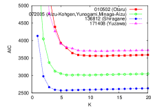
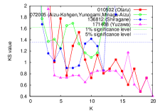
Figure 10: The value of AIC (left) and that of KS statistics (right) shown as a function in terms of the number of parameters $K$ for four areas.

According to the values of AIC as shown in Fig. 10 (left), the adequate number of parameters is estimated as $K=12$ (010502), $K=10$ (072005), $K=5$ (136812), and $K=11$ (171408), respectively. Fig. 10 (right) shows the KS value at each $K$. It is found that the KS test approves the mixture of Poisson distribution with parameter estimates in statistically significant. Tab. 4 shows the AIC and KS values at the adequate number of parameters for each area.

Table 4: At the adequate number of parameters, AIC, maximum log–likelihood ($ll$), KS value, and $p$-value for each region.

regional number	$K$	$AIC$	$ll$	$p$-value	KS value
010502	12	3558.31	1756.15	0.807	0.532
072005	10	3009.10	1485.55	0.187	1.088
136812	5	2572.33	1277.17	0.107	1.245
171408	11	3695.25	1826.62	0.465	0.850

Secondly, we confirmed that the relationship between mean of room rates and the number of opportunities (left) and that between existing probabilities $r_{mi}$ (right) for each day. Fig. 11 shows their scatter plots during the periods of 25th December 2009 and 4th November 2010. Each point represents their relation for each day. The variance of room rates proportional to the existence probability. It is confirmed that the mean of room rates for two adults per night is about 20,000 JPY. This means that the excess supply increases the uncertainty of room rates.

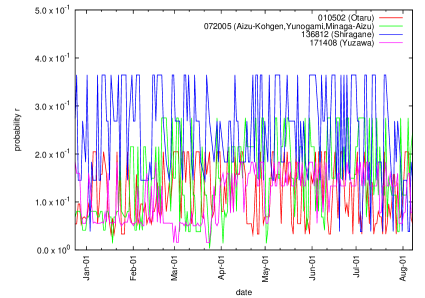
Figure 12: The parameter estimates from the number of available opportunities on observation date for four regions.

Thirdly, by means of the method to select the underlying distribution, from Poisson distributions for the mixture, we determined the category $i$ for each day. As shown in Fig. 12 (bottom), the probabilities show strong dependence on the Japanese calendar.

It is confirmed that there is both regional and temporal dependence of the probabilities. We found that the probabilities take higher values at each region on holidays and weekends (Saturday). It is observed that higher probabilities maintained in winter season at 072005 (Aizu-Kohgen,Yunogami,Minami-Aizu). This reason is because this place is one of winter ski resorts.

Specifically, on holidays and Saturdays, they take smaller values than on weekdays. Tabs. 5 and 6 show parameter estimates and exact dates included in each category at 010502 (Otaru), respectively. From this table we found that there is travel tendency of this region on seasons.

It is found that a lot of travelers visited and the hotel rooms were actively booked at this area on dates included in categories 1 to 3. On the other hand, this area were actively booked on dates included in categories 10 to 12.

The covariates among the numbers of room opportunities at different regions are the important factors to determine the demand-supply situations all over the Japan.

From Tab. 5, it is confirmed that in the case of Otaru the end of October to the beginning of November in 2010 was highly demanded season. This tendency is different from the calendar dates. The relationship between the number of opportunities and averaged rates is slightly different from that between the existence probability and the averaged rates. By using our proposed method we can compare the difference of comsumers’ demand between the dates. From the dependence of averaged prices on the probability $r_{i}$, we can understand preference and motivation structure of consumers for travel and tourism.

Table 5: Parameter estimates of the Poissonian mixture model by using the EM estimator. The number of categories were estimated as $\hat{K}=12$ at 010502.

$r_{1}$	0.0000001884	$a_{1}$	0.0195519998
$r_{2}$	0.0000005108	$a_{2}$	0.0245098292
$r_{3}$	0.0000008236	$a_{3}$	0.0548239374
$r_{4}$	0.0000010361	$a_{4}$	0.0332800534
$r_{5}$	0.0000010742	$a_{5}$	0.1572987311
$r_{6}$	0.0000012821	$a_{6}$	0.2045505810
$r_{7}$	0.0000015900	$a_{7}$	0.1402093740
$r_{8}$	0.0000019395	$a_{8}$	0.0801500614
$r_{9}$	0.0000023878	$a_{9}$	0.0959105486
$r_{10}$	0.0000027989	$a_{10}$	0.0544931969
$r_{11}$	0.0000032900	$a_{11}$	0.0661506482
$r_{12}$	0.0000041136	$a_{12}$	0.0690710390

Table 6: The dates included in each category for 010502 (Otaru).

1	2010-10-26,2010-10-27,201-10-28,2010-11-01,2010-11-03,2010-11-04
2	2010-09-01,2010-09-26,2010-09-30,2010-10-05,2010-10-18,2010-10-25,2010-10-31,2010-11-02
3	2010-02-01,2010-02-02,2010-02-03,2010-04-19,2010-04-21,2010-04-22,2010-05-12,2010-05-19,2010-05-23,2010-05-24,2010-05-25,2010-05-30,2010-07-14,2010-07-15,2010-07-15,2010-07-22,2010-07-31,2010-08-31,2010-09-06,2010-10-12,2010-10-12,2010-10-29
4	2010-01-11,2010-01-12,2010-01-15,2010-01-24,2010-02-04,2010-03-15,2010-03-23,2010-04-12,2010-04-13,2010-04-14,2010-04-18,2010-04-25,2010-05-09,2010-05-11,2010-05-13,2010-05-18,2010-05-26,2010-06-01,2010-06-03,2010-06-16,2010-06-30,2010-07-01,2010-07-06,2010-07-26,2010-07-27,2010-08-30,2010-09-15,2010-09-16,2010-09-20,2010-09-28,2010-10-04,2010-10-17,2010-10-21
5	2010-01-06,2010-01-07,2010-01-08,2010-01-13,2010-01-22,2010-01-29,2010-02-22,2010-03-01,2010-03-02,2010-03-03,2010-03-04,2010-03-07,2010-03-08,2010-03-10,2010-03-11,2010-03-16,2010-03-17,2010-03-18,2010-03-22,2010-03-25,2010-03-30,2010-03-31,2010-04-01,2010-04-06,2010-04-07,2010-04-11,2010-04-15,2010-04-16,2010-04-28,2010-05-06,2010-05-07,2010-05-14,2010-05-16,2010-05-22,2010-06-04,2010-06-06,2010-06-07,2010-06-08,2010-06-10,2010-06-11,2010-06-17,2010-06-21,2010-06-22,2010-07-02,2010-07-20,2010-08-03,2010-08-04,2010-08-05,2010-08-17,2010-08-20,2010-08-24,2010-09-07,2010-09-08,2010-09-12,2010-09-21,2010-09-22,2010-10-08,2010-10-20
6	2010-01-28,2010-01-30,2010-02-18,2010-02-26,2010-02-28,2010-03-05,2010-03-09,2010-03-12,2010-03-19,2010-03-29,2010-04-04,2010-04-09,2010-04-29,2010-05-05,2010-05-08,2010-05-15,2010-05-17,2010-05-21,2010-05-27,2010-06-02,2010-06-18,2010-06-20,2010-06-23,2010-06-27,2010-06-28,2010-07-09,2010-07-11,2010-07-12,2010-07-29,2010-08-02,2010-08-06,2010-08-19,2010-08-23,2010-08-29,2010-09-05,2010-09-17,2010-09-23,2010-09-27,2010-09-29,2010-10-01,2010-10-02,2010-10-19
7	2010-01-04,2010-01-16,2010-01-23,2010-02-09,2010-02-15,2010-02-16,2010-02-19,2010-02-21,2010-02-24,2010-03-14,2010-03-28,2010-04-02,2010-04-03,2010-04-10,2010-04-24,2010-06-09,2010-06-24,2010-07-04,2010-07-16,2010-08-22,2010-09-03,2010-09-10,2010-09-14,2010-09-24,2010-10-22,2010-10-30
8	2009-12-24,2010-12-27,2010-12-28,2010-01-03,2010-01-05,2010-01-10,2010-02-07,2010-02-08,2010-02-10,2010-02-17,2010-02-27,2010-03-26,2010-04-05,2010-04-08,2010-06-25,2010-07-08,2010-07-23,2010-07-25,2010-08-01,2010-08-11,2010-08-15,2010-08-16,2010-08-18,2010-08-21,2010-08-25,2010-10-07,2010-10-15,2010-10-16
9	2009-12-25,2009-12-26,2009-12-29,2010-01-09,2010-01-21,2010-02-05,2010-02-11,2010-02-14,2010-03-13,2010-04-20,2010-04-30,2010-07-03,2010-07-10,2010-08-08,2010-08-09,2010-08-10,2010-08-12,2010-08-26,2010-08-27
10	2009-12-30,2010-01-01,2010-01-02,2010-01-19,2010-02-12,2010-02-20,2010-03-06,2010-03-21,2010-05-29,2010-06-05,2010-06-12,2010-06-19,2010-07-30,2010-08-07,2010-08-13,2010-08-14,2010-09-04,2010-09-11,2010-10-11,2010-10-23
11	2009-12-31,2010-02-06,2010-02-13,2010-03-20,2010-03-27,2010-05-01,2010-05-02,2010-05-03,2010-05-04,2010-06-26,2010-07-17,2010-07-18,2010-07-24,2010-07-31,2010-08-28,2010-09-18,2010-09-19,2010-09-25,2010-10-09,2010-10-10
12	2010-01-18,2010-01-20,2010-01-25,2010-01-27,2010-04-23,2010-04-26,2010-04-27,2010-05-20,2010-05-28,2010-05-31,2010-06-13,2010-06-14,2010-06-29,2010-07-05,2010-07-13,2010-07-19,2010-07-21,2010-07-28,2010-09-02,2010-09-09,2010-09-13,2010-10-03,2010-10-13,2010-10-14,2010-10-24

Figure 11: The relationship between mean of rates per night and the number of opportunities and the relationship between it and existence probability for a period from 25th December 2009 to 4th Nov 2010 (left). Each point represents the relation on each observation day.

8 Conclusion

We analyzed the data of room opportunities collected from a Japanese hotel booking site. We found that there is strong dependence of the number of available opportunities on the Japanese calendar.

Firstly, We proposed a model of hotel booking activities based on a mixture of Poisson distributions with time-dependent intensity. From a binomial model with a time-dependent success probability, we derived the mixture of Poisson distributions. Based on the mixture model, we characterized the number of room opportunities at each day with different parameters regarding their difference as motivation structure of consumers dependent on the Japanese calendar.

Secondarily, we proposed a parameter estimation method on the basis of the EM-algorithm and a method to select the underlying distribution for each observation from Poisson distributions for the mixture through the maximization of the local log-likelihood value.

Thirdly, we computed parameters for artificial time series generated from the mixture of Poisson distributions with the proposed method, and confirmed that the parameter estimates agree with the true values of parameters in statistically significant. We conducted an empirical analysis on the room opportunity data. We confirmed that the relationship between the averaged prices and the probabilities of opportunities existing is associated with demand-supply situations. Furthermore, we extracted multiple time series of the numbers at four regions and found that the migration trends of travelers seem to depend on regions.

It was found that these large-scaled data on hotel opportunities enable us to see several invisible properties of travelers’ behavior in Japan.

As future work, we need to use more high-resolution data on booking of consumers at each hotel to capture demand-supply situations. If we can use such data, then we will be able to control room rates based on consumers’ preference. A future emerging technology will make it possible to see or foresee something which we can not see at this moment.

Appendix A Derivation of the EM-algorithm

In this section, we mention a derivation of the EM algorithm from the maximum likelihood estimation procedure. Let $G_{m}(z)$ represent a mixture of $K_{m}$ Poisson distributions $F_{mi}(z)$

$$F_{mi}(z) = \frac{(Mr_{mi})^{z}}{z!}e^{-Mr_{mi}},(i=1,\ldots,K_{m})$$ (20)

$$G_{m}(z) = \sum_{i=1}^{K_{m}}a_{mi}F_{mi}(z),$$ (21)

where $a_{mi}$ denote mixing ratios, which are normalized as

$$\sum_{i=1}^{K_{m}}a_{mi}=1.$$ (22)

From observations $\{z_{m}(t)\}$ the log-likelihood function in terms of the parameters $a_{mi},r_{mi}\quad(i=1,\ldots,K_{m})$ can be written as

$$L_{m}(a_{m1},\ldots,a_{mr},r_{m1},\ldots,r_{mK_{m}})=\sum_{t=1}^{T}\log G_{m}\bigl{(}z_{m}(t)\bigr{)}.$$ (23)

Inserting Eqs. (20) and (22) into Eq. (23), we have

$$L_{m}(a_{m1},\ldots,a_{mK_{m}},r_{m1},\ldots,r_{mK_{m}})=$$

$$\sum_{t=1}^{T}\log\Bigl{(}\sum_{i=1}^{K_{m}-1}a_{i}\frac{(Mr_{mi})^{z_{m}(t)}}{z_{m}(t)!}e^{-Mr_{mi}}+(1-\sum_{i=1}^{K_{m}-1}a_{mi})\frac{(Mr_{mK_{m}})^{z_{m}(t)}}{z_{m}(t)!}e^{-Mr_{mK}}\Bigr{)}.$$ (24)

Partially differentiating Eq. (24) in terms of $a_{mi}$ and $r_{mi}$, we obtain

$$\frac{\partial L_{m}}{\partial a_{mi}} = \sum_{t=1}^{T}\frac{F_{mi}(z(t))-F_{mK}(z_{m}(t))}{G_{m}(z_{m}(t))}\quad(i=1,\ldots,K_{m}-1),$$ (25)

$$\frac{\partial L_{m}}{\partial r_{mi}} = \sum_{t=1}^{T}\frac{a_{mi}F_{mi}(z_{m}(t))}{G_{m}(z_{m}(t))}\Bigl{(}\frac{z_{m}(t)}{r_{mi}}-M\Bigr{)}\quad(i=1,\ldots,K_{m}-1),$$ (26)

$$\frac{\partial L_{m}}{\partial r_{mK_{m}}} = \sum_{t=1}^{T}\frac{(1-\sum_{i=1}^{K_{m}}a_{mi})F_{K}(z_{m}(t))}{G_{m}(z_{m}(t))}\Bigl{(}\frac{z_{m}(t)}{r_{mK}}-M\Bigr{)}.$$ (27)

Multiplying $a_{mi}$ by Eq. (25) and summing them over $i$ we have

$$\sum_{t=1}^{T}\frac{F_{mi}(z_{m}(t))}{G_{m}(z_{m}(t))}=T\quad(i=1,\ldots,K_{m}),$$ (28)

and multiplying $a_{mi}/T$ by Eq. (28) we obtain

$$a_{mi}=\frac{1}{T}\sum_{t=1}^{T}\frac{a_{mi}F_{mi}(z_{m}(t))}{G_{m}(z_{m}(t))}\quad(i=1,\ldots,K_{m}).$$ (29)

From Eqs. (26) and (27) we immediately obtain

$$r_{mi}=\frac{1}{M}\frac{\sum_{t=1}^{T}z_{m}(t)\frac{F_{mi}(z_{m}(t))}{G_{m}(z_{m}(t))}}{\sum_{t=1}^{T}\frac{F_{mi}(z_{m}(t))}{G_{m}(z_{m}(t))}}\quad(i=1,\ldots,K_{m}).$$ (30)

Therefore, if we find an adequate set of initial values for parameters $\{a_{mi}^{\{0\}}\}$ and $\{r_{mi}^{\{0\}}\}$, then we can calculate parameters by using the update rule for $\{a_{mi}^{(\nu)}\}$ and $\{r_{mi}^{(\nu)}\}$

$$a_{mi}^{(\nu+1)} = \frac{1}{T}\sum_{t=1}^{T}\frac{a_{mi}^{({\nu})}F_{mi}^{(\nu)}(z_{m}(t))}{G_{m}^{(\nu)}(z_{m}(t))}\quad(i=1,\ldots,K_{m}),$$ (31)

$$r_{mi}^{(\nu+1)} = \frac{1}{M}\frac{\sum_{t=1}^{T}z_{m}(t)\frac{F_{mi}^{(\nu)}(z_{m}(t))}{G_{m}^{(\nu)}(z_{m}(t))}}{\sum_{t=1}^{T}\frac{F_{mi}^{(\nu)}(z_{m}(t))}{G_{m}^{(\nu)}(z_{m}(t))}}\quad(i=1,\ldots,K_{m}),$$ (32)

where

$$F_{mi}^{(\nu)}(z) = \frac{(Mr_{mi}^{(\nu)})^{z}}{z!}e^{-Mr_{mi}^{(\nu)}},$$ (33)

$$G_{m}^{(\nu)}(z) = \sum_{i=1}^{K_{m}}a_{mi}^{(\nu)}F_{mi}^{(\nu)}(z).$$ (34)

We compute these recursive equations by setting an arbitrary set of parameters. Some of them are convergent and the others divergent. Therefore, it is important for us to find an adequate set of initial values when we use the EM-algorithm given by Eqs. (31) and (32) for estimation. To do so, we use a way to find a candidate of parameters in a stochastic manner. This procedure consists of three parts.

The choice of initial values is based on Finch et al.’s algorithm Finch (1989). Their idea is that, given the mixing proportion $r_{mi}$, the $s$-th order statistics of observations $z_{m}(t_{s})\quad(s=1,\ldots,T)$ are separated into $K_{m}$ parts. Each sub-block contains the $i$-th $[a_{im}T]$ observations assumed to belong to the $i$-th component of the mixture. We compute mean of the $i$-th sub-block $\mu_{mi}$ and use it as initial value $r_{im}^{0}=\mu_{mi}/M$.

In the Monte Carlo step, we randomly allocate $r_{m1},\ldots,r_{mK_{m}}$, where $\sum_{i=1}^{K_{m}}r_{mi}=1$ and evaluate the log-likelihood function at the point. If the value of log-likelihood function at this point is finite, we choose this set of parameters as the new starting point for the recursive equation.

Further setting the set of parameters as an initial condition, we recursively calculate the EM-algorithm until the log-likelihood value converges. If it is greater than the maximum value of log-likelihood function which has already obtained in the Monte Carlo step, then the set of parameters as a candidate of parameter estimates.

Repeating this procedure until we can not find any points which improve the value of log-likelihood function in the Monte Carlo step, we estimate an adequate set of parameters. This algorithm is described as follows.

(0) Set $maxobj=0$ and $counter=0$.

(1) Generate normalized random numbers $a^{\prime}_{mi}$ as $a^{\prime}_{mi}=b^{\prime}_{mi}/\sqrt{\sum_{i=1}^{K_{m}}}b^{\prime}_{mi}$ by using i.i.d. uniform random numbers $b^{\prime}_{mi}$.

(2) $r_{mi}$ are generated with Finch et al.’s algorithm from $a^{\prime}_{im}$. If $counter>MAXCOUNT$, then go to Step (6).

(3) If $L_{m}(a^{\prime}_{m1},\ldots,a^{\prime}_{mK_{m}},r^{\prime}_{m1},\ldots,r^{\prime}_{mK})$ is greater than $maxobj$, then we set $maxobj$ as the value, $r_{mi}:=r^{\prime}_{mi}$ and $a_{mi}:=a^{\prime}_{mi}$, and go to Step (4). Otherwise go to Step (1).

(4) From the starting point $(a_{m1}\ldots,a_{mK},r_{m1},\ldots,r_{mK})$, compute Eqs. (10) and (11) recursively until the value of log-likelihood function converges.

(5) If the maximum value of log-likelihood function in terms of the converged set of parameters is larger than $maxobj$, then set the value as $maxobj$ and record the solution as a candidate of parameter estimates.

(6) $counter=counter+1$ and if $counter<MAXCOUNT$, then go to (1). Otherwise go to Step (7).

(7) Stop this computer program and display $maxobj$ and the recorded candidate as parameter estimates.

References

- Law (2009) R. Law, “Disintermediation of reservations”, International Journal of Contemporary Hospitality Management, 21 (2009) 766-772.
- Pilia (2008) R. Pilia, “Disintermediation of the hotel industry: the new perspects of online booking” available at : www.mymarking.net/agora/editoriali/contributi/dettaglio?articolo.asp?a=29&s=134&i=2584 (2008).
- Hagg & Weidlich (1984) G. Haag, and W. Weidlich, “A stochastic theory of interregional migration”, Geographical Analysis, 16 (1984) 331-357.
- Weidlich (2002) W. Weidlich, Sociodynamics: A Systematic Approach to Mathematical Modelling in the Social Sciences, Taylor and Francis, London (2002).
- Alfrano & Lux (2007) S. Alfrano and T. Lux, “A noise trader model as a generator of apparent financial power laws and long memory”, Macroeconomic Dynamics, 11 (2007) 80–101.
- Cassie (1954) R.M. Cassie, “Some uses of probability paper in the analysis of size frequency distributions”, Australian Journal of Marine and Freshwater Research, 5 (1954) 513–522.
- Harding (1949) J.P. Harding, “The use of probability paper of the graphical analysis of polymodal frequency distributions”, Journal of the Marine Biological Association, 28 (1949) 141–153.
- Bhattacharya (1967) C.G. Bhattacharya, “A simple method of resolution of a distribution into Gaussian components”, Biometrics, 23 (1967) 115-137.
- Rider (1961) R.P. Rider, “Estimating the parameters of mixed Poisson, binomial, and Weibull distributions by the method of moments”, Bulletin of the International Statistical Institute, 39 (1961) 225–232.
- Hasselblad (1969) V. Hasselblad, “Estimation of Finite Mixtures of Distributions from the Exponential Family”, Journal of the American Statistical Association, 64 (1969) 1459–1471.
- Dempster (1977) A.P. Dempster, N.M. Laird, and D.B. Rubin, “Maximum Likelihood from Incomplete Data via the EM Algorithm”, 39 (1977) 1–38.
- Liu (2006) Z. Liu, J. Almhana, V. Choulakian, R. McGorman, “Online EM algorithm for mixture with application to internet traffic modeling”, Computational Statistics and Data Analysis, 50 (2006) 1052–1071.
- Finch (1989) S. Finch, N. Mendell, H. Thode, “Probabilistic measures of adequacy of a numerical search for a global maximum”, Journal of American Statistical Association, 84 (1989) 1020-1023.