Statistics of resonances in one-dimensional disordered systems

Abstract

The paper is devoted to the problem of resonances in one-dimensional disordered systems. Some of the previous results are reviewed and a number of new ones is presented. These results pertain to different models (continuous as well as lattice) and various regimes of disorder and coupling strength. In particular, a close connection between resonances and the Wigner delay time is pointed out and used to obtain information on the resonance statistics.

I Introduction

The problem of resonances, also referred to as metastable or quasi-stationary states Landau-V3 , goes back to the early days of quantum mechanics Gamov-28 . A simple example of resonances Kumar-book is provided by a potential depicted in Fig. 1. There is a wall, $V=\infty$, for $x\geq L$ and a potential $V\left(x\right)=u\delta\left(x\right)$. For $u\rightarrow\infty$, a particle of mass $m$ has bound states at energies $\frac{1}{2m}\left(\frac{\pi\hbar n}{L}\right)^{2}$ [$n=1,2,\ldots$]. For any finite $u$ the spectrum becomes continuous. However, the strictly stationary states which existed at $u=\infty$ do leave a trace in the continuum and turn into resonances. They correspond to poles of the scattering matrix $S\left(E\right)$ on the unphysical sheet of the complex energy plane Landau-V3 ,Baz-book . An alternative, more direct approach to the problem of resonances amounts to solving the stationary Schrödinger equation with the boundary condition of an outgoing wave only Landau-V3 ,Gamov-28 . Thus for the potential in Fig. 1 one has to solve the equation

$$-\frac{d^{2}\psi}{dx^{2}}+\alpha\delta\left(x\right)\psi=\tilde{k}^{2}\psi\qquad\left(\alpha=\frac{2mu}{\hbar^{2}}\right)$$ (1)

with the boundary condition $\psi\left(x=L\right)=0$ and the outgoing wave condition $\psi\left(x\right)=e^{-i\tilde{k}x}$ for $x<0$. The latter condition makes the problem non-hermitian: the eigenvalues for $\tilde{k}$, and for the corresponding "energies" $\tilde{E}=\hbar^{2}\tilde{k}^{2}/2m$, will be generally complex.

The solutions of Eq. (1) is

$$\psi\left(x\right)=\left\{\begin{array}[]{ll}A\sin\tilde{k}(x-L),&0<x<L\\ e^{-i\tilde{k}x},&x<0\end{array}\right..$$ (2)

Matching the function and its derivative at $x=0$ results in

$$\left(1-i\gamma\tilde{k}L\right)\tan\tilde{k}L=-\gamma\tilde{k}L,$$ (3)

where $\gamma=\left(\alpha L\right)^{-1}\ll 1$. For $\gamma=0$ one recovers the bound states, $k_{n}L=\pi n$. For small $\gamma$ the solutions of (3) are obtained by iteration:

$$\tilde{k}_{n}L=\pi n\left(1-\gamma+\gamma^{2}\right)-i\left(\pi n\right)^{2}\gamma^{2}+O\left(\gamma^{3}\right).$$ (4)

One can immediately write down the "eigenenergies", $\tilde{E}_{n}=\hbar^{2}\tilde{k}_{n}^{2}/2m=E_{n}-\frac{i}{2}\Gamma_{n}$. The real part, $E_{n}$, gives the position of the resonance on the energy axis, whereas $\Gamma_{n}$ determines the resonance width. For $n$ not too large, namely, $n\ll\gamma^{-1}$, the resonances are sharp, i.e., their width is much smaller than their spacing on the energy axis. This simple example demonstrates how true bound states in a closed system ($u\rightarrow\infty$) turn into resonances, when the system is opened to the outside world (finite $u$, i.e. non-zero coupling constant $\gamma$).

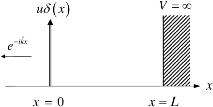
Figure 1: An illustration to the problem of resonances in a potential comprised of a $\delta$-function barrier and a hard wall.

Open quantum systems can be described in terms of an effective, non-Hermitian Hamiltonian whose complex eigenvalues give the position of the resonances in the complex energy plane (in addition, there might be real eigenvalues which correspond to the bound states). Such non-Hermitian Hamiltonians have been used for a long time in scattering theory, including scattering in disordered and chaotic systems Weidenmuller-69 ,Datta ,Dittes-00 ,Kottos . There is a considerable amount of work on resonances in disordered potentials Terraneo ,Pinheiro ,Titov-00 ,Weiss-06 ,Kottos-LDT-02 ,Kunz-Sh-06 ,Kunz-Sh-08 ,Feinberg ,Feinberg-09 . An example of one-dimensional random potential is depicted in Fig. 2. The potential $V\left(x\right)$ is zero for $x\leq 0$ and it is infinite for $x\geq L$. In the interval $0<x<L$, $V\left(x\right)$ is a random function of $x$, with zero mean and some well defined statistical properties. There is also a barrier $u\delta(x)$ at $x=0$ which allows to tune the coupling strength to the external world. For $u\rightarrow\infty$ (closed system) all states are localized within the system. Two such localized wave function are schematically shown in the figure: $\psi_{E}\left(x\right)$ is a state of positive energy, localized far away from the boundary $x=0$, i.e. its localization center $x_{0}$ is much larger than the localization length $\xi$. The function $\psi_{E^{\prime}}\left(x\right)$ corresponds to a negative energy state, which is localized essentially in a single deep potential well. When $u$ is made finite the localized state $\psi_{E}\left(x\right)$ will turn into a narrow resonance, with a width $\Gamma$ proportional to $\exp\left(-2x_{0}/\xi\right)$, while the state $\psi_{E^{\prime}}\left(x\right)$ will remain a true bound state. A theory of resonances in disordered chains should consider the statistical ensemble of all possible realizations of $V\left(x\right)$ and produce the probability distribution $P\left(\Gamma\right)$.

A quantity closely related to the resonance width is the Wigner delay time Wigner-55 ,Nussenzveig-02 which is a measure of the time spent by the particle in the scattering region and is defined as the energy derivative of the scattering phase shift. For the single-channel scattering, as presented in the setup (b) in Fig. 2, the solution of the scattering problem amounts to finding the phase $\theta\left(E\right)$ of the reflected wave, $e^{-ikx+i\theta\left(E\right)}$, due to the incident wave $e^{ikx}$. The corresponding Wigner delay time is defined as

$$\tau\left(E\right)=\hbar\frac{d\theta\left(E\right)}{dE}.$$ (5)

For a disordered system, $\theta\left(E\right)$ and $\tau\left(E\right)$ are random quantities, characterized by the joint distribution $P_{E,L}\left(\theta,\tau\right)$ over the ensemble of realizations. There exists a large body of work on the statistics of delay times for the scattering on disordered and chaotic systems Kumar-89 ,Kumar-00 ,Jayannavar-98 ,Osipov-Kot-00 ,Comtet-97 ,Comtet-99 ,Fyodorov-97 . In the presence of a sharp, well isolated resonance $\tilde{E}_{n}=E_{n}-\frac{i}{2}\Gamma_{n}$, delay time at the energy $E$ close to $E_{n}$ is given approximately by Nussenzveig-02

$$\tau\left(E\right)\approx\hbar\frac{\Gamma_{n}}{\left(E_{n}-E\right)^{2}+\Gamma_{n}^{2}/4},$$ (6)

which demonstrates the intimate relation between the resonance width and the delay time. Below (section IV) we obtain a relation between the delay time and the resonance width distributions which is exact in the limit of weak coupling to the lead, and which enables us to obtain information about resonances based on the existing knowledge of the delay time statistics.

Statistics of resonances and of delay times (or the closely related "dwell times") are of great interest in the physics of disordered media. For instance, in a disordered conductor the current carriers can be trapped for a long time, which lead to long tails in the decay of an electric current Mirlin-00 . Although our discussion is limited to "matter waves", obeying the Schrödinger equation, similar phenomena occur for electromagnetic waves as well. When a wave is injected into a random dielectric medium, it can spend there a very long time, before escaping from the sample. This phenomenon of long delay times has been extensively studied in experiments Genak-05 . Resonances and long escape times might be also relevant to the phenomenon of "random lasing", when an active random dielectric medium without any prefabricated cavities, exhibits lasing above some excitation threshold Cao-03 .

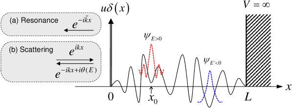
Figure 2: Schematic illustration of a 1D disordered system with one end ($x=L$) closed, and the other one ($x=0$) coupled to the lead through the $\delta$-function barrier. The resonance problem corresponds to (a): the outgoing wave condition is imposed and complex values of $\tilde{k}$ are found. The standard scattering problem is described in the set-up (b), where a particle with energy $E=\hbar^{2}k^{2}/2m$ is impinging on the system.

The organization of the paper is as follows. In section II we introduce a tight binding model and, following Kunz-Sh-06 ,Kunz-Sh-08 derive the effective non-Hermitian Hamiltonian for the resonance problem. Section III is devoted to the case when coupling between the disordered chain and the external lead is weak. Both the tight binding model and a random continuous potential are treated. In section IV a relation between the distributions of resonances and delay times is obtained, and used for studying properties of the resonances under various conditions (weak and strong coupling, finite and infinite chain). Section V specializes to the case of strong disorder, for the tight binding model, using the locator expansion technique.

II A tight binding model for resonances and its effective Hamiltonian

Along with the model of a continuous random potential, described in the Introduction, we also consider the tight binding (Anderson) model (TBM) depicted in Fig. 3. Black dotes, labeled by $n=1,2,...N$, designate sites in the chain. Each site is assigned a site energy $\epsilon_{n}$ chosen from some distribution $q(\epsilon)$. The energies on different sites are independent of each other. Open circles, labeled by $n=0,-1,-2,\ldots$, represent the perfect semi-infinite lead to which the chain is coupled. The lead simulates the free space outside the chain. All nearest neighbor sites of the chain are coupled to each other by a hopping amplitude $t$, and the same is true for all nearest neighbor sites of the lead. The only exception to this rule is the pair $n=\left(0,1\right)$ which provides coupling between the chain and the lead. The hopping amplitude for this pair is taken to be equal $t^{\prime}$. This allows us to tune the coupling from $t^{\prime}=0$ (closed chain) to $t^{\prime}=t$ (perfect coupling). The Schrödinger equation for the entire system (chain + lead) is a set of coupled equations:

$$-t\psi_{n+1}-t\psi_{n-1} =\tilde{E}\psi_{n}\quad\quad(n<0)$$ (7)

$$-t\psi_{-1}-t^{\prime}\psi_{1} =\tilde{E}\psi_{0}\quad\quad(n=0)$$ (8)

$$-t\psi_{2}-t^{\prime}\psi_{0}+\epsilon_{1}\psi_{1} =\tilde{E}\psi_{1}\quad\quad(n=1)$$ (9)

$$-t\psi_{n+1}-t\psi_{n-1}+\epsilon_{n}\psi_{n} =\tilde{E}\psi_{n}\quad\quad(1<n\leq N).$$ (10)

with the Dirichlet boundary condition $\psi_{N+1}=0$. Eqs. (7)-(10) are to be solved subjected to the boundary condition of an outgoing wave in the lead, i.e. $\psi_{n}\propto\exp(-i\tilde{k}n)$, for $n\leq 0$, with $\operatorname{Re}\tilde{k}>0$ (the wave propagates from right to left). The complex wave vector $\tilde{k}$ is related to $\tilde{E}$ by $\tilde{E}=-2t\cos\tilde{k}$. The complex solutions $\tilde{E}_{\alpha}=E_{\alpha}-\frac{i}{2}\Gamma_{\alpha}$ of Eqs. (7)-(10) yield the width of the resonances, as well as their position along the energy axes $E$.

As has been explained in the Introduction, the condition of an outgoing wave makes the problem a non-Hermitian one. In particular, for the tight binding model (Fig. 3) one can derive an explicit expression for an effective non-Hermitian Hamiltonian whose eigenvalues correspond to the resonances, in addition to the possible bound states. Using the plane wave solution $\psi_{n}\propto\exp(-i\tilde{k}n)$ in the lead $(n<1)$, it is straightforward to eliminate from Eqs. (7)-(10) all $\psi_{n}$’s with $n<1$ (for details see Datta ), thus reducing the problem to a system of equations for the amplitudes $\psi_{n}$ on the sites of the disordered chain alone ($n=1,2,...N$):

$$-t\psi_{n+1}-t\psi_{n-1}+\tilde{\epsilon}_{n}\psi_{n}=\tilde{E}\psi_{n}\quad\quad(n=1,2,\ldots,N)\,$$ (11)

with the boundary conditions $\psi_{0}=\psi_{N+1}=0$. Here $\tilde{\epsilon}_{n}=\epsilon_{n}$ for $n=2,3,....$, but not for $n=1$. This end site is assigned a complex energy

$$\tilde{\epsilon}_{1}=\epsilon_{1}-t\eta e^{i\tilde{k}},$$ (12)

where the parameter $\eta=\left(t^{\prime}/t\right)^{2}$ describes the coupling strength to the outside world. Thus, the effective non-Hermitian Hamiltonian $\tilde{H}$, defined in (11), differs from the Hermitian Hamiltonian, $H$, of the corresponding closed system (i.e., with $\eta=0$) only by the complex correction to the energy of the first site (the only site coupled directly to the lead), i.e.,

$$\tilde{H}=H-t\eta e^{i\tilde{k}}P,$$ (13)

where $P$ is the projection on site $n=1$. Note that the effective Hamiltonian $\tilde{H}$ depends, via $\tilde{k}$, on $\tilde{E}$. Therefore Eq. (11) does not constitute a standard eigenvalue problem and the eigenvalues of $\tilde{H}$ have to be determined self-consistently. We denote the complex variable $\tilde{E}\equiv z=E-\frac{i}{2}\Gamma$. It is shown in Kunz-Sh-08 that the resonances $z_{\alpha}$, in the complex $z$-plane, correspond to the roots (with $\operatorname{Im}z_{\alpha}<0$) of the equation

$$z-\epsilon_{1}-S_{1}(z)+\eta te^{i\tilde{k}(z)}=0,$$ (14)

where $S_{1}(z)$ is the self-energy for site $n=1$ and $\tilde{k}(z)$ is related to $z$ by $z=-2t\cos\tilde{k}$ (in Kunz-Sh-08 the variable $z$ was measured in units of $t$).

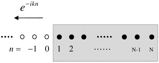
Figure 3: Resonance problem for one dimensional TBM.

III Treating the coupling term in $\tilde{H}$ as perturbation

When the coupling to the lead is weak ($\eta\ll 1$), the resonances can be obtained as small corrections to the eigenvalues of the closed system. For the tight binding effective Hamiltonian $\tilde{H}$, Eq. (13), first order perturbation theory with respect to the coupling term $-t\eta e^{i\tilde{k}}P$ gives

$$\tilde{E}_{\alpha}=e_{\alpha}-\eta t\psi_{\alpha}^{2}\left(1\right)e^{ik_{\alpha}}\equiv E_{\alpha}-\frac{i}{2}\Gamma_{\alpha},$$ (15)

where $e_{\alpha}$ is the energy of the unperturbed eigenstate $\psi_{\alpha}$ [the former notation $\psi_{n}$ has been changed into $\psi_{\alpha}\left(n\right)$ where subscript $\alpha$ labels the eigenstates], related to $k_{\alpha}$ by

$$e_{\alpha}=-2t\cos k_{\alpha}\Rightarrow e^{ik_{\alpha}}=-\frac{e_{\alpha}}{2t}+i\sqrt{1-\frac{e_{\alpha}^{2}}{4t^{2}}}.$$ (16)

Thus, the resonance width is

$$\Gamma_{\alpha}=2\eta\psi_{\alpha}^{2}\left(1\right)\sin k_{\alpha}=2\eta\psi_{\alpha}^{2}\left(1\right)\sqrt{t^{2}-\frac{1}{4}e_{\alpha}^{2}}.$$ (17)

In addition to the imaginary correction, $-i\Gamma/2$, there is also a real-valued correction, i.e. $E_{\alpha}=e_{\alpha}+\eta\psi_{\alpha}^{2}\left(1\right)e_{\alpha}/2$. This small energy shift on the real axis is of no interest. Note that the resonances exist only for $\left|e_{\alpha}\right|<2t$, i.e. within the band of the lead. For energies outside the band only bound states exist (real $\tilde{E}_{\alpha}$).

An expression analogous to (17) is obtained also for the continuous case depicted in Fig. 2, either as a continuum limit of (17) or by direct application of the perturbation theory. In the latter approach, matching the internal solution to the outgoing wave in the lead, one obtains

$$\frac{\psi\left(x=0^{+},\tilde{k}\right)}{\psi^{\prime}\left(x=0^{+},\tilde{k}\right)}=\frac{1}{i\tilde{k}-\frac{2mu}{\hbar^{2}}}.$$ (18)

Here $\psi\left(x,\tilde{k}\right)$ is the solution in the interval $0<x<L$ for the energy $E=\frac{\hbar^{2}\tilde{k}^{2}}{2m}$, which satisfies the closed-end boundary condition $\psi\left(x=L,\tilde{k}\right)=0$ plus the condition of the outgoing wave for $x\,<0$. For $u\rightarrow\infty$, Eq. (18) gives the spectrum and the eigenstates of the closed system, satisfying zero boundary condition $\psi_{\alpha}\left(0,k_{\alpha}\right)=0$. For weak coupling to the lead, $g\equiv\frac{2mu}{\hbar^{2}k_{\alpha}}\gg 1$, perturbative expansion of the above secular equation in powers of $g^{-1}$, yields

$$\Gamma_{\alpha}=4\frac{\hbar^{2}k_{\alpha}^{2}}{2m}\left[\frac{\hbar^{2}}{2mu}\right]^{2}\frac{\psi^{\prime}\left(0,k_{\alpha}\right)}{\psi_{k}\left(0,k_{\alpha}\right)},$$ (19)

where $\psi_{k}\left(x,k\right)=\frac{\partial}{\partial k}\psi\left(x,k\right)$. Then, employing the identity (see, e.g., Refs. Comtet-99 ,Nussenzveig-02 )

$$\left|\psi\right|^{2}=\frac{\hbar^{2}}{2m}\frac{d}{dx}\left(\frac{d\psi^{\ast}}{dx}\frac{d\psi}{dE}-\psi^{\ast}\frac{d^{2}\psi}{dxdE}\right),$$ (20)

the resonance width is expressed as

$$\Gamma_{\alpha}=\frac{\hbar^{2}k_{\alpha}}{2m}\left[\frac{\hbar^{2}k_{\alpha}}{mu}\right]^{2}\frac{\left|\psi_{\alpha}^{\prime}\left(0,k_{\alpha}\right)\right|^{2}}{2k_{\alpha}^{2}},$$ (21)

where $\psi_{\alpha}$ is the normalized to unity eigenfunction of the closed system with the eigenenergy $E_{\alpha}=\frac{\hbar^{2}k_{\alpha}^{2}}{2m}$. This expression is consistent with the exact effective Hamiltonian for the continuous open systems derived in Refs. Pichugin-01 ,Savin-03 .

Thus, both in the continuum and in TBM, for weak coupling to the lead there is one-to-one correspondence between the resonances and the eigenstates of the closed system, and the resonance width is related to the tail of the corresponding eigenstate at the boundary.

Certain simplifications occur in the limit of a semi-infinite chain. The TBM in the $N\rightarrow\infty$ limit has been studied in Kunz-Sh-08 , where the small-$\Gamma$ asymptotics for the density of resonances (DOR) has been rigorously derived in the weak coupling limit ($\eta\ll 1$). DOR in the $E,\Gamma$-plane, for a given realization of the disorder, is given by

$$\rho(E,\Gamma)=\sum_{\alpha}\delta(E-E_{\alpha})\delta(\Gamma-\Gamma_{\alpha}),$$ (22)

where $z_{\alpha}=E_{\alpha}-\frac{i}{2}\Gamma_{\alpha}$ are solutions of (14). For any $\Gamma\neq 0$, this expression for DOR has a well defined $N\rightarrow\infty$ limit and no division of the sum by $N$ is necessary, - in contrast to the usual case of the density of states (on the real axis) for a Hermitian problem. Note that the probability distribution of resonance width $P(\Gamma)$ (for some fixed $E$) does not have a well defined $N\rightarrow\infty$ limit and it approaches $\delta(\Gamma)$. (Indeed, for a semi-infinite chain an eigenstate will be localized, with probability $1$, at an infinite distance from the open end and, thus, will be ignorant about the coupling to the external world.) Thus, the appropriate quantity to look at for a semi-infinite chain is the DOR, rather than the probability distribution of resonance width. This subtle point is discussed in some detail in Kunz-Sh-06 .

Although the general considerations in Kunz-Sh-08 pertain to any coupling strength $\eta$, specific results for the average DOR where obtained only in the weak coupling limit, where the width of all resonances becomes proportional to $\eta$. The small-$\Gamma$ asymptotics for the average DOR $\left\langle\rho(E,\Gamma)\right\rangle$ is Kunz-Sh-08 (wherein the result is written in terms of some rescaled variables):

$$\left\langle\rho(E,\Gamma)\right\rangle={\frac{\nu\left(E\right)\xi\left(E\right)}{2\Gamma}},$$ (23)

where $\nu(E)$ and $\xi(E)$ are, respectively, the usual density of states (on the real energy axis) and the localization length for an infinite disordered chain. Angular brackets denote averaging over the ensemble of all random realizations. This asymptotic ($1/\Gamma$)- behavior is universal, in the sense that it holds for any degree of disorder and for any $-2t<E<2t$.

The $1/\Gamma$-asymptotics can be understood with the help of a simple intuitive argument which, in somewhat different versions, has appeared in Terraneo ,Pinheiro ,Titov-00 ,Weiss-06 ,Comtet-99 . The essence of the argument is that narrow resonances stem from states localized far away from the open boundary, say, at distance $x$. Such states will have an exponentially small tail at the boundary, proportional to $e^{-x/\xi}$, and the corresponding resonances will be exponentially narrow, $\Gamma\sim e^{-2x/\xi}$. The $1/\Gamma$- behavior then immediately follows from the assumption that the localization centers, $x$, are uniformly distributed in space.

One should keep in mind that, for a long but finite chain of $N$ sites, the $\left(1/\Gamma\right)$-tail will be cut off at very small $\Gamma$ of the order of $\exp\left(-2N/\xi\right)$. The extremely narrow resonances with $\Gamma\ll\exp\left(-2N/\xi\right)$ originate from states localized in the vicinity of the closed-end site $n=N$ and they should be treated separately (see below).

IV Relation between distributions of resonances and delay times

The rigorous asymptotic result of the previous section, Eq. (23), was obtained for a semi-infinite chain weakly coupled to an external lead. Things get more complicated if these restrictions are relaxed. In particular, the simple relation between the resonance width and the behavior of the corresponding eigenstate of the closed system [Eqs. (17) and (21)] breaks down when the coupling between the system and the lead becomes strong. In this section we discuss systems of finite size $L$ and beyond weak coupling limit.

In the Introduction we have mentioned the problem of the delay time $\tau\left(E,L\right)$ and the corresponding phase shift $\theta\left(E,L\right)$, for a particle of energy $E$ impinging on a random chain of length $L$. We designate by $P_{E,L}\left(\theta,\tau\right)$ the joint probability distribution of $\theta$ and $\tau$ for perfect coupling to the lead ($\eta=1$, or $u=0$) and relate this distribution to the average DOR $\left\langle\rho\left(E,\Gamma\right)\right\rangle$. Such relation is useful because it enables us to "transfer" the existing knowledge of the time delay in disordered chains Kumar-89 ,Kumar-00 ,Jayannavar-98 ,Osipov-Kot-00 ,Comtet-97 ,Comtet-99 into the field of resonances. To this end we introduce the quantity

$$\Phi_{\alpha}=\frac{1}{2}\left|\frac{\psi_{\alpha}^{\prime}\left(0\right)}{k}\right|^{2},$$ (24)

where $\psi_{\alpha}\left(x\right)$ is a normalized eigenfunction of the closed system satisfying the boundary conditions $\psi\left(0\right)=\psi\left(L\right)=0$. The average density of points $\left\{E_{\alpha},\Phi_{\alpha}\right\}$ in the $\left(E,\Phi\right)$-plane is

$$\left\langle\tilde{\rho}\left(E,\Phi\right)\right\rangle=\left\langle\sum_{\alpha}\delta\left(E-E_{\alpha}\right)\delta\left(\Phi-\Phi_{\alpha}\right)\right\rangle.$$ (25)

Although $\left\langle\tilde{\rho}\left(E,\Phi\right)\right\rangle$ is defined in terms of eigenvalues and eigenfunctions of the closed system, it can be related to the distribution $P_{E,L}\left(\theta,\tau\right)$ which describes scattering properties of the corresponding open system. The relation stems from the fact that for $\theta\left(E\right)=\pi$ the scattering wave function vanishes at $x=0$, so that the eigenvalues $E_{\alpha}$ are given by zeros of the function $\theta\left(E\right)-\pi$. This observation results in the identity

$$\delta\left(\theta\left(E\right)-\pi\right)=\sum_{\alpha}\left[\frac{d\theta\left(E\right)}{dE}\right]^{-1}\delta\left(E-E_{\alpha}\right)=\frac{\hbar}{\tau\left(E\right)}\sum_{\alpha}\delta\left(E-E_{\alpha}\right).$$ (26)

A generalization of this identity involves, in addition to the eigenvalues $E_{\alpha}$, also the eigenfunction-related quantity $\Phi_{\alpha}$, (24), and it reads Gurevich-PhD

$$\sum_{\alpha}\delta\left(E-E_{\alpha}\right)\delta\left(\Phi-\Phi_{\alpha}\right)=\frac{4}{\hbar v_{g}^{2}\Phi^{3}}\delta\left(\theta\left(E\right)-\pi\right)\delta\left(\tau\left(E\right)-\frac{2}{v_{g}\Phi}\right),$$ (27)

where $v_{g}=\hbar^{-1}\frac{dE}{dk}$ is the group velocity in the lead. This identity, upon averaging over the distribution $P_{E,L}\left(\theta,\tau\right)$ and using (25), yields the required relation between the quantities characterizing the open and the closed system:

$$\left\langle\tilde{\rho}\left(E,\Phi\right)\right\rangle=\frac{4}{\hbar v_{g}^{2}\Phi^{3}}P_{E,L}\left(\theta=\pi,\tau=\frac{2}{v_{g}\Phi}\right).$$ (28)

This expression holds for arbitrary $L$ and has a well defined $L\rightarrow\infty$ limit [cf. the discussion after Eq. (22)]. Let us note that Eq. (28) constitutes the strictly one-dimensional counterpart of the similar relations derived in Ref. Fyodorov-05 for the one-channel scattering from a higher-dimensional system. The results in Ref. Fyodorov-05  were obtained within the nonlinear sigma model and, thus, do not include the strictly 1D case discussed here.

Equations (24),(28) correspond to the continuous model. A completely similar treatment for the TBM yields precisely the same relation (28) [with $\hbar\equiv 1$], but with $\Phi_{\alpha}$ redefined as

$$\Phi_{\alpha}=\frac{\psi_{\alpha}^{2}\left(1\right)}{2\sin^{2}k},$$ (29)

and the group velocity in the lead given by $v_{g}=\frac{dE}{dk}=2t\sin k$.

The relation (28) is rather general. It holds for an arbitrary $L$, for any degree of disorder, and it is applicable to lattice models as well as to continuous ones. However, to employ this relation for the resonance statistics problem one more step is needed, namely, a relation between $\Phi_{\alpha}$ and $\Gamma_{\alpha}$. For the weak coupling case such a relation has been derived in the previous section for both the TBM [Eq. (17)] and the continuous potential (21). The two expressions can be unified into a single formula

$$\Gamma_{\alpha}=T\frac{\hbar v_{g}}{2}\Phi_{\alpha},\quad\left(T\ll 1\right)$$ (30)

where $T$ is the transmission coefficient through the potential barrier separating the lead from the chain. The latter is realized by a $\delta$-function potential in the continuum or by the weak hopping link $t^{\prime}$ in the TBM, as described previously, so that

$$T=\left[\begin{array}[]{ll}\frac{1}{1+\left(mu/\hbar^{2}k\right)^{2}},\vskip 3.0pt plus 1.0pt minus 1.0pt&\text{continuous model}\\ \frac{4\eta\sin^{2}k}{\left(1-\eta\right)^{2}+4\eta\sin^{2}k},&\text{TBM}\end{array}\right..$$ (31)

Note that the linear relation (30) between $\Gamma_{\alpha}$ and $\Phi_{\alpha}$ is valid only if $T$ is small (weak coupling). With the help of (30) one can map the density $\left\langle\tilde{\rho}\left(E,\Phi\right)\right\rangle$ in the $\left(E,\Phi\right)$-plane, Eq. (28), onto the average DOR in the $\left(E,\Gamma\right)$-plane:

$$\left\langle\rho\left(E,\Gamma\right)\right\rangle=\frac{\hbar T^{2}}{\Gamma^{3}}P_{E,L}\left(\theta=\pi,\tau=T\frac{\hbar}{\Gamma}\right).$$ (32)

This formula relates the average DOR to the delay time statistics. For a weak Gaussian white noise disorder and $L\gg\xi$ the distribution $P_{E,L}\left(\theta,\tau\right)$ does not depend on $\theta$ and has the following form Comtet-97 :

$$P_{E,L}\left(\theta,\tau\right)=\frac{\tau_{0}}{2\pi\tau^{2}}e^{-\tau_{0}/\tau}+\frac{1}{\pi^{2}\tau}e^{-\tau_{0}/2\tau}\int_{0}^{\infty}dse^{-L\left(1+s^{2}\right)/2\xi}\frac{s}{1+s^{2}}\sinh\frac{\pi s}{2}W_{1,is/2}\left(\frac{\tau_{0}}{\tau}\right),$$ (33)

where $\tau_{0}=\xi/v_{g}$ and $W_{1,is/2}$ is the Whittaker function (the same result is obtained for the weak correlated disorder Gurevich-PhD ). Expression (33), via (32), immediately yields the corresponding DOR.

In the limit $L/\xi\rightarrow\infty$, $\tau$ fixed, Eq. (33) reduces to

$$P_{E,\infty}\left(\theta,\tau\right)=\frac{1}{2\pi}\frac{\tau_{0}}{\tau^{2}}e^{-\tau_{0}/\tau},$$ (34)

so that

$$\left\langle\rho\left(E,\Gamma\right)\right\rangle=\frac{\nu_{0}\xi}{2\Gamma}e^{-\Gamma/\Gamma_{0}},$$ (35)

where $\nu_{0}=\left(\pi\hbar v_{g}\right)^{-1}$ is the density of states in the lead per unit length and

$$\Gamma_{0}=T\frac{v_{g}\hbar}{\xi}.$$ (36)

Eq. (35) coincides with the former result (23) for $\Gamma/\Gamma_{0}\ll 1$ and, in addition, gives an exponential suppression of the resonance density for $\Gamma/\Gamma_{0}>1$ (the exact density of states $\nu$ in (23) reduces to $\nu_{0}$ in the weak disorder limit).

For finite size chain ($L/\xi\approx 5$) and weak coupling ($T\approx.0004$) the distribution $P\left(\log\Gamma\right)=\left(\Gamma/\nu L\right)\left\langle\rho\left(E,\Gamma\right)\right\rangle$, calculated from (32),(33) is presented in Fig. 4 (solid line). For comparison, a numerical Monte-Carlo simulation was performed for the TBM at the energy close to the unperturbed band edge (dots in Fig. 4). The agreement is quite good. Let us discuss the example in Fig. 4 in more detail. First, the exponential factor $\exp\left[-\Gamma/\Gamma_{0}\right]$, which suppresses the large-$\Gamma$ probability, is present in both the semi-infinite, Eq. (35), and finite-$L$, Eq. (33), case. For $\Gamma$’s smaller than the characteristic value $\Gamma_{0}$, one can distinguish two regimes. In the intermediate regime, $e^{-2L/\xi}\ll\Gamma/\Gamma_{0}<1$, the behavior $P\left(\log\Gamma\right)\approx const$ [i.e. $\left\langle\rho\left(E,\Gamma\right)\right\rangle\sim 1/\Gamma$, Eq. (35)] is valid, since the opposite closed boundary of the system has not yet come into play. On the contrary, the regime of very narrow resonances, $\Gamma\ll\Gamma_{0}e^{-2L/\xi}$, is strongly affected by the boundary $x=L$. These resonances are associated with the eigenstates localized close to this boundary and are described by the nearly log-normal tail of the distribution.

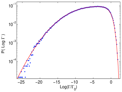
Figure 4: Weak coupling to the lead. The numerical simulation (dots) was done for the TBM (7)-(10) with $t=1$, $E=-1.9$, $\eta=0.001$ and system length $N=401$ sites. The uncorrelated disorder with a box distribution was implemented, which produced localization length $\xi=77.6$ sites. The analytical curve was calculated according to Eqs. (32) and (33).

Although the regime of the narrow resonances, $\Gamma\ll\Gamma_{0}e^{-2L/\xi}$ is contained in the analytical expressions (32),(33), it is worthwhile to give an independent, more direct derivation. Let us recall that the localization length $\xi$ is defined for an infinite system and, in this limit, it is a self-averaging quantity. In a long but finite size chain ($L\gg\xi$) the localizaton length, or more precisely its inverse (the Lyapunov exponent $\lambda$) is a fluctuating quantity with nearly a Gaussian distribution (see e.g. Comtet-99 and references therein)

$$P_{\lambda}\left(\lambda;L\right)=\sqrt{\frac{L\xi}{2\pi}}e^{-L\xi\left(\lambda-\xi^{-1}\right)^{2}/2}.$$ (37)

The tail of the extremely small $\Gamma$’s is related to the eigenstates localized near the closed end of the system, $x=L$, for which $\Phi_{\alpha}\approx\Phi_{0}e^{-2L\lambda}$, where the pre-factor $\Phi_{0}\sim\xi^{-1}$ is of minor importance. Then, neglecting the pre-exponential factor, the probability for $\Phi_{\alpha}\ll\Phi_{0}e^{-2L/\xi}$ decays like

$$P\left(\Phi\right)\propto\exp\left[-\frac{\left(\ln\left(\Phi/\Phi_{0}\right)+2L/\xi\right)^{2}}{8L/\xi}\right].$$ (38)

Using (30), one obtains the $\log$-normal cutoff of the DOR

$$\left\langle\rho\left(E,\Gamma\right)\right\rangle\propto\exp\left[-\frac{\left(\ln\left(\Gamma/\Gamma_{0}\right)+2L/\xi\right)^{2}}{8L/\xi}\right],\quad\frac{\Gamma}{\Gamma_{0}}\ll e^{-2L/\xi}$$ (39)

Similar cutoffs for the delay time and the average DOR have been derived in Refs. Comtet-99 and Titov-00 respectively.

So far the discussion was limited to the weak coupling case, when a simple relation between $\Phi_{\alpha}$ and $\Gamma_{\alpha}$ [Eq. (30)] could be rigorously derived. When the coupling parameter $T$ increases and approaches unity, the relation (30) ceases to be quantitatively accurate and turns into an order of magnitude estimate $\Gamma_{\alpha}\sim\hbar v_{g}\Phi_{\alpha}$. This relation is physically reasonable for narrow, isolated resonances. Such resonances stem from the eigenstates (of the closed system), which are localized far away from the open boundary $x=0$, and their width is much smaller than the mean level spacing. One can then trace a particular resonance, i.e. its width $\Gamma$ as a function of the increasing coupling strength $T$, without worrying about other resonances. It is therefore intuitively clear that the small-$T$ result, Eq. (30), can be qualitatively extrapolated up to the perfect coupling limit $T=1$.

One can support the above argument by a more elaborated analysis. Consider the formal solution of the one-channel scattering problem at energy $E$ close to a narrow isolated resonance $z_{r}=E_{r}-\frac{i}{2}\Gamma$. For small $E-E_{r}$, using general analytical properties of the scattering amplitude in the complex energy plane, the solution in the lead can be expanded as (see, e.g., Ref. Razavy )

$$\psi\left(x,E\right)=a\left(E-E_{r}+\frac{i}{2}\Gamma\right)e^{ikx}+a^{\ast}\left(E-E_{r}-\frac{i}{2}\Gamma\right)e^{-ikx},\quad x<0,$$ (40)

where, by identity (20), the complex constant $a$ satisfies (up to small corrections)

$$\left|a\right|^{2}=\frac{1}{\hbar v_{g}\Gamma}\int_{0}^{L}\left|\psi\left(x\right)\right|^{2}dx.$$ (41)

Energy $E_{\alpha}$ at which $\psi\left(x=0,E_{\alpha}\right)=0$ is the eigenenergy of the closed system, and by (40)

$$E_{\alpha}-E_{r}=\frac{\operatorname{Im}a}{2\operatorname{Re}a}\Gamma.$$ (42)

For the corresponding eigenfunction of the closed system, using (40),(41) in the definition (24), one obtains

$$\Phi_{\alpha}\approx\frac{\Gamma}{2\hbar v_{g}}\left[\left(\frac{\operatorname{Im}a}{\operatorname{Re}a}\right)^{2}+1\right]\geq\frac{\Gamma}{2\hbar v_{g}}.$$ (43)

Both (42) and (43) are meaningful as long as $\left(E_{\alpha}-E_{r}\right)\lesssim\Gamma$, i.e., $\left(\frac{\operatorname{Im}a}{\operatorname{Re}a}\right)^{2}\lesssim 1$, since otherwise the linear expansion (40) is not valid and higher orders should be included. With this reservation, Eq. (43) relates narrow isolated resonances to the well localized eigenstates of the closed system. However, contrary to (30), relation (43) is not deterministic, since it depends on the phase of $a$ (which is random for weak disorder). Replacing the unknown coefficient $\left[\left(\frac{\operatorname{Im}a}{\operatorname{Re}a}\right)^{2}+1\right]$ by a phenomenological constant $\beta^{-1}$ leads to

$$\Gamma_{\alpha}=2\beta\hbar v_{g}\Phi_{\alpha}.$$ (44)

With the relation (44) at hand, all the steps done for the weak coupling can be repeated, and Eqs. (32),(33) and (35) apply with the transmission coefficient $T$ replaced by $4\beta$ and the characteristic value $\Gamma_{0}$ [Eq. (36)] redefined as

$$\Gamma_{0}=4\beta\frac{v_{g}\hbar}{\xi}.$$ (45)

In the present case, however, the DOR obtained from Eqs. (32),(33) is valid only for $\Gamma\ll\Gamma_{0}$, since otherwise the isolated resonance approximation implied in the above argument is not applicable.

The above approximation was compared to the numerical simulation for the perfect coupling to the lead, Fig. 5. In both cases shown in Fig. 5, $L/\xi\approx\allowbreak 5$ and $L/\xi\approx\allowbreak 8$, the same fitting value $\beta\approx\allowbreak 0.68$ was used. As expected, a good agreement between the numerical simulation (dots) and the analytical result (solid line) is obtained only for $\Gamma<\Gamma_{0}$ (the deviation for the extremely small $\Gamma$’s is due to the numerical under-sampling).

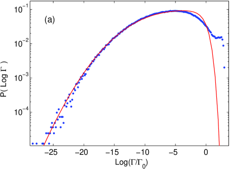
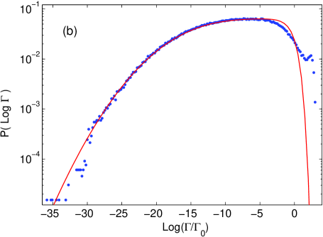
Figure 5: Resonance width distribution for the perfect coupling $T=1$. The analytical curve is calculcated according to Eqs. (32),(33) with $\Gamma_{0}$ given by (45). The numerical simulation was done as explained in Fig. 4, with the TBM parameters $t=1$, $E=-1.9$, $\eta=1$ and the uncorrelated disorder resulting in the localization length $\xi=77.6$ sites. The system length is (a) $N=401$ sites and (b) $N=601$ sites. The scatter of the numerical data for the extremely small values of $\Gamma/\Gamma_{0}$ occurs because of the insufficient numerical statistics.

V Strong Disorder

In this section we consider the case of strong disorder, when the hopping amplitude $t$ is much smaller than the characteristic width $W$ of the site energy distribution $q(\epsilon)$. For a semi-infinite chain the problem was considered in Kunz-Sh-06 , making use of a recursion relation for the self-energy. Here we employ the locator expansion, i.e. perturbation theory in $t$, which is the appropriate tool for strong disorder Anderson-58 ,Ziman . Our treatment is not restricted to a semi-infinite chain and, in particular, we address the question of the cutoff of the ($1/\Gamma$)-tail in a chain of large but finite $N$. Furthermore, no restriction on the coupling strength $\eta$ is imposed in our treatment.

For $t=0$ the Hamiltonian (13) corresponds to uncoupled sites and its eigenvalues coincide with the site energies $\epsilon_{j}$ ($j=1,2,....N$). When $t$ is switched on, some of these "unperturbed" eigenvalues acquire a complex correction, due to the last term in (13), and thus describe resonances. Our purpose is to find the imaginary part of this correction, in the leading order in $t$. (The small correction to the real part, $\epsilon_{j}$, introduces an unessential shift on the real axis of the complex energy plane and will be ignored). We designate the complex energy $\tilde{E}$ by $z=E-\frac{i}{2}\Gamma$ and look for the solutions, $z_{j}$, of Eq. (14), which we rewrite as

$$z-\tilde{\epsilon}_{1}-S_{1}(z)=0,$$ (46)

with

$$\tilde{\epsilon}_{1}=\epsilon_{1}-\eta te^{i\tilde{k}(z)}.$$ (47)

In order to see the mechanism by which the unperturbed solutions, $z_{j}^{(0)}=\epsilon_{j}$, acquire an imaginary correction, we employ the locator expansion for the self-energy $S_{1}(z)$. It can be represented diagrammatically as a sum over all paths which start at site $1$ and return to this site only once Anderson-58 ,Ziman . An example of such a path is drawn in Fig. 6. This path goes from site $1$ to $2$, proceeds from $2$ to $3$ and returns back to $1$ . This path contributes to $S_{1}$ a term $tg_{2}tg_{3}tg_{2}t$, where $g_{n}=(z-\epsilon_{n})^{-1}$ is the Green’s function (the locator) for an isolated site $n$. Thus, the general rule is that to a line connecting a pair of sites one assigns the number $t$, while to a site $n$ the corresponding locator is assigned. By inspecting Eq. (46) it becomes clear that an imaginary correction to the unperturbed solution $z_{j}^{(0)}$ is produced by paths, in the $S_{1}$ - expansion, which connect site $1$ to site $j$. Indeed, site $j$ has no direct knowledge about the connection to the outside world: this information must be transmitted to it from site $1$, via all intermediate sites. To leading order, it suffices to keep the shortest path. For site $3$ this is the path in Fig 6. Generalization to an arbitrary site $j$ is obvious and results in a path of $(j-1)$ loops which brings in a factor $t^{2(j-1)}$. This path produces the imaginary part of $z_{j}$, which is calculated from Eq.(46):

$$\operatorname{Im}z_{j}=t^{2(j-1)}\prod_{k=2}^{j-1}\frac{1}{(\epsilon_{j}-\epsilon_{k})^{2}}\operatorname{Im}\frac{1}{\epsilon_{j}-\tilde{\epsilon}_{1}}.$$ (48)

Since only the leading term (in powers of $t$) is kept, we have replaced in all the locators $z$ by $z_{j}^{(0)}=\epsilon_{j}$. For the same reason, $\tilde{k}(z)$ in the expression (47) can be replaced by $k(E)$. From the relation $E=-2t\cos k$ it follows that

$$\tilde{\epsilon}_{1}=\epsilon_{1}+t\eta\left(\frac{E}{2t}-i\sqrt{1-\frac{E^{2}}{4t^{2}}}\right).$$ (49)

Note that the imaginary part in (49) exists only for $|E|<2t$, i.e. only bound states in this energy interval (in a closed chain) turn into resonances upon coupling the chain to the lead (the same energy interval has already been identified in Sec. III). Eigenstates beyond this energy interval remain strictly bound states. Substituting (49) into (48) and, again, keeping only leading terms in $t$, one finally obtains:

$$-\operatorname{Im}z_{j}\equiv\frac{\Gamma_{j}}{2}=t^{2(j-1)}\eta\sqrt{t^{2}-\frac{E^{2}}{4}}\prod_{k=1}^{j-1}\frac{1}{\left(\epsilon_{j}-\epsilon_{k}\right)^{2}}.$$ (50)

The DOR in the $\left(E,\Gamma\right)$-plane is given by

$$\rho(E,\Gamma)=\sum_{j=2}^{N}\delta\left(E-\epsilon_{j}\right)\delta\left(\Gamma-\Gamma_{j}\right).$$ (51)

Since the small shift of the eigenvalues along the real axis is of no interest, we have set $E_{j}=\epsilon_{j}$ in Eq. (51). For a fixed $j$, resonance width $\Gamma_{j}$ depends on the energies of all previous sites, $k=1,2,\ldots,j-1$, but not on $\epsilon_{j}$. Therefore, the two $\delta$-functions in (51) are statistically independent, so that upon averaging

$$\left\langle\rho(E,\Gamma)\right\rangle=q\left(E\right)\left\langle\sum_{j=2}^{N}\delta\left(\Gamma-\Gamma_{j}\right)\right\rangle,$$ (52)

where, in the strong disorder limit, the site energy distribution function $q\left(E\right)$ coincides with the density of states per site in the closed system. To avoid cluttering the notation we set $E=0$ (middle of the band) and $\eta=1$ (perfect coupling). (Extension to arbitrary $E$ and $\eta$ requires some obvious minor modifications.)

Figure 6: Calculation of the self-energy in the locator expansion.

For this case

$$\left\langle\rho(E=0,\Gamma)\right\rangle=q\left(0\right)\sum_{j=2}^{N}\left\langle\delta\left(\Gamma-2t\prod_{k=1}^{j-1}\frac{t^{2}}{\epsilon_{k}^{2}}\right)\right\rangle.$$ (53)

It is convenient to define a random variable

$$A_{j}=\ln\prod_{k=1}^{j-1}\frac{t^{2}}{\epsilon_{k}^{2}}=-2\sum_{k=1}^{j-1}\ln\frac{\left|\epsilon_{k}\right|}{t}.$$ (54)

This is a sum of independent random variables with the average value $\left\langle\ln\frac{\left|\epsilon\right|}{t}\right\rangle=\int d\epsilon q\left(\epsilon\right)\ln\frac{\left|\epsilon\right|}{t}\equiv\alpha$ and variance $\left\langle\ln^{2}\frac{\left|\epsilon\right|}{t}\right\rangle-\alpha^{2}\equiv\beta$. For instance, for the Anderson model, when $\epsilon$ is uniformly distributed within a window $-\frac{tW}{2}<\epsilon<\frac{tW}{2}$, one has $\alpha=\left(\ln\frac{W}{2}-1\right)$ and $\beta=1$. Note that, in the strong disorder limit, $\alpha$ coincides with the inverse localization length (the Lyapunov exponent) Thouless-72 .

Since $N$ is a very large number, most of terms in (53) correspond to large $j$, so that $A_{j}$ has a Gaussian distribution, $P_{j}\left(A\right)$, with the average value $\left\langle A_{j}\right\rangle=-2\left(j-1\right)\alpha$ and variance $\left\langle\Delta A_{j}^{2}\right\rangle=4\beta j$, i.e.

$$P_{j}\left(A\right)=\frac{1}{\sqrt{8\pi\beta j}}\exp\left[-\frac{\left(A+2j\alpha\right)^{2}}{8j\beta}\right],$$ (55)

where $\left(j-1\right)$ was replaced by $j$. Eq. (53) then yields

$$\left\langle\rho(E=0,\Gamma)\right\rangle =q\left(0\right)\sum_{j=2}^{N}\int\delta\left(\Gamma-2te^{A}\right)P_{j}\left(A\right)dA$$

$$=\frac{q\left(0\right)}{\Gamma}\sum_{j=2}^{N}\frac{1}{\sqrt{8\pi\beta j}}\exp\left[-\frac{\left(\ln\left(\Gamma/2t\right)+2j/\xi\right)^{2}}{8j\beta}\right],$$ (56)

where $\xi=1/\alpha$ is the localization length in the middle of the band ($E=0$). The lower limit of summation, $j=2$, should not be taken literally and it is of no importance, since for small resonance width $\Gamma$ the sum is dominated by large-$j$ terms.

For narrow (but not too narrow) resonances, when $1\ll-\ln\left(\Gamma/2t\right)\ll N/\xi$, the sum is dominated by terms with $j$ near $j_{0}\approx-\left(\xi/2\right)\ln\left(\Gamma/2t\right)\gg 1$. Then, the sum in (56) can be approximated by an integral and

$$\left\langle\rho(E=0,\Gamma)\right\rangle\approx\frac{q\left(0\right)\xi\left(0\right)}{2\Gamma},$$ (57)

in agreement with the universal result in Eq. (23). This $1/\Gamma$ behavior is cut off sharply for very narrow resonances, such that $-\ln\left(\Gamma/2t\right)\gg N/\xi$. These resonances stem from states which are localized in the vicinity of the sample boundary at $j=N$. The sum (56) is then dominated by the last term, i.e.

$$\left\langle\rho(E=0,\Gamma)\right\rangle\approx\frac{q\left(0\right)}{\Gamma}\frac{1}{\sqrt{8\pi\beta N}}\exp\left[-\frac{\left(\ln\left(\Gamma/2t\right)+2N/\xi\right)^{2}}{8N\beta}\right],$$ (58)

i.e. for $-\ln\left(\Gamma/2t\right)>2N/\xi$ the DOR rapidly (faster than any power of $\Gamma$) approaches zero with decreasing $\Gamma$. This kind of $\log$-normal tails are well known in the theory of disordered electronic systems Mirlin-00 .

It is instructive to compare the strong disorder result, Eq. (58), with the expression (39) which was derived in the opposite case of weak disorder. The main difference between the two expressions, besides the fact that in (39) the pre-exponential factor has not been written down, is that the exponent in (39) contains the single parameter $L/\xi$, whereas (58) depends in addition on the parameter $\beta/\alpha$ [indeed, $8N\beta$ can be written as $8\left(N/\xi\right)\left(\beta/\alpha\right)$]. The parameter $\beta/\alpha$ is a non-universal number which depends, for instance, on the chosen distribution for the site energies, $q\left(\varepsilon\right)$. The same situation is well known to occur in the study of the transmission coefficient $T$ through a disordered chain of length $L$. The distribution of $\ln T$ is Gaussian. If the disorder is weak, then there is a universal relation between the mean and the variance of $\ln T$ (single parameter scaling). On the other hand, for strong disorder the two become independent of one another (two parameter scaling) Shapiro-88 .

VI Conclusion

Statistics of resonances in disordered one-dimensional chains is a formidable problem which does not easily lend itself to a rigorous analysis. In this paper we have reviewed some of the existing results and have extended them in various directions. We consider both a continuous random potential and the tight binding lattice model, and we tackle a variety of different cases, differing by size $L$ of the chain, by strength of the disorder or by coupling strength between the system and the external world. There is no efficient universal method for treating the problem in its full generality. Different techniques turn out to be appropriate in different regimes. In particular, we presented in some detail the method of locator expansion, most suitable for the strongly disordered lattice model. On the other hand, for weak disorder we were able to use some known rigorous results for the Wigner delay time problem to obtain information on resonance statistics.

BS is indebted to H. Kunz for previous collaboration on the subject. We acknowledge useful discussions with A. Comtet, J. Feinberg and C. Texier.

References

- (1) L.D. Landau and E.M. Lifshitz, Quantum mechanics: Non-Relativistic theory, Course of theoretical physics, vol. 3 (Pergamon, Oxford, 1977).
- (2) G. Gamov, Z. Phys. 51, 204 (1928).
- (3) see e.g. P.A. Mello and N. Kumar, Quantum transport in mesoscopic systems: complexity and statistical fluctuations, (Oxford University Press, Oxford, 2004).
- (4) A. I. Baz, A. Perelomov and I. B. Zeldovich, Scattering, Reactions and Decay in Nonrelativistic Quantum Mechanics, (Israel Program for Scientific Transactions, Jerusalem, 1969).
- (5) C. Mahaux and H.A. Weidenmüller, Shell-Model Approach to Nuclear Reactions (North-Holland, Amsterdam, 1969).
- (6) S. Datta, Electronic Transport in Mesoscopic Systems (Cambridge University Press, Cambridge, 1995).
- (7) F.M. Dittes, Phys. Rep. 339, 215 (2000).
- (8) T. Kottos, J. Phys. A 38, 10761 (2005), Special issue on trends in quantum chaotic scattering.
- (9) M. Terraneo and I. Guarnery, Eur. Phys. J. B 18, 303 (2000).
- (10) F.A. Pinheiro, M. Ruzek, A. Orlowski and B.A. van Tiggelen, Phys. Rev. E 69, 02605 (2004).
- (11) M. Titov and Y. V. Fyodorov, Phys. Rev. B 61, R2444 (2000).
- (12) M. Weiss, J.A. Nendez-Bermudes and T. Kottos, Phys. Rev. B 73, 045103 (2006).
- (13) T. Kottos and M. Weiss, Phys. Rev. Lett. 89, 56401 (2002).
- (14) H. Kunz and B. Shapiro, J. Phys. A 39, 10155 (2006).
- (15) H. Kunz and B. Shapiro, Phys. Rev. B 77, 054203 (2008).
- (16) J. Feinberg, Int. J. Theor. Phys. 50, 1116 (2011).
- (17) J. Feinberg, Pramana 73, 565 (2009).
- (18) E.P. Wigner, Phys. Rev. 98, 145 (1955).
- (19) C.A.A. de Carvalhoa, H.M. Nussenzveig, Phys. Rep. 364, 83 (2002).
- (20) A.M. Jayannavar, G.V. Vijayagovindan, N. Kumar, Z. Phys. B 75, 77(1989).
- (21) S.A. Ramakrishna and N. Kumar, Eur. Phys. J. B 23, 515 (2001).
- (22) S.K. Joshi and A.M. Jayannavar, Solid State Commun. 106, 363 (1999).
- (23) A. Ossipov, T. Kottos and T. Geisel, Phys. Rev. B 61, 11411 (2000).
- (24) A. Comtet and C. Texier, J. Phys. A: Math. Gen. 30 8017 (1997).
- (25) A. Comtet and C. Texier, Phys. Rev. Lett. 82, 4220 (1999).
- (26) Y. V. Fyodorov and H.-J. Sommers, J. Math. Phys. 38, 1918 (1997).
- (27) A.D. Mirlin, Phys. Rep. 326, 259 (2000).
- (28) For a review see A.Z. Genak and A.A. Chabanov, J. Phys. A 38, 10465 (2005), Special issue on trends in quantum chaotic scattering.
- (29) See a review by H. Cao in Waves in Random Media, 13, R1 (2003).
- (30) K. Pichugin, H. Schanz, and P. Šeba, Phys. Rev. E 64, 056227 (2001).
- (31) D.V. Savin, V.V. Sokolov, and H.-J. Sommers, Phys. Rev. E 67, 026215 (2003).
- (32) E. Gurevich, to be published elsewhere, PhD thesis, Technion, Haifa, Israel (2011).
- (33) A. Ossipov and Y. V. Fyodorov, Phys. Rev. B 71, 125133 (2005).
- (34) M. Razavy, Quantum theory of tunneling, (World Scientific Publishing Co., 2003).
- (35) P. W. Anderson, Phys. Rev. 109, 1492 (1958).
- (36) J.M. Ziman, Models of Disorder, (Cambridge University Press, Cambridge, 1979).
- (37) D. J. Thouless, J. Phys. C: Solid State Phys. 5, 77 (1972).
- (38) A. Cohen, Y. Roth and B. Shapiro, Phys. Rev. B 38, 12125 (1988).