Unification of multi-qubit polygamy inequalities

Abstract

We establish a unified view of polygamy of multi-qubit entanglement. We first introduce a two-parameter generalization of entanglement of assistance namely unified entanglement of assistance for bipartite quantum states, and provide an analytic lowerbound in two-qubit systems. We show a broad class of polygamy inequalities of multi-qubit entanglement in terms of unified entanglement of assistance that encapsulates all known multi-qubit polygamy inequalities as special cases. We further show that this class of polygamy inequalities can be improved into tighter inequalities for three-qubit systems.

I Introduction

As a quantum correlation among different systems, quantum entanglement shows an essential difference from classical correlations. If a pair of parties in a multi-party quantum system are maximally entangled then they cannot share any entanglement ckw ; ov nor classical correlations kw with the rest of the system. This restricted shareability of entanglement in multi-party quantum systems is known as monogamy of entanglement (MoE) T04 ; more entanglement shared between two parties necessarily implies less entanglement shared with the rest of the system. Furthermore, shared entanglement between two parties even limits the amount of classical correlation that can be shared with the other parties.

MoE plays a crucial role in many quantum information processing tasks. In quantum key-distribution protocols, the possible amount of information an eavesdropper could obtain about the secret key can be restricted by MoE, which is the fundamental concept of security proof. MoE also plays an important role in condensed-matter physics such as the $N$-representability problem for fermions anti .

The first characterization of MoE was proposed as an inequality in three-qubit systems ckw using concurrence ww to quantify shared bipartite entanglement. Later, monogamy inequality was generalized into multi-qubit systems in terms of various entanglement measures ov ; KSRenyi ; KT ; KSU , and also some cases of higher-dimensional quantum systems rather than qubits kds .

Whereas, monogamy inequality is about the restricted shareability of multipartite entanglement, the dual concept of the sharable entanglement, namely distributed entanglement, is known to have a polygamous property in multipartite quantum systems. A mathematical characterization for the polygamy of entanglement was first provided for multi-qubit systems gbs using concurrence of assistance (CoA) lve to quantify the distributed bipartite entanglement. Recently, a broad class of polygamy inequalities for multi-qubit systems was proposed KT , and a polygamy inequality in tripartite quantum systems of arbitrary dimension was also shown using entanglement of assistance (EoA) BGK .

Here, we provide a unified view of these polygamy inequalities of multi-qubit entanglement. We first introduce a two-parameter generalization of EoA namely unified entanglement of assistance (UEoA) for bipartite quantum states, and provide an analytic lower bound for UEoA in two-qubit systems. By investigating the functional relation between UEoA and concurrence, we establish a two-parameter class of polygamy inequalities of multi-qubit entanglement in terms of UEoA. This new class of polygamy inequalities reduces to every known multi-qubit polygamy inequalities as special cases, therefore our new class of polygamy inequalities also provides an interpolation among various polygamy inequalities of multi-qubit entanglement. We further show that our polygamy inequality can be improved into a tighter inequality for three-qubit pure states.

This paper is organized as follows. In Section II.1, we define UEoA for bipartite quantum states, and discuss its relation with CoA, EoA, and Tsallis entanglement of assistance (TEoA). In Section II.2, we provide an analytic lower bound of UEoA in two-qubit systems. In Section III, we derive a class of polygamy inequalities of multi-qubit entanglement in terms of UEoA, and summarize our results in Section IV.

II Unified Entanglement and Unified Entanglement of Assistance

II.1 Definition

Let us first recall the definition of unified entropy for quantum states ue1 ; ue2 . For $q,~{}s\geq 0$ such that $q\neq 1$, $s\neq 0$, unified-$(q,s)$ entropy of a quantum state $\rho$ is

$$S_{q,s}(\rho):=\frac{1}{(1-q)s}\left[{\left(\mbox{$\mathrm{tr}$}\rho^{q}\right)}^{s}-1\right].$$ (1)

Unified-$(q,s)$ entropy has singularities at $q=1$ or $s=0$, however it converges to von Neumann entropy as $q$ tends to 1;

$$\lim_{q\rightarrow 1}S_{q,s}(\rho)=-\mbox{$\mathrm{tr}$}\rho\log\rho=:S(\rho),$$ (2)

and Rényi-$q$ entropy renyi ; horo as $s$ tends to $0$,

$$\lim_{s\rightarrow 0}S_{q,s}(\rho)=\frac{1}{1-q}\log\mbox{$\mathrm{tr}$}\rho^{q}=:R_{q}(\rho).$$ (3)

For this reason, we can consider unified-$(q,s)$ entropy as von Neumann entropy or Rényi-$q$ entropy when $q=1$ or $s=0$ respectively; for any quantum state $\rho$ we just denote $S_{1,s}(\rho)=S(\rho)$ and $S_{q,0}(\rho)=R_{q}(\rho)$. We also note that unified-$(q,s)$ entropy converges to Tsallis-$q$ entropy  tsallis when $s$ tends to $1$,

$$S_{q,1}(\rho)=\frac{1}{1-q}\left(\mbox{$\mathrm{tr}$}\rho^{q}-1\right)=:T_{q}(\rho).$$ (4)

For a bipartite pure state ${\left|\psi\right\rangle}_{AB}$ and each $q,~{}s\geq 0$, its unified-$(q,s)$ entanglement KSU is defined as

$$E_{q,s}\left({\left|\psi\right\rangle}_{AB}\right):=S_{q,s}(\rho_{A}),$$ (5)

where $\rho_{A}=\mbox{$\mathrm{tr}$}_{B}{\left|\psi\right\rangle}_{AB}{\left\langle\psi\right|}$ is the reduced density matrix of ${\left|\psi\right\rangle}_{AB}$ onto subsystem $A$. For a mixed state $\rho_{AB}$, its unified-$(q,s)$ entanglement is

$$E_{q,s}\left(\rho_{AB}\right):=\min\sum_{i}p_{i}E_{q,s}({\left|\psi_{i}\right\rangle}_{AB}),$$ (6)

where the minimum is taken over all possible pure state decompositions of $\rho_{AB}=\sum_{i}p_{i}{\left|\psi_{i}\right\rangle}_{AB}{\left\langle\psi_{i}\right|}$.

Due to the continuity of unified-$(q,s)$ entropy with respect to $q$ and $s$, unified-$(q,s)$ entanglement in Eq. (6) converges to the entanglement of formation (EoF) as $q$ tends to 1,

$$\lim_{q\rightarrow 1}E_{q,s}\left(\rho_{AB}\right)=E_{\rm f}\left(\rho_{AB}\right),$$ (7)

where $E_{\rm f}(\rho_{AB})$ is EoF of $\rho_{AB}$ defined as

$$E_{\rm f}(\rho_{AB})=\min\sum_{i}p_{i}S(\rho^{i}_{A})$$ (8)

with $\mbox{$\mathrm{tr}$}_{B}|\psi^{i}\rangle_{AB}\langle\psi^{i}|=\rho^{i}_{A}$ and the minimization being taken over all possible pure state decompositions of $\rho_{AB}=\sum_{i}p_{i}{\left|\psi_{i}\right\rangle}_{AB}{\left\langle\psi_{i}\right|}$. When $s$ tends to $0$, unified-$(q,s)$ entanglement reduces to a one-parameter class of entanglement measures namely Rényi-$q$ entanglement KSRenyi

$$\lim_{s\rightarrow 0}E_{q,s}\left(\rho_{AB}\right)={\mathcal{R}}_{q}\left(\rho_{AB}\right).$$ (9)

Unified-$(q,s)$ entanglement also reduces to another one-parameter class called Tsallis-$q$ entanglement KT as $s$ tends to $1$,

$$\lim_{s\rightarrow 1}E_{q,s}\left(\rho_{AB}\right)={\mathcal{T}}_{q}\left(\rho_{AB}\right).$$ (10)

In other words, unified-$(q,s)$ entanglement is a two-parameter generalization of EoF including the classes of Rényi and Tsallis entanglement as special cases.

As a dual concept of EoF, EoA of a bipartite mixed state $\rho_{AB}$ is defined as cohen

$$E^{a}(\rho_{AB})=\max\sum_{i}p_{i}S(\rho^{i}_{A}),$$ (11)

where the maximum is taken over all possible pure state decompositions of $\rho_{AB}=\sum_{i}p_{i}|\psi^{i}\rangle_{AB}\langle\psi^{i}|$ with $\mbox{$\mathrm{tr}$}_{B}|\psi^{i}\rangle_{AB}\langle\psi^{i}|=\rho^{i}_{A}$. Here, we note that EoA in Eq. (11) is clearly a mathematical dual to EoF in Eq. (8) because one is the maximum average entanglement over all possible pure state decompositions whereas the other takes the minimum. Moreover, by introducing a third party $C$ that has the purification of $\rho_{AB}$, $E^{a}(\rho_{AB})$ can also be considered as the maximum achievable entanglement between $A$ and $B$ assisted by $C$ BGK . (This is the reason why it is called the assistance.) In other words, $E^{a}(\rho_{AB})$ is the maximal entanglement that can be distributed between $A$ and $B$ assisted by the environment $C$; therefore, EoA is also physically dual to the concept of formation.

Similar to the duality between EoF and EoA, we define UEoA of $\rho_{AB}$ as the maximum average entanglement

$$E_{q,s}\left(\rho_{AB}\right):=\max\sum_{i}p_{i}E_{q,s}({\left|\psi_{i}\right\rangle}_{AB})$$ (12)

over all possible pure state decompositions of $\rho_{AB}$. Due to the continuity of unified entropy with respect to $q$ and $s$, we have

$$\lim_{q\rightarrow 1}{E^{a}_{q,s}}\left(\rho_{AB}\right)=E^{a}\left(\rho_{AB}\right),$$ (13)

where $E^{a}(\rho_{AB})$ is the EoA of $\rho_{AB}$ in Eq. (11). When $q$ tends to $1$ UEoA reduces to TEoA KT ,

$$\lim_{s\rightarrow 1}E^{a}_{q,s}\left(\rho_{AB}\right)={\mathcal{T}}^{a}_{q}\left(\rho_{AB}\right),$$

where ${\mathcal{T}}^{a}_{q}\left(\rho_{AB}\right)$ is TEoA of $\rho_{AB}$ defined as

$${\mathcal{T}}^{a}_{q}\left(\rho_{AB}\right):=\max\sum_{i}p_{i}{\mathcal{T}}_{q}({\left|\psi_{i}\right\rangle}_{AB}).$$ (15)

II.2 Analytic Evaluation

For a bipartite pure state ${\left|\psi\right\rangle}_{AB}$, its concurrence ww , $\mathcal{C}({\left|\psi\right\rangle}_{AB})$ is

$$\mathcal{C}({\left|\psi\right\rangle}_{AB})=\sqrt{2(1-\mbox{$\mathrm{tr}$}\rho^{2}_{A})},$$ (16)

where $\rho_{A}=\mbox{$\mathrm{tr}$}_{B}({\left|\psi\right\rangle}_{AB}{\left\langle\psi\right|})$. For a mixed state $\rho_{AB}$, its concurrence is

$$\mathcal{C}(\rho_{AB})=\min\sum_{k}p_{k}\mathcal{C}({{\left|\psi_{k}\right\rangle}}_{AB}),$$ (17)

where the minimum is taken over all possible pure state decompositions, $\rho_{AB}=\sum_{k}p_{k}{{\left|\psi_{k}\right\rangle}}_{AB}{\left\langle\psi_{k}\right|}$.

For a two-qubit pure state ${\left|\psi\right\rangle}_{AB}$ with Schmidt decomposition

$${\left|\psi\right\rangle}_{AB}=\sqrt{\lambda_{0}}{\left|00\right\rangle}_{AB}+\sqrt{\lambda_{1}}{\left|11\right\rangle}_{AB}$$ (18)

with $\rho_{A}=\mbox{$\mathrm{tr}$}_{B}({\left|\psi\right\rangle}_{AB}{\left\langle\psi\right|})=\lambda_{0}{\left|0\right\rangle}_{A}{\left\langle 0\right|}+\lambda_{1}{\left|1\right\rangle}_{A}{\left\langle 1\right|}$, $\mathcal{C}({\left|\psi\right\rangle}_{AB})$ in Eq. (16) can be rewritten as

$$\mathcal{C}({\left|\psi\right\rangle}_{AB})=\sqrt{2(1-\mbox{$\mathrm{tr}$}\rho^{2}_{A})}=2\sqrt{\lambda_{0}\lambda_{1}},$$ (19)

Here we note that

$$2\sqrt{\lambda_{0}\lambda_{1}}=\left(\mbox{$\mathrm{tr}$}\sqrt{\rho_{A}}\right)^{2}-1=S_{\frac{1}{2},2}\left(\rho_{A}\right)=E_{\frac{1}{2},2}\left({\left|\psi\right\rangle}_{AB}\right),$$ (20)

therefore unified-$(q,s)$ entanglement of a two-qubit pure state ${\left|\psi\right\rangle}_{AB}$ reduces to the concurrence when $q=1/2$ and $s=2$. Consequently, we have

$$\mathcal{C}(\rho_{AB})=E_{\frac{1}{2},2}\left(\rho_{AB}\right),$$ (21)

for a two-qubit mixed state $\rho_{AB}$ because both concurrence and unified-$(q,s)$ entanglement of bipartite mixed states are defined by the minimum average entanglement over all possible pure-state decompositions of $\rho_{AB}$.

In two-qubit systems, concurrence has an analytic formula ww ; for a two-qubit state $\rho_{AB}$,

$$\mathcal{C}(\rho_{AB})=\max\{0,\lambda_{1}-\lambda_{2}-\lambda_{3}-\lambda_{4}\},$$ (22)

where $\lambda_{i}$’s are the eigenvalues, in decreasing order, of $\sqrt{\sqrt{\rho_{AB}}\tilde{\rho}_{AB}\sqrt{\rho_{AB}}}$ and $\tilde{\rho}_{AB}=\sigma_{y}\otimes\sigma_{y}\rho^{*}_{AB}\sigma_{y}\otimes\sigma_{y}$ with the Pauli operator $\sigma_{y}$. Moreover, concurrence in two-qubit systems is related with EoF by a monotonically increasing, convex function,

$$E_{\rm f}(\rho_{AB})={\mathcal{E}}(\mathcal{C}\left(\rho_{AB}\right)),$$ (23)

where

$${\mathcal{E}}(x)=H\left(\frac{1-\sqrt{1-x^{2}}}{2}\right),\hskip 14.22636pt\mbox{for }0\leq x\leq 1,$$ (24)

with the binary entropy function $H(t)=-[t\log t+(1-t)\log(1-t)]$ ww . This function relation between concurrence and EoF is also true for any bipartite pure state with Schmidt-rank 2. In other words, the analytic formula of concurrence in Eq. (22) together with the functional relation in Eq. (23) lead to an analytic formula of EoF in two-qubit systems.

Recently, it was shown that concurrence also has a functional relation with unified-(q,s) entanglement in two-qubit systems KSU ; for any two-qubit mixed state $\rho_{AB}$ (as well as any bipartite pure state with Schmidt-rank 2),

$$E_{q,s}\left(\rho_{AB}\right)=f_{q,s}\left(\mathcal{C}(\rho_{AB})\right),$$ (25)

for $q\geq 1$, $0\leq s\leq 1$ and $qs\leq 3$ where $f_{q,s}(x)$ is a differentiable function

$$f_{q,s}(x)= \frac{\left(\left(1+\sqrt{1-x^{2}}\right)^{q}+\left(1-\sqrt{1-x^{2}}\right)^{q}\right)^{s}}{(1-q)s2^{qs}}$$

$$-\frac{1}{(1-q)s}$$ (26)

on $0\leq x\leq 1$. This functional relation in Eq. (25) was established by showing the monotonicity and convexity of $f_{q,s}(x)$ for $q\geq 1$, $0\leq s\leq 1$ and $qs\leq 3$. $f_{q,s}(x)$ reduces to ${\mathcal{E}}(x)$ in Eq. (24) as $q$ tends to 1.

Here, we note that $f_{q,s}(x)$ in Eq. (26) also relates UEoA with CoA in two-qubit systems.

Lemma 1.

For $q\geq 1$, $0\leq s\leq 1$, $qs\leq 3$ and any two-qubit state $\rho_{AB}$,

$$E^{a}_{q,s}\left(\rho_{AB}\right)\geq f_{q,s}\left(\mathcal{C}^{a}(\rho_{AB})\right)$$ (27)

where $E^{a}_{q,s}\left(\rho_{AB}\right)$ and $\mathcal{C}^{a}(\rho_{AB})$ are UEoA and CoA of $\rho_{AB}$ respectively.

Proof.

Let $\rho_{AB}=\sum_{k}p_{k}{{\left|\psi_{k}\right\rangle}}_{AB}{\left\langle\psi_{k}\right|}$ be the optimal decomposition realizing CoA,

$$\mathcal{C}^{a}(\rho_{AB})=\sum_{k}p_{k}\mathcal{C}\left({{\left|\psi_{k}\right\rangle}}_{AB}\right),$$ (28)

then we have

$$f_{q,s}\left(\mathcal{C}^{a}(\rho_{AB})\right)= f_{q,s}\left(\sum_{k}p_{k}\mathcal{C}\left({{\left|\psi_{k}\right\rangle}}_{AB}\right)\right)$$

$$\leq \sum_{k}p_{k}f_{q,s}\left(\mathcal{C}\left({{\left|\psi_{k}\right\rangle}}_{AB}\right)\right)$$

$$= \sum_{k}p_{k}E_{q,s}\left({{\left|\psi_{k}\right\rangle}}_{AB}\right)$$

$$\leq E^{a}_{q,s}\left(\rho_{AB}\right),$$ (29)

where the first inequality is due to the convexity of $f_{q,s}$ for the range of $q\geq 1$, $0\leq s\leq 1$ and $qs\leq 3$, the second equality is the functional relation of UEoA and concurrence for two-qubit pure states, and the last inequality is by the definition of UEoA. ∎

Thus, together with the analytic formula of two-qubit concurrence in Eq. (22), Lemma 1 provides an analytic lowerbound of UEoA for two-qubit systems.

III Multi-qubit Polygamy Inequality of Entanglement

Using the square of concurrence (sometimes, referred to as tangle) to quantify bipartite entanglement, monogamy of multi-qubit entanglement was mathematically characterized as an inequality ckw ; ov ; for an $n$-qubit pure state ${\left|\psi\right\rangle}_{A_{1}A_{2}\cdots A_{n}}$,

$$\mathcal{C}_{A_{1}(A_{2}\cdots A_{n})}^{2}\geq\mathcal{C}_{A_{1}A_{2}}^{2}+\cdots+\mathcal{C}_{A_{1}A_{n}}^{2},$$ (30)

where $\mathcal{C}_{A_{1}(A_{2}\cdots A_{n})}=\mathcal{C}({\left|\psi\right\rangle}_{A_{1}(A_{2}\cdots A_{n})})$ is the concurrence of ${\left|\psi\right\rangle}_{A_{1}A_{2}\cdots A_{n}}$ with respect to the bipartite cut between $A_{1}$ and the others, and $\mathcal{C}_{A_{1}A_{i}}=\mathcal{C}(\rho_{A_{1}A_{i}})$ is the concurrence of the reduced density matrix $\rho_{A_{1}A_{i}}$ for $i=2,\ldots,n$. This monogamous property of multi-qubit entanglement was also established in terms of various entanglement measures using Rényi and Tsallis entropies KSRenyi ; KT , and these classes of monogamy inequalities were recently generalized as a generic two-parameter class in terms of unified-$(q,s)$ entanglement KSU .

Whereas monogamy of multipartite entanglement reveals the restricted shareability of multi-party entanglement in terms of entanglement measures, entanglement of assistance, the dual concept of entanglement measures, was also shown to have a dually monogamous (that is, polygamous) relation in multi-party quantum systems; for a multi-qubit pure state ${\left|\psi\right\rangle}_{A_{1}\cdots A_{n}}$, we have the following polygamy inequality,

$$\mathcal{C}_{A_{1}(A_{2}\cdots A_{n})}^{2}\leq(\mathcal{C}^{a}_{A_{1}A_{2}})^{2}+\cdots+(\mathcal{C}^{a}_{A_{1}A_{n}})^{2},$$ (31)

where $\mathcal{C}^{a}_{A_{1}A_{i}}$ is the CoA of the reduced density matrix $\rho_{A_{1}A_{i}}$ for $i=2,\ldots,n$.

In other words, the bipartite entanglement between $A_{1}$ and $A_{2}\cdots A_{n}$ is an upper bound for the sum of two-qubit entanglement between $A_{1}$ and each of $A_{i}^{\prime}s$ in monogamy inequalities. Moreover, the same quantity also plays as a lowerbound for the sum of two-qubit distributed entanglement in the polygamy inequality. For three-party pure states, a polygamy inequality of entanglement was also introduced by using EoA BGK , and a class of polygamy inequalities for multi-qubit mixed states was also introduced using TEoA KT .

Here we establish a unified view of this polygamous property of multi-qubit entanglement by introducing a two-parameter class of polygamy inequalities in terms of UEoA. Before we provide the class of polygamy inequalities, we first prove an important property of the function $f_{q,s}(x)$ in Eq. (26).

Lemma 2.

For $1\leq q\leq 2$ and $-q^{2}+4q-3\leq s\leq 1$,

$$f_{q,s}\left(\sqrt{x^{2}+y^{2}}\right)\leq f_{q,s}(x)+f_{q,s}(y)$$ (32)

for $0\leq x,y,x^{2}+y^{2}\leq 1$.

Proof.

In fact, Inequality (32) was already shown when $q=1$ or $q=2$ (consequently $s=1$) BGK ; KT so we prove the lemma for the case of $1<q<2$. The proof method follows the construction used in KSU .

For $1<q<2$ and $-q^{2}+4q-3\leq s\leq 1$, let us define a two-variable function $h_{q}(x,y)$,

$$h_{q,s}(x,y):=f_{q,s}\left(\sqrt{x^{2}+y^{2}}\right)-f_{q,s}(x)-f_{q,s}(y),$$ (33)

on the domain ${\mathcal{D}}=\{(x,y)|0\leq x,y,x^{2}+y^{2}\leq 1\}$, then Inequality (32) is equivalent to show that $h_{q,s}(x,y)\leq 0$ for the range of $q$ and $s$.

Because $h_{q,s}(x,y)$ is continuous on the domain $\mathcal{D}$ and differentiable in the interior $\mathring{\mathcal{D}}$, its maximum or minimum values can arise only at the critical points or on the boundary of $\mathcal{D}$. The gradient of $h_{q,s}(x,y)$ is

$$\nabla h_{q,s}(x,y)=\left(\frac{\partial h_{q,s}(x,y)}{\partial x},\frac{\partial h_{q,s}(x,y)}{\partial y}\right)$$ (34)

where the first-order partial derivatives are

$$\frac{\partial h_{q,s}(x,y)}{\partial x}= \Gamma\frac{qsx}{\sqrt{1-x^{2}}}\left(\Theta(x)^{q}+{\Xi(x)}^{q}\right)^{s-1}\left({\Theta(x)}^{q-1}-{\Xi(x)}^{q-1}\right)$$

$$-\Gamma\frac{qsx}{\sqrt{1-x^{2}-y^{2}}}\left({\Theta\left(\sqrt{x^{2}+y^{2}}\right)}^{q}+{\Xi\left(\sqrt{x^{2}+y^{2}}\right)}^{q}\right)^{s-1}\left({\Theta\left(\sqrt{x^{2}+y^{2}}\right)}^{q-1}-{\Xi\left(\sqrt{x^{2}+y^{2}}\right)}^{q-1}\right),$$

$$\frac{\partial h_{q,s}(x,y)}{\partial y}= \Gamma\frac{qsy}{\sqrt{1-y^{2}}}\left(\Theta(y)^{q}+{\Xi(y)}^{q}\right)^{s-1}\left({\Theta(y)}^{q-1}-{\Xi(y)}^{q-1}\right)$$

$$-\Gamma\frac{qsy}{\sqrt{1-x^{2}-y^{2}}}\left({\Theta\left(\sqrt{x^{2}+y^{2}}\right)}^{q}+{\Xi\left(\sqrt{x^{2}+y^{2}}\right)}^{q}\right)^{s-1}\left({\Theta\left(\sqrt{x^{2}+y^{2}}\right)}^{q-1}-{\Xi\left(\sqrt{x^{2}+y^{2}}\right)}^{q-1}\right)$$ (35)

with $\Theta(t)=1+\sqrt{1-t^{2}}$, $\Xi(t)=1-\sqrt{1-t^{2}}$ and $\Gamma=1/\left[(1-q)s2^{sq}\right]$.

Suppose that there exists $(x_{0},y_{0})\in\mathring{\mathcal{D}}$ such that $\nabla h_{q,s}(x_{0},y_{0})=(0,0)$, then Eq. (35) implies

$$n_{q,s}(x_{0})=n_{q,s}(y_{0}),$$ (36)

where $n_{q,s}(t)$ is a differentiable function

$$n_{q,s}(t)=\frac{qs}{\sqrt{1-t^{2}}} \left({\Theta(t)}^{q}+{\Xi(t)}^{q}\right)^{s-1}$$

$$\cdot\left({\Theta(t)}^{q-1}-{\Xi(t)}^{q-1}\right),$$ (37)

on $0<t<1$.

We first show that $n_{q,s}(t)$ is a strictly increasing function and thus Eq. (36) implies $x_{0}=y_{0}$. This is also enough to show that ${{\rm d}n_{q,s}(t)}/{{\rm d}t}>0$ for $0<t<1$ because $n_{q,s}(t)$ is differentiable with respect to $t$. The first-order derivative of $n_{q,s}(t)$ is

$$\frac{{\rm d}n_{q,s}(t)}{{\rm d}t}= \Omega\frac{t^{2}\left(\Theta(t)^{q}+\Xi(t)^{q}\right)\left(\Theta(t)^{q-1}-\Xi(t)^{q-1}\right)}{\sqrt{1-t^{2}}}$$

$$+\Omega q(1-s)t^{2}\left(\Theta(t)^{q-1}-\Xi(t)^{q-1}\right)^{2}$$

$$-\Omega(q-1)t^{2}\left(\Theta(t)^{q}+\Xi(t)^{q}\right)$$

$$~{}~{}~{}~{}~{}~{}~{}~{}~{}~{}~{}\cdot\left(\Theta(t)^{q-2}+\Xi(t)^{q-2}\right)$$ (38)

with $\Omega=qs\left(\Theta(t)^{q}+\Xi(t)^{q}\right)^{s-2}/t\left(1-t^{2}\right)$.

For $1<q<2$ and $-q^{2}+4q-3\leq s\leq 1$, we have $q(1-s)\geq q-2>q-3$, thus

$$\frac{{\rm d}n_{q,s}(t)}{{\rm d}t}> \Omega t^{2}\left(\Theta(t)^{q}+\Xi(t)^{q}\right)\left[\frac{\left(\Theta(t)^{q-1}-\Xi(t)^{q-1}\right)}{\sqrt{1-t^{2}}}-2\left(\Theta(t)^{q-2}+\Xi(t)^{q-2}\right)\right]$$

$$+\Omega(q-3)t^{2}\left[\left(\Theta(t)^{q-1}-\Xi(t)^{q-1}\right)^{2}-\left(\Theta(t)^{q}+\Xi(t)^{q}\right)\left(\Theta(t)^{q-2}+\Xi(t)^{q-2}\right)\right].$$ (39)

Due to the relation $\Theta(t)-\Xi(t)=2\sqrt{1-t^{2}}$, we have

$$\frac{\left(\Theta(t)^{q-1}-\Xi(t)^{q-1}\right)}{\sqrt{1-t^{2}}}- 2\left(\Theta(t)^{q-2}+\Xi(t)^{q-2}\right)$$

$$= \frac{t^{2}\left(\Theta(t)^{q-3}-\Xi(t)^{q-3}\right)}{\sqrt{1-t^{2}}},$$ (40)

and the binomial series of $\Theta(t)^{\alpha}=\left(1+\sqrt{1-t^{2}}\right)^{\alpha}$ and $\Xi(t)^{\alpha}=\left(1-\sqrt{1-t^{2}}\right)^{\alpha}$ lead us to

$$\Theta(t)^{\alpha}-\Xi(t)^{\alpha}\geq 2\alpha\sqrt{1-t^{2}},~{}\Theta(t)^{\alpha}+\Xi(t)^{\alpha}\geq 2$$ (41)

for real $\alpha$. Furthermore, using the relations $\Theta(t)+\Xi(t)=2$ and $\Theta(t)\Xi(t)=t^{2}$, it is also straightforward to verify that

$$\left(\Theta(t)^{q-1}-\Xi(t)^{q-1}\right)^{2}$$

$$~{}~{}~{}~{}~{}~{}~{}-\left(\Theta(t)^{q}+\Xi(t)^{q}\right)\left(\Theta(t)^{q-2}+\Xi(t)^{q-2}\right)=t^{2q-4}.$$ (42)

Thus, together with Eqs. (40), (41) and (42), Inequality (39) yields

$$\frac{{\rm d}n_{q,s}(t)}{{\rm d}t}> \Omega\frac{t^{4}\left(\Theta(t)^{q}+\Xi(t)^{q}\right)\left(\Theta(t)^{q-3}-\Xi(t)^{q-3}\right)}{\sqrt{1-t^{2}}}$$

$$~{}~{}~{}~{}-\Omega 4(q-3)t^{2q-2}$$

$$\geq 4\Omega(q-3)(t^{4}-t^{2q-2}).$$ (43)

The last term of the inequality is strictly positive for $1<q<2$ and $0<t<1$, therefore $n_{q,s}(t)$ is a strictly increasing function for $1<q<2$ and $-q^{2}+4q-3\leq s\leq 1$. In other words, Eq. (36) implies $x_{0}=y_{0}$. However, from Eq. (35), $\nabla h_{q,s}(x_{0},x_{0})=(0,0)$ also implies that $n_{q,s}(x_{0})=n_{q,s}(\sqrt{2}x_{0})$ for some $x_{0}\in(0,1)$, which contradicts the strict monotonicity of $n_{q,s}(t)$. Thus $h_{q,s}(x,y)$ does not have any vanishing gradient in $\mathring{\mathcal{D}}$ for $1<q<2$ and $-q^{2}+4q-3\leq s\leq 1$.

Now let us consider the function value of $h_{q,s}(x,y)$ on the boundary of $\mathcal{D}$, that is, either $x=0$ or $y=0$ or $x^{2}+y^{2}=1$. If $x=0$ or $y=0$ , then clearly $h_{q,s}(x,y)=0$. Suppose $x^{2}+y^{2}=1$ with $x\neq 0$ and $y\neq 0$. Then $h_{q,s}(x,y)$ becomes a single-variable function,

$$l_{q,s}(x):= \frac{\left(\left(1+\sqrt{1-x^{2}}\right)^{q}+\left(1-\sqrt{1-x^{2}}\right)^{q}\right)^{s}}{(q-1)s2^{qs}}$$

$$+\frac{\left(\left(1+x\right)^{q}+\left(1-x\right)^{q}\right)^{s}-2^{s}-2^{qs}}{(q-1)s2^{qs}}$$ (44)

for $0<x<1$.

Because $(q-1)s2^{qs}>0$ for $1<q<2$ and $-q^{2}+4q-3\leq s\leq 1$, the sign of the function $l_{q,s}(x)$ is same with that of the following differentiable function

$$m_{q,s}(x):= \left(\left(1+\sqrt{1-x^{2}}\right)^{q}+\left(1-\sqrt{1-x^{2}}\right)^{q}\right)^{s}$$

$$+\left(\left(1+x\right)^{q}+\left(1-x\right)^{q}\right)^{s}-2^{s}-2^{qs}.$$ (45)

If we consider the derivative of $m_{q,s}(x)$,

$$\frac{{\rm d}m_{q,s}(x)}{{\rm d}x}= sq\left[\left(1+x\right)^{q}+\left(1-x\right)^{q}\right]^{s-1}$$

$$\cdot\left[\left(1+x\right)^{q-1}-\left(1-x\right)^{q-1}\right]$$

$$-\frac{sqx\left[\left(1+\sqrt{1-x^{2}}\right)^{q}+\left(1-\sqrt{1-x^{2}}\right)^{q}\right]^{s-1}}{\sqrt{1-x^{2}}}$$

$$\cdot\left[\left(1+\sqrt{1-x^{2}}\right)^{q-1}-\left(1-\sqrt{1-x^{2}}\right)^{q-1}\right],$$ (46)

we note that $x=1/\sqrt{2}$ is the only critical point of $m_{q,s}(x)$ on $0<x<1$. Furthermore, it is also straightforward to verify that $m_{q,s}\left(1/\sqrt{2}\right)\leq 0$ for $1<q<2$ and $-q^{2}+4q-3\leq s\leq 1$, which is illustrated in Figure 1. Because $m_{q,s}(0)=m_{q,s}(1)=0$ and $m_{q,s}\left(1/\sqrt{2}\right)\leq 0$ where $x=1/\sqrt{2}$ is the only critical point of $m_{q,s}(x)$, $m_{q,s}(x)\leq 0$ through out the whole range of $0\leq x\leq 1$. In other words, $h_{q,s}(x,y)\leq 0$ for $1<q<2$ and $-q^{2}+4q-3\leq s\leq 1$, which complete the proof. ∎

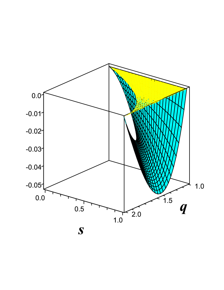
Fig. 1: (Color online) The function values of $m_{q,s}\left(1/\sqrt{2}\right)$ (patched blue curved surface) are indicated for real parameters $s$ and $q$. Yellow area on the top of the box indicates the range of $q$ and $s$ such that $1\leq q\leq 2$ and $-q^{2}+4q-3\leq s\leq 1$.

Now, we are ready to have the following theorem about the polygamy of multi-qubit entanglement using unified-$(q,s)$ entropy.

Theorem 1.

For $1\leq q\leq 2$, $-q^{2}+4q-3\leq s\leq 1$ and any multi-qubit state $\rho_{A_{1}\cdots A_{n}}$ , we have

$$E^{a}_{q,s}\left(\rho_{A_{1}(A_{2}\cdots A_{n})}\right)\leq E^{a}_{q,s}(\rho_{A_{1}A_{2}})+\cdots+E^{a}_{q,s}(\rho_{A_{1}A_{n}})$$ (47)

where $E_{q,s}\left(\rho_{A_{1}(A_{2}\cdots A_{n})}\right)$ is the unified-$(q,s)$ entanglement of $\rho_{A_{1}A_{2}\cdots A_{n}}$ with respect to the bipartition between $A_{1}$ and $A_{2}\cdots A_{n}$, and $E^{a}_{q,s}(\rho_{A_{1}A_{i}})$ is the UEoA of the reduced density matrix $\rho_{A_{1}A_{i}}$ for $i=2,\cdots,n$.

Proof.

We first prove the theorem for a $n$-qubit pure states, and generalize the proof into mixed states. For a $n$-qubit pure state ${\left|\psi\right\rangle}_{A_{1}(A_{2}\cdots A_{n})}$, let us first assume that $\mathcal{C}_{A_{1}(A_{2}\cdots A_{n})}^{2}\leq(\mathcal{C}^{a}_{A_{1}A_{2}})^{2}+(\mathcal{C}^{a}_{A_{1}A_{3}})^{2}+\cdots+(\mathcal{C}^{a}_{A_{1}A_{n}})^{2}\leq 1$ in Eq. (31). Then we have

$$E_{q,s}\left({\left|\psi\right\rangle}_{A_{1}(A_{2}\cdots A_{n})}\right) =f_{q,s}({\mathcal{C}}_{A_{1}(A_{2}\cdots A_{n})})$$

$$\leq f_{q,s}\left(\sqrt{(\mathcal{C}^{a}_{A_{1}A_{2}})^{2}+\cdots+(\mathcal{C}^{a}_{A_{1}A_{n}})^{2}}\right)$$

$$\leq f_{q,s}\left(\mathcal{C}^{a}_{A_{1}A_{2}}\right)$$

$$~{}+f_{q,s}\left(\sqrt{(\mathcal{C}^{a}_{A_{1}A_{3}})^{2}+\cdots+(\mathcal{C}^{a}_{A_{1}A_{n}})^{2}}\right)$$

$$~{}~{}~{}~{}~{}~{}~{}\vdots$$

$$\leq f_{q,s}\left(\mathcal{C}^{a}_{A_{1}A_{2}}\right)++\cdots+f_{q,s}\left(\mathcal{C}^{a}_{A_{1}A_{n}}\right)$$

$$\leq E_{q,s}^{a}\left(\rho_{A_{1}A_{2}}\right)+\cdots+E_{q,s}^{a}\left(\rho_{A_{1}A_{n}}\right),$$ (48)

where the first inequality is due to the monotonicity of the function $f_{q,s}(x)$, the second and third inequalities are obtained by iterative use of Lemma 2, and the last inequality is by Lemma 1.

Now, let us assume that $\mathcal{C}_{A_{1}(A_{2}\cdots A_{n})}^{2}\leq 1<(\mathcal{C}^{a}_{A_{1}A_{2}})^{2}+\cdots+(\mathcal{C}^{a}_{A_{1}A_{n}})^{2}$. Because $f_{q,s}(x)$ is an increasing function KSU , we have

$$E_{q,s}\left({\left|\psi\right\rangle}_{A_{1}(A_{2}\cdots A_{n})}\right)= f_{q,s}\left(\mathcal{C}_{A_{1}(A_{2}\cdots A_{n})}^{2}\right)$$

$$\leq f_{q,s}\left(1\right)$$ (49)

for any multi-qubit pure state ${\left|\psi\right\rangle}_{A_{1}(A_{2}\cdots A_{n})}$. Thus it is enough to show that $E_{q,s}^{a}(\rho_{A_{1}A_{2}})+\cdots+E_{q,s}^{a}(\rho_{A_{1}A_{n}})\geq f_{q,s}\left(1\right)$.

Our assumption $1<(\mathcal{C}^{a}_{A_{1}A_{2}})^{2}+\cdots+(\mathcal{C}^{a}_{A_{1}A_{n}})^{2}$ implies that there exists $k\in\{2,\ldots,n-1\}$ such that

$$(\mathcal{C}^{a}_{A_{1}A_{2}})^{2}+\cdots+(\mathcal{C}^{a}_{A_{1}A_{k}})^{2}\leq 1,$$

$$(\mathcal{C}^{a}_{A_{1}A_{2}})^{2}+\cdots+(\mathcal{C}^{a}_{A_{1}A_{k+1}})^{2}>1.$$ (50)

By letting

$$T:=(\mathcal{C}^{a}_{A_{1}A_{2}})^{2}+\cdots+(\mathcal{C}^{a}_{A_{1}A_{k+1}})^{2}-1>0,$$ (51)

we have

$$f_{q,s}\left(1\right)= f_{q,s}\left(1\right)$$

$$= f_{q,s}\left(\sqrt{(\mathcal{C}^{a}_{A_{1}A_{2}})^{2}+\cdots+(\mathcal{C}^{a}_{A_{1}A_{k+1}})^{2}-T}\right)$$

$$\leq f_{q,s}\left(\sqrt{(\mathcal{C}^{a}_{A_{1}A_{2}})^{2}+\cdots+(\mathcal{C}^{a}_{A_{1}A_{k}})^{2}}\right)$$

$$~{}~{}~{}~{}~{}~{}+f_{q,s}\left(\sqrt{(\mathcal{C}^{a}_{A_{1}A_{k+1}})^{2}-T}\right)$$

$$\leq f_{q,s}\left(\mathcal{C}^{a}_{A_{1}A_{2}}\right)+\cdots+f_{q,s}\left(\mathcal{C}^{a}_{A_{1}A_{k}}\right)+f_{q,s}(\mathcal{C}^{a}_{A_{1}A_{k+1}})$$

$$\leq E_{q,s}^{a}(\rho_{A_{1}A_{2}})+\cdots+E_{q,s}^{a}(\rho_{A_{1}A_{n}}),$$ (52)

where the first inequality is by using Lemma 2 with respect to $(\mathcal{C}^{a}_{A_{1}A_{2}})^{2}+\cdots+(\mathcal{C}^{a}_{A_{1}A_{k}})^{2}$ and $(\mathcal{C}^{a}_{A_{1}A_{k+1}})^{2}-T$, the second inequality is by iterative use of Lemma 2 on $(\mathcal{C}^{a}_{A_{1}A_{2}})^{2}+\cdots+(\mathcal{C}^{a}_{A_{1}A_{k}})^{2}$, and the last inequality is by Lemma 1.

Now let us consider multi-qubit mixed states. For a $n$-qubit mixed state $\rho_{A_{1}A_{2}\cdots A_{n}}$, let $\rho_{A_{1}(A_{2}\cdots A_{n})}=\sum_{j}p_{j}{\left|\psi_{j}\right\rangle}_{A_{1}(A_{2}\cdots A_{n})}{\left\langle\psi_{j}\right|}$ be an optimal decomposition for UEoA such that

$$E_{q,s}^{a}\left(\rho_{A_{1}(A_{2}\cdots A_{n})}\right)=\sum_{j}p_{j}E_{q,s}\left({\left|\psi_{j}\right\rangle}_{A_{1}(A_{2}\cdots A_{n})}\right).$$ (53)

Because each ${\left|\psi_{j}\right\rangle}_{A_{1}(A_{2}\cdots A_{n})}$ in the decomposition is an $n$-qubit pure state, we have

$$E_{q,s}\left({\left|\psi_{j}\right\rangle}_{A_{1}(A_{2}\cdots A_{n})}\right)\leq E_{q,s}^{a}\left(\rho^{j}_{A_{1}A_{2}}\right)+$$

$$\cdots+ E_{q,s}^{a}\left(\rho^{j}_{A_{1}A_{n}}\right)$$ (54)

where $\rho^{j}_{A_{1}A_{i}}$ is the reduced density matrix of ${\left|\psi_{j}\right\rangle}_{A_{1}\cdots A_{n}}$ onto two-qubit subsystem $A_{1}A_{i}$ for each $i=2,\cdots,n$. From Eq. (53) together with Inequality (54), we have

$$E_{q,s}^{a}\left(\rho_{A_{1}(A_{2}\cdots A_{n})}\right)= \sum_{j}p_{j}E_{q,s}\left({\left|\psi_{j}\right\rangle}_{A_{1}(A_{2}\cdots A_{n})}\right)$$

$$\leq \sum_{j}p_{j}E_{q,s}^{a}\left(\rho^{j}_{A_{1}A_{2}}\right)+\cdots$$

$$~{}~{}~{}~{}~{}~{}~{}~{}~{}~{}+\sum_{j}p_{j}E_{q,s}^{a}\left(\rho^{j}_{A_{1}A_{n}}\right)$$

$$\leq E_{q,s}^{a}\left(\rho_{A_{1}A_{2}}\right)+\cdots+E_{q,s}^{a}\left(\rho_{A_{1}A_{n}}\right),$$ (55)

where the last inequality is by definition of UEoA for each $\rho_{A_{1}A_{i}}$. ∎

We note that Inequality (47) is reduced to Tsallis-$q$ monogamy inequality KT

$${\mathcal{T}}^{a}_{q}\left(\rho_{A_{1}(A_{2}\cdots A_{n})}\right)\leq{\mathcal{T}}^{a}_{q}(\rho_{A_{1}A_{2}})+\cdots+{\mathcal{T}}^{a}_{q}(\rho_{A_{1}A_{n}})$$ (56)

as $s$ tends to 1, and it also reduces to the multi-qubit polygamy inequality in terms of EoA BGK as $q$ tends to 1. For $q=2$ and $s=1$, unified-$(q,s)$ entanglement coincides with the squared concurrence for two-qubit pure states; for a bipartite pure state ${\left|\psi\right\rangle}_{AB}$ with Schmidt-rank 2,

$$E_{2,1}\left({\left|\psi\right\rangle}_{AB}\right)={\mathcal{C}}^{2}\left({\left|\psi\right\rangle}_{AB}\right).$$ (57)

For this relation, it is also straightforward to verify that Inequality (47) reduces to Inequality (31) as $q\rightarrow 2$ and $s\rightarrow 1$. Thus, Theorem 1 provides an interpolation among EoA, TEoA and CoA polygamy inequalities of multi-qubit entanglement, which is illustrated in Figure 2.

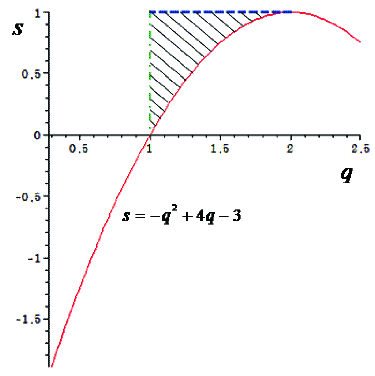
Fig. 2: (Color online) The domain of real parameters $q$ and $s$ where multi-qubit polygamy inequality holds in terms of UEoA. The dashed line indicates the domain for which the multi-qubit polygamy inequality holds for Tsallis-$q$ entropy (TEoA), and the dashed-dot line is the domain for von Neumann entropy (EoA). The shaded range is for unified-$(q,s)$ entropy (UEoA).

We further note that the continuity of unified-$(q,s)$ entropy also guarantees multi-qubit polygamy inequality in terms of UEoA when $q$ and $s$ are slightly outside of the proposed domain in Figure 2.

In three-qubit systems, Inequality (47) in Theorem 1 can be improved into a tighter form. A direct observation from ckw shows

$$\mathcal{C}_{A(BC)}^{2}=\mathcal{C}_{AB}^{2}+({\mathcal{C}^{a}_{AC}})^{2},$$ (58)

for a 3-qubit pure state ${\left|\psi\right\rangle}_{ABC}$ where $\mathcal{C}_{AB}$ and $\mathcal{C}^{a}_{AC}$ are the concurrence and CoA of $\rho_{AB}$ and $\rho_{AC}$ respectively.

From Eq. (58) together with Lemma 2, we have the following tighter polygamy inequality of three-qubit entanglement.

Theorem 2.

For $1\leq q\leq 2$, $-q^{2}+4q-3\leq s\leq 1$ and any three-qubit pure state ${\left|\psi\right\rangle}_{ABC}$, we have

$$E_{q,s}\left({\left|\psi\right\rangle}_{A(BC)}\right)\leq E_{q,s}(\rho_{AB})+E^{a}_{q,s}(\rho_{AC})$$ (59)

where $E_{q,s}\left({\left|\psi\right\rangle}_{A(BC)}\right)$ is the unified-$(q,s)$ entanglement of ${\left|\psi\right\rangle}_{ABC}$ with respect to the bipartition between $A$ and $BC$, $E_{q,s}(\rho_{AB})$ is the unified-$(q,s)$ entanglement of $\rho_{AB}$ and $E^{a}_{q,s}(\rho_{AC})$ is the UEoA of $\rho_{AC}$.

Proof.

Because ${\left|\psi\right\rangle}_{ABC}$ is a bipartite pure state between $A$ and $BC$ with Schmidt-rank less than or equal to two, we have

$$E_{q,s}\left(\psi_{A(BC)}\right)=f_{q,s}\left(\mathcal{C}_{A(BC)}\right).$$ (60)

Thus,

$$f_{q,s}\left(\mathcal{C}_{A(BC)}\right) =f_{q,s}\left(\sqrt{\mathcal{C}^{2}_{AB}+{\mathcal{C}^{a}_{AC}}^{2}}\right)$$

$$\leq f_{q,s}(\mathcal{C}_{AB})+f_{q,s}(\mathcal{C}^{a}_{AC})$$

$$\leq E_{q,s}(\rho_{AB})+E^{a}_{q,s}(\rho_{AC}),$$ (61)

where the first inequality is by Lemma 2, and the second inequality is by Lemma 1. ∎

IV Conclusion

Using unified-$(q,s)$ entropy, we have provided a two-parameter generalization of EoA, namely UEoA with an analytical lowerbound in two-qubit systems for $q\geq 1$, $0\leq s\leq 1$ and $qs\leq 3$. Based on this unified formalism of EoA, we have established a broad class of multi-qubit polygamy inequalities in terms of unified-$(q,s)$ entanglement for $1\leq q\leq 2$, $-q^{2}+4q-3\leq s\leq 1$. We have also shown a tighter polygamy inequality for the case of three-qubit pure states.

The class of polygamy inequalities we provided here encapsulates every known case of multi-qubit polygamy inequality in terms of EoA, CoA or TEoA as special cases, as well as their explicit relation with respect to a differential function $f_{q,s}(x)$. Thus our result provides a useful methodology to understand the restricted distribution of entanglement in multi-party quantum systems.

References

- (1) V. Coffman, J. Kundu and W. K. Wootters, Phys. Rev. A 61, 052306 (2000).
- (2) T. Osborne and F. Verstraete, Phys. Rev. Lett. 96, 220503 (2006).
- (3) M. Koashi and A. Winter, Phys. Rev. A 69, 022309 (2004).
- (4) B. M. Terhal, IBM J. Research and Development 48, 71 (2004).
- (5) A. J. Coleman and V. I. Yukalov, Lecture Notes in Chemistry Vol. 72 (Springer-Verlag, Berlin, 2000).
- (6) W. K. Wootters, Phys. Rev. Lett. 80, 2245 (1998).
- (7) J. S. Kim and B. C. Sanders, J. Phys. A: Math. and Theor. 43, 445305 (2010).
- (8) J. S. Kim, Phys. Rev. A. 81, 062328 (2010).
- (9) J. S. Kim and B. C. Sanders, J. Phys. A: Math. and Theor. 44, 295303 (2011).
- (10) J. S. Kim, A. Das and B. C. Sanders, Phys. Rev. A 79, 012329 (2009).
- (11) G. Gour, S. Bandyopadhay and B. C. Sanders, J. Math. Phys. 48, 012108 (2007).
- (12) T. Laustsen, F. Verstraete and S. J. van Enk, Quantum Inf. Comput. 3, 64 (2003).
- (13) F. Buscemi, G. Gour and J. S. Kim, Phys. Rev. A 80, 012324 (2009).
- (14) X. Hu and Z Ye, J. Math. Phys. 47, 023502 (2006).
- (15) A. E. Rastegin, J. Stat. Phys. 143, p. 1120–1135 (2011).
- (16) R. Horodecki, P. Horodecki and M. Horodecki, Phys. Lett. A 210, 377 (1996).
- (17) A. Rényi, Proceedings of the Fourth Berkeley Symposium on Mathematics, Statistics and Probability (University of California Press, Berkeley, 1961) 1, p. 547–561 .
- (18) C. Tsallis, J. Stat. Phys. 52, 479 (1988).
- (19) O. Cohen, Phys. Rev. Lett. 80, 2493 (1998).