A needlet ILC analysis of WMAP $9$-year polarisation data: CMB polarisation power spectra

Abstract

We estimate Cosmic Microwave Background (CMB) polarisation power spectra, and temperature-polarisation cross-spectra, from the $9$-year data of the Wilkinson Microwave Anisotropy Probe (WMAP). Foreground cleaning is implemented using minimum variance linear combinations of the coefficients of needlet decompositions of sky maps for all WMAP channels, to produce maps for CMB temperature anisotropies ($T$-mode) and polarisation ($E$-mode and $B$-mode), for $9$ different years of observation. The final power spectra are computed from averages of all possible cross-year power spectra obtained using foreground-cleaned maps for the different years. Our analysis technique yields a measurement of the $EE$ spectrum that is in excellent agreement with theoretical expectations from the current cosmological model. By comparison, the publicly available WMAP $EE$ power spectrum is higher on average (and significantly higher than the predicted $EE$ spectrum from the current best fit) at scales larger than about a degree, an excess that is not confirmed by our analysis. Our $TE$ and $TB$ measurements are in good agreement overall with the WMAP ones and are compatible with the theoretical expectations, although a few data points are off by a few standard deviations, and yield a reduced $\chi^{2}$ somewhat above expectation. As predicted for a standard cosmological model with low tensor to scalar ratio, the $EB$ and $BB$ power spectra obtained in our analysis are compatible with zero.

1 Introduction

The Cosmic Microwave Background (CMB), relic radiation emitted when our Universe was about 380,000 years old, provides direct information about the origin and history of cosmic structure. Hence, the current understanding of cosmological evolution is heavily based on observations of the CMB. Over the last two decades, many experiments have accumulated observations of its temperature anisotropies, imprints of the original density perturbations that later on gave rise to the large scale structures observable today. Two very successful space missions, the Cosmic Background Explorer (COBE, Bennett et al., 1996), and the Wilkinson Microwave Anisotropy Probe (WMAP, Bennett et al., 2003), complemented by several ground-based and balloon-borne experiments, such as CAT (Baker et al., 1999), Boomerang (de Bernardis et al., 2000), Maxima (Hanany et al., 2000), Archeops (Benoît et al., 2003a, b), CBI (Pearson et al., 2003), VSA (Dickinson et al., 2004; Rebolo et al., 2004), ACBAR (Reichardt et al., 2009), ACT (Das et al., 2011a, b), and SPT (Keisler et al., 2011), to mention just a few, have measured the CMB temperature anisotropies at various angular scales and at various wavelengths. Recently, the Planck collaboration has released a precise measurement of the CMB temperature power spectrum (Planck collaboration XV, 2013) which led to an update of the best fit cosmological parameters (Planck Collaboration XVI, 2013).

The CMB angular power spectra measured by these experiments strongly support a present cosmological model in which the Universe is spatially flat, with an energy density dominated by the presence of about 70% dark energy and about 30% matter, and in which structure forms from gravitational collapse of primordial adiabatic perturbations in the density of the cosmological fluid. At present, this model does not require the additional admixture of primordial tensor perturbations (gravitational waves), although cosmological scenarios generically predict their existence. The observed CMB anisotropies are connected to the state of the cosmological fluid at recombination in a way that depends on a small set of parameters specific of the cosmological model. CMB observations are of prime importance for constraining these parameters of the model, as well as for testing its internal consistency.

Temperature anisotropies alone, however, do not provide the complete picture of the Universe. Independent information is needed to lift degeneracies between cosmological parameter sets compatible with the CMB temperature power spectrum. Other cosmological probes such as the direct measurement of the present expansion rate (Freedman et al., 2001), the observation of the expansion history with supernova (Perlmutter et al., 1999; Astier et al., 2006; Guy et al., 2010), or baryonic oscillations traced by the distribution of galaxies (Eisenstein et al., 2005), provide complementary constraints (Seljak, Slosar, & McDonald, 2006).

On the side of the CMB itself, additional informations are obtained by measuring CMB polarisation. The CMB is indeed partially polarised due to Thomson scattering of quadrupolar distribution of photons on free electrons at the time of recombination (Rees, 1968), at a redshift $z_{\rm rec}$ of about $1100$. Large scale polarisation also arises from the scattering of CMB photons on free electrons after reionisation of the Universe at much lower redshift ($z_{\rm reion}<10$). CMB polarisation is an additional observable, which helps disentangling Sachs-Wolfe from Doppler contributions to the anisotropies, makes possible the estimation of individual contributions to the power spectra from scalar and tensor perturbations, and also helps constraining the epoch of reionisation. The amplitude of the polarisation, however, is significantly lower than that of temperature anisotropies, which makes its precise characterisation challenging.

CMB polarisation was first detected at sub-degree angular scales by the DASI ground-based interferometer (Leitch et al., 2005). It was subsequently measured by Boomerang (Montroy et al., 2006; Piacentini et al., 2006), Maxipol (Wu et al., 2007), CBI (Sievers et al., 2007), CAPMAP (Bischoff et al., 2008), QUaD (Pryke et al., 2009; Brown et al., 2009), BICEP (Chiang et al., 2010), QUIET (QUIET Collaboration et al., 2011), and the Wilkinson Microwave Anisotropy Probe (WMAP, Nolta et al., 2009; Larson et al., 2011).

The level of the CMB polarisation (at most a few per cent, depending on the angular scale), however, makes it easily contaminated by foreground emissions from both the Galaxy and extragalactic sources. Galactic emission, in particular, is polarised at the level of a few tens of per cent, i.e. ten times more than CMB anisotropies. The signal to foreground ratio is thus less favourable for polarisation than for intensity, in particular on large angular scales where Galactic synchrotron and dust emissions are strong. Contamination by foregrounds would result in CMB polarisation power spectra larger than predicted by the current cosmological model. For WMAP, the main contaminant is synchrotron emission, but even dust, which has been measured to be polarised at a level that can exceed 10% (Benoît et al., 2004), is a potential worry.

Hence, contamination from polarised foreground signals has to be removed as much as possible for the accurate measurement of the temperature and polarisation angular power spectrum of the CMB. The effectiveness of a foreground cleaning technique is typically significantly improved by the use of prior knowledge of the emission properties of the contaminant (such as the frequency dependence, typical angular power spectrum of its emission, or availability of external templates). However, since the properties of foreground contamination are poorly known for polarisation (and, in particular, no good template of polarised foregrounds is presently available), it is particularly crucial to develop and use data analysis tools that use only the minimum possible prior assumptions about foreground polarisation.

Among the possible methods for CMB cleaning, the so-called Internal Linear Combination (ILC) method, first proposed for foreground cleaning in the analysis of COBE-DMR data (Bennett et al., 1992), and discussed subsequently by many authors (see, e.g., Tegmark, 1998), is a simple and effective way to combine multifrequency observations to extract the CMB while rejecting contamination by superimposed foreground signals. This method is based on two reasonably safe assumptions. The first is that the amplitude of CMB emission is frequency independent in thermodynamic units, i.e. that the CMB emission law scales in frequency as the derivative of the blackbody spectrum of the cosmic background. The second is that CMB fluctuations are not correlated to foreground signals. Under these assumptions, the ILC estimates the CMB as a linear combination of sky maps such that the variance of the estimate is minimum, while preserving unit response to the CMB (see, however, the appendix of Delabrouille et al. (2009) for a discussion of second order corrections and biases, and Dick, Remazeilles, & Delabrouille (2010) for a discussion of the impact of calibration errors).

Component separation with an ILC method can be straightforwardly implemented either in real space or in harmonic space (Tegmark, de Oliveira-Costa, & Hamilton, 2003; Eriksen et al., 2004; Saha, Jain & Souradeep, 2006; Souradeep, Saha., Jain, 2006; Saha, Prunet, Jain & Souradeep, 2008; Saha, 2011; Souradeep, 2011). Here, as in our previous work (Delabrouille et al., 2009; Basak & Delabrouille, 2012), we instead implement the ILC on a frame of spherical wavelets, called needlets. This special type of wavelets on the sphere provides good localisation in both pixel space and harmonic space because they have compact support in the harmonic domain, while still being very well localised in the pixel domain (Narcowich, Petrushev & Ward, 2006; Marinucci et al., 2008; Guilloux, Faÿ, & Cardoso, 2009). Needlets have already been used in various analyses of WMAP data besides component separation and power spectrum estimation, for instance by Pietrobon et al. (2008) to detect features in the CMB, and by Rudjord et al. (2009) to put limits on the non-Gaussianity parameter $f_{\rm NL}$.

Recently, we have used a needlet ILC on WMAP $7$-year data to obtain an estimate of the CMB temperature angular power spectrum (Basak & Delabrouille, 2012). In the present paper, as a natural extension to this work, we address the problem of measuring the CMB polarisation power spectra, and temperature-polarisation cross-spectra from WMAP $9$-year observations as precisely as possible.

The paper is organised as follows: In section 2 we describe the methodology to estimate the CMB using an ILC on wavelet decompositions of multi-frequency sky maps. The implementation of this on WMAP $9$-year data, and the results for polarisation power spectra, are described in sections 3, 4 and 5. We conclude in section 6.

2 Needlet ILC estimate of CMB

A scalar field on the sphere such as CMB temperature anisotropies is conveniently expanded in usual spherical harmonics:

$$T(\hat{n})=\sum_{l=0}^{\infty}\sum_{m=-l}^{l}T_{lm}Y_{lm}(\hat{n})$$ (1)

The CMB polarisation field is usually specified using the Stokes parameters, $Q$ and $U$, with respect to a particular choice of a coordinate system on the sky in relation to which the linear polarisation is defined. One can conveniently combine the Stokes parameters into the single complex quantity, $P_{\pm}=Q\pm iU$. Due to its rotation properties, one may expand $P_{\pm}(\hat{n})$ in terms of spin-$2$ spherical harmonics, ${}_{\pm 2}Y_{lm}(\hat{n})$ (Goldberg et al., 1967), as:

$$P_{\pm}(\hat{n})=\sum_{l=0}^{\infty}\sum_{m=-l}^{l}P_{\pm 2,lm}\,{}_{\pm 2}Y_{lm}(\hat{n}).$$ (2)

The description of CMB polarisation, however, traditionally makes use of two scalar fields that are independent of how the coordinate system is oriented, and are related to the Stokes parameters by a non-local transformation (Zaldarriaga & Seljak, 1997; Kamionkowski, Kosowsky, & Stebbins, 1997). One of the fields, traditionally denoted as $E$, has even parity, whereas the other one, $B$, has odd parity (and hence is pseudo-scalar, rather than scalar). In harmonic space, the $E$ and $B$ modes of CMB polarisation are related to the complex polarisation fields $P_{\pm}$ as,

$$P_{+2,lm}=-(E_{lm}+iB_{lm})$$ (3)

and

$$P_{-2,lm}=-(E_{lm}-iB_{lm}).$$ (4)

Hence, one can fully characterise CMB anisotropies using three Gaussianly distributed random scalar fields ($T$, $E$ and $B$), without loss of information. In the following, maps of $Q$ and $U$ are converted into maps of $E$ and $B$ by expansion onto spin-$2$ spherical harmonics, followed by an inverse spherical harmonic transform for $E_{lm}$ and $B_{lm}$ independently.

2.1 The CMB data model

Denote $X^{\text{OBS},c}(\hat{n})$, $(X={T,E,B})$ full-sky, multi-frequency temperature anisotropy and polarisation maps of the sky in $n_{c}$ different frequency bands (channels), such as those provided by WMAP. The observed signal $X^{\text{OBS},c}(\hat{n})$ in channel $c$ can be modelled as,

$$X^{\text{OBS},c}(\hat{n})=\int_{\hat{n}^{\prime}}d\Omega_{\hat{n}^{\prime}}\,\,b^{c}(\hat{n}.\hat{n}^{\prime})\,\,X^{\text{SIG},c}(\hat{n}^{\prime})+X^{\text{N},c}(\hat{n})$$ (5)

where $X^{\text{SIG},c}(\hat{n})$ is the signal (sky) component, itself decomposed in the sum of CMB and foreground components,

$$X^{\text{SIG},c}(\hat{n})=a^{c}\,X^{\text{CMB}}(\hat{n})+X^{\text{FG},c}(\hat{n}),$$ (6)

$a^{c}$ being the CMB calibration coefficient for the channel $c$. Up to calibration uncertainties, $a^{c}=1$ for all WMAP channels. If, in addition to WMAP data, we use external data sets which serve as foreground templates to help foreground subtraction, as done in the present work, the coefficients $a^{c}$ vanish for such data sets (i.e. the ancillary maps contain no CMB anisotropies).

The beam function $b^{c}(\hat{n}.\hat{n}^{\prime})$, represents the smoothing of the signal due to the finite resolution of the observations. Assuming for simplicity that the beams are circularly symmetric (a good approximation for WMAP data), $b^{c}(\hat{n}.\hat{n}^{\prime})$ depends only on the angle $\theta=\cos^{-1}(\hat{n}.\hat{n}^{\prime})$ between the directions $\hat{n}$ and $\hat{n}^{\prime}$, and can be expanded in terms of Legendre polynomials,

$$b^{c}(\hat{n}.\hat{n}^{\prime})=\sum_{l=0}^{\infty}\frac{2l+1}{4\pi}b_{l}^{c}P_{l}(\hat{n}.\hat{n}^{\prime}).$$ (7)

The last term, $X^{\text{N},c}(\hat{n})$, in equation (5) represents the detector noise in channel $c$, and is not affected by the beam function. For a spherically symmetric beam, equation 5 can be recast straightforwardly in the spherical harmonic representation, as:

$$X_{lm}^{\text{OBS},c}=a^{c}\,b_{l}^{c}\,X_{lm}^{\text{CMB}}+b_{l}^{c}\,X_{lm}^{\text{FG},c}+X_{lm}^{\text{N},c}$$ (8)

where $X_{lm}$ stands for the three modes $T_{lm}$, $E_{lm}$ and $B_{lm}$ of temperature and polarisation in harmonic space.

2.2 Implementation of the needlet transform

Considering that each channel observes the sky at a different resolution, the maps are first convolved/deconvolved, in harmonic space, to the same resolution:

$$X_{lm}^{c}=\frac{b_{l}}{b_{l}^{c}}\,\,X_{lm}^{\text{OBS},c}.$$ (9)

Each of these maps $X_{lm}^{c}$ is then decomposed into a set of filtered maps $X_{lm}^{c,j}$ represented by the spherical harmonic coefficients,

$$X_{lm}^{c,j}=h_{l}^{j}X_{lm}^{c},$$ (10)

where the filters $h_{l}^{j}$, serving for localisation in the harmonic space, are chosen in such a way that

$$\sum_{j}\left(h_{l}^{j}\right)^{2}=1.$$ (11)

The reconstruction of the original maps $X_{lm}^{c}$ from the collection of the filtered maps $X_{lm}^{c,j}$, representing each a different scale, is performed using the same set of filters. In terms of $h_{l}^{j}$, the spherical needlets are defined as,

$$\Psi_{jk}(\hat{n})=\sqrt{\lambda_{jk}}\sum_{l=0}^{l_{\max}}\sum_{m=-l}^{l}h_{l}^{j}\,Y_{lm}^{*}(\hat{n})\,Y_{lm}(\hat{\xi}_{jk}),$$ (12)

where $\{\xi_{jk}\}$ denote a set of cubature points on the sphere for scale $j$. In practice, we identify these points with the pixel centres in the HEALPix pixelisation scheme (Górski et al., 2005). Each index $k$ corresponds to a particular HEALPix pixel, at a resolution parameter nside$(j)$ specific to that scale $j$. The cubature weights $\lambda_{jk}$ are inversely proportional to the number $N_{j}$ of pixels used for the needlet decomposition, i.e. $\lambda_{jk}=\frac{4\pi}{N_{j}}$. The needlet coefficients for CMB fields $X(\hat{n})$ are denoted as,

$$\beta^{X}_{jk} = \int_{S^{2}}X(\hat{n})\,\Psi_{jk}(\hat{n})\,d\Omega_{\hat{n}}$$ (13)

$$= \sqrt{\lambda_{jk}}\sum_{l=0}^{l_{\max}}\sum_{m=-l}^{l}h_{l}^{j}\,b_{l}\,X_{lm}\,\,Y_{lm}(\xi_{jk}).$$

The linearity of the needlet decomposition implies that the needlet coefficients $\beta_{jk}^{c}$ corresponding to the filtered map obtained from the harmonic coefficients $X_{lm}^{c,j}$ are a linear combination of the needlet coefficients of individual components and noise at HEALPix grid points $\xi_{jk}$:

$$\beta_{jk}^{X,c}=a^{c}\,\beta_{jk}^{\text{CMB}}+\beta_{jk}^{\text{FG},c}+\beta_{jk}^{\text{N},c}$$ (14)

where,

$$\beta_{jk}^{\text{CMB}} = \sqrt{\lambda_{jk}}\sum_{l=0}^{l_{\max}}\sum_{m=-l}^{l}h_{l}^{j}\,b_{l}\,X_{lm}^{\text{CMB}}\,\,Y_{lm}(\xi_{jk})$$

$$\beta_{jk}^{\text{FG},c} = \sqrt{\lambda_{jk}}\sum_{l=0}^{l_{\max}}\sum_{m=-l}^{l}h_{l}^{j}\,b_{l}\,X_{lm}^{\text{FG},c}\,\,Y_{lm}(\xi_{jk})$$

$$\beta_{jk}^{\text{N},c} = \sqrt{\lambda_{jk}}\sum_{l=0}^{l_{\max}}\sum_{m=-l}^{l}h_{l}^{j}\,\frac{b_{l}}{b_{l}^{c}}\,X_{lm}^{\text{N},c}\,\,Y_{lm}(\xi_{jk})$$ (15)

2.3 Implementation of the needlet ILC

The ILC estimate of needlet coefficients of the cleaned map is obtained as a linearly weighted sum of the needlet coefficients $\beta_{jk}^{c}$,

$$\beta_{jk}^{\text{NILC}}=\sum_{c=1}^{n_{c}}\omega_{jk}^{c}\,\beta_{jk}^{X,c}$$ (16)

where $\omega_{jk}^{c}$ is the needlet weight for scale $j$ and frequency channel $c$, at the pixel $k$ of the HEALPix representation of the needlet coefficients for that scale. Under the assumption of decorrelation between CMB and foregrounds, and between CMB and noise, the empirical variance of the error is minimum when the empirical variance of the ILC map itself is minimum. The condition for preserving the CMB signal during the cleaning is encoded as the constraint:

$$\sum_{c=1}^{n_{c}}a^{c}\omega_{jk}^{c}=1.$$ (17)

The resulting needlet ILC weights $\widehat{\omega}_{jk}^{c}$ that minimise the variance of the reconstructed CMB, subject to the constraint that the CMB is preserved, are expressed as:

$$\widehat{\omega}_{jk}^{c}=\frac{\sum_{c^{\prime}}\left[\widehat{R}_{jk}^{-1}\right]^{cc^{\prime}}a^{c^{\prime}}}{\sum_{c}\sum_{c^{\prime}}a^{c}\left[\widehat{R}_{jk}^{-1}\right]^{cc^{\prime}}a^{c^{\prime}}},$$ (18)

where indices $c$ and $c^{\prime}$ of elements of the matrix $\left[\widehat{R}_{jk}^{-1}\right]$ and of the vectors $\widehat{\omega}_{jk}$ and $a$ are written down explicitly for clarity. More compactly, we have:

$$\widehat{\omega}_{jk}=\frac{\left[\widehat{R}_{jk}^{-1}\right]a}{a^{T}\left[\widehat{R}_{jk}^{-1}\right]a},$$ (19)

where $\widehat{\omega}_{jk}$ is the vector of ILC weights to be applied to the needled coefficients of all input observations at scale $j$ and in pixel $k$, $a$ is the CMB ‘mixing vector’ (a vector of $n_{c}$ entries all equal to unity for inputs in thermodynamic temperature), and $\left[\widehat{R}_{jk}^{-1}\right]$ an estimate of the inverse covariance of the needlet coefficients of the $n_{c}$ observations at pixel $k$ of scale $j$.

The NILC estimate of the cleaned CMB needlet coefficients is:

$$\beta_{jk}^{\text{NILC}}=\beta_{jk}^{\text{CMB}}+\sum_{c}\widehat{\omega}_{jk}^{c}\left(\beta_{jk}^{\text{FG},c}+\beta_{jk}^{\text{N},c}\right).$$ (20)

The elements of the covariance matrix for scale $j$ at pixel $k$, $R_{jk}^{cc^{\prime}}=\left<\beta_{jk}^{c}\beta_{jk}^{c^{\prime}}\right>$, are obtained each as an average of the product of the relevant computed needlet coefficients over some space domain ${\cal D}_{k}$ centred at $k$. In practice, they are computed as

$$\widehat{R}_{X,jk}^{cc^{\prime}}=\frac{1}{n_{k}}\sum_{k^{\prime}}w_{j}(k,k^{\prime})\,\beta_{jk}^{X,c}\beta_{jk}^{X,c^{\prime}},$$ (21)

where the weights $w_{j}(k,k^{\prime})$ define the domain ${\cal D}_{k}$. A sensible choice is for instance $w_{j}(k,k^{\prime})=1$ for $k^{\prime}$ closer to $k$ than some limit angle, and $w_{j}(k,k^{\prime})=0$ elsewhere, or alternatively, $w_{j}(k,k^{\prime})$ shaped as a Gaussian beam of some given size that depends on the scale $j$ (which is what we do here).

Finally, the NILC estimate of the cleaned CMB map can be reconstructed from cleaned CMB needlet coefficients using the same set of filters that was used to decompose the original maps into their needlet coefficients. The NILC CMB map is then

$$X^{\text{NILC}}(\hat{n}) = \sum_{lm}X_{lm}^{\text{NILC}}\,Y_{lm}(\hat{n})$$ (22)

with

$$X_{lm}^{\text{NILC}}=b_{l}\,X_{lm}^{\text{CMB}}+X_{lm}^{\text{RFG}}+X_{lm}^{\text{RN}},$$ (23)

where the harmonic coefficients residual foreground ($X_{lm}^{\text{RFG}}$) and residual noise ($X_{lm}^{\text{RN}}$) are given by:

$$X_{lm}^{\text{RFG}}=\sum_{j}\sum_{k}\sqrt{\lambda_{jk}}\,\beta_{jk}^{\text{RFG}}\,h_{l}^{j}\,Y_{lm}(\xi_{jk})$$ (24)

and

$$X_{lm}^{\text{RN}}=\sum_{j}\sum_{k}\sqrt{\lambda_{jk}}\,\beta_{jk}^{\text{RN}}\,h_{l}^{j}\,Y_{lm}(\xi_{jk}).$$ (25)

Equations 22 and 23 imply that the NILC estimate of CMB contains some residual foreground and noise contamination.

3 WMAP $9$-year needlet ILC map

The WMAP satellite has observed the sky in five frequency bands denoted K, Ka, Q, V and W, centred at $23$, $33$, $41$, $61$ and $94$ GHz respectively. After $9$ years of observation, the released data includes temperature anisotropy and polarisation maps obtained with ten difference assemblies, for $9$ individual years. One map is available, per year, for each of the K and Ka bands, two for the Q band, two for the V band and four for the W band. These sky maps are sampled using the HEALPix pixelisation scheme at a resolution level (nside$=512$), corresponding to approximately $3$ million sky pixels.

We work on band-averaged maps of $T$, $E$ and $B$ for the five frequency bands, complemented, for temperature only, by three foreground templates (dust at $100$ microns, as obtained by Schlegel, Finkbeiner, & Davis (1998), the $408$ MHz synchrotron map of Haslam et al. (1981), and the composite all-sky H-alpha map of Finkbeiner (2003)). All sky maps are convolved/deconvolved in harmonic space, to a common beam resolution (full width at half maximum (FWHM)$=13.2$).

Each of these maps is then decomposed into a set of needlet coefficients. For each scale $j$, needlet coefficients of a given map are stored in the format of a single HEALPix map at degraded resolution. The filters $h^{j}_{l}$ used to compute filtered maps are shaped as follows:

$$h^{j}_{l}=\left\{\begin{array}[]{rl}\cos\left[\left(\frac{l^{j}_{peak}-l}{l^{j}_{peak}-l^{j}_{min}}\right)\frac{\pi}{2}\right]&\text{for }l^{j}_{min}\leq l<l^{j}_{peak},\\ \\ 1&\text{for }l=l_{peak},\\ \\ \cos\left[\left(\frac{l-l^{j}_{peak}}{l^{j}_{max}-l^{j}_{peak}}\right)\frac{\pi}{2}\right]&\text{for }l^{j}_{peak}<l\leq l^{j}_{max}\end{array}\right.$$

For each scale $j$, the filter has compact support between the multipoles $l^{j}_{min}$ and $l^{j}_{max}$ with a peak at $l^{j}_{peak}$ (see figure 1 and table 1). The needlet coefficients $\beta^{X}_{jk}$ are computed from these filtered maps on HEALPix grid points $\xi_{jk}$ with resolution parameter nside equal to the smallest power of $2$ larger than $l^{j}_{max}/2$.

Table 1: List of needlet bands used in the present analysis.

Band index	$l_{min}$	$l_{peak}$	$l_{max}$	nside
1	0	0	50	32
2	0	50	100	64
3	50	100	150	128
4	100	150	250	128
5	150	250	350	256
6	250	350	550	512
7	350	550	650	512
8	550	650	800	512
9	650	800	1000	512

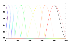
Figure 1: The broken lines show the needlet bands used in the present analysis. The solid black line shows the normalisation of the needlet bands, i.e. the total filter applied to the original map after needlet decomposition and synthesis of the output map from needlet coefficients.

The estimates of needlet coefficients covariance matrices, for each scale $j$, are computed by smoothing maps of products of needlet coefficient $\beta^{c}_{jk}\beta^{c^{\prime}}_{jk}$ with Gaussian beams. In this way, an estimate of needlet covariances at each point $k$ is obtained as a local, weighted average of nearby needlet coefficient products. The full width at half maximum (FWHM) of each of the Gaussian windows used for this purpose is chosen to ensure the computation of the statistics by averaging about $1200$ samples or more, resulting from a trade-off between the localisation of the estimates (which requires small windows), and the accuracy of the estimate (which require large windows). Choosing a smaller FWHM results in inaccuracy in the covariance estimates, and hence ILC bias. Choosing a larger FWHM results in less localisation, and hence loss of effectiveness of the needlet approach.

Using these covariance matrices, ILC weights are computed for each of $T$, $E$ and $B$, for each scale $j$ and for each pixel $k$ of the needlet representation at scale $j$. For each of $T$, $E$ and $B$, a full sky CMB map, at the resolution of the WMAP W channel, is synthesised from the NILC needlet coefficients.

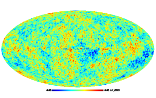
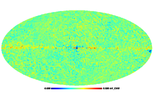
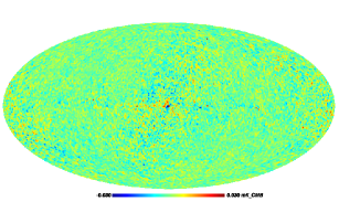
Figure 2: The NILC estimate of temperature anisotropies(top) and, Stokes parameters $Q$ (middle) and $U$ (bottom) of CMB obtained by implementing the NILC on the $9$-year band average maps, at nside$~{}=~{}512$ and degraded to $60$ arcmin resolution.

4 WMAP $9$-year needlet ILC spectrum

As already mentioned above, the foreground-cleaned maps of $T$, $E$ and $B$ obtained in this way are not fully exempt from contamination by residual foregrounds and noise. The recovered CMB map ($T$, $Q$ and $U$) at $60$ arcmin resolution is displayed in figure 2. Residual foreground contamination, albeit small, is visible along a narrow strip on the Galactic plane of these maps. Noise contamination is seen from the larger variance of the polarisation maps away from the ecliptic poles. Note, however, that these maps have been obtained with no masking whatsoever of the original data sets. We rely on the localisation provided by the needlets to avoid more contaminated sky areas to impact the reconstruction of the CMB over the rest of the sky. That choice, even if probably sub-optimal, is easy to implement, and turns out to be good enough for the analysis of WMAP observations.

4.1 Minimisation of the impact of noise

Noise biasing in our estimated power spectra is avoided by producing, for each of $T$, $E$ and $B$, an independent CMB map for each of the $9$ individual years of observation. All maps, however, are obtained using the same set of needlet weights, determined using the co-added $9$ year observations. To avoid the bias induced by residual instrumental noise in the maps, we compute the CMB power spectra exclusively from cross-products between maps from different years. Each data point in our spectra is thus obtained as an average of all possible cross-year spectra ($72$, although in the case of $EE$ and $BB$ half of those are strictly identical to the other half). We take into account the correlation between errors in the $72$ cross-spectra estimates for the final average spectrum (see appendix for details).

4.2 Minimisation of the impact of foregrounds

Unlike the residual noise, the residual foreground emission in each of $9$ cleaned maps is the same, as each map observes the same sky emission, and is produced using the same linear combination for all years.

We use the conservative temperature and polarisation analysis masks provided by the WMAP collaboration, applied directly on the CMB maps after the needlet ILC. We choose this option (rather than masking before the ILC) so that we produce full sky CMB maps that can also be used for other purposes than power spectrum estimation. In order to correct for the sky fraction we use here the MASTER method (Hivon et al., 2002) to compute the power spectrum.

4.3 The effectiveness of the NILC

The NILC approach automatically adjusts weights of the linear combination input sky maps as a function of sky area and of angular scale (i.e. in regions of pixel-scale space), to minimise the overall contamination by any signal that does not have the expected colour of the CMB. This includes astrophysical foregrounds, but also instrumental noise and even residual additive systematic effects.

For instance, in a pixel-scale region where instrumental noise dominates the error in the observations (i.e. with negligible foregrounds), the NILC is in effect equivalent to a noise-weighted average of all WMAP maps. All the ILC weights are positive, proportional to the inverse of the noise power of the various channels in that region.

On the other hand, in a pixel-scale region significantly contaminated by foregrounds, the NILC coefficients adjust themselves automatically to minimise the total variance of the error, i.e. use positive and negative coefficients to cancel-out the foregrounds (in a compromise between noise and foreground contamination).

Finally, the NILC is even effective at minimising the contamination by unknown additive residual systematics. Imagine that one particular channel suffers from such residuals in one particular pixel-scale region. The NILC will automatically minimise the weight of that particular channel in the linear combination for that region (and, possibly, the weight of another channel in another region, if that turns out to be necessary).

4.4 Impact of calibration errors

An important assumption of the ILC is that the frequency scaling of the CMB is known. However, calibration coefficients for each channel, which are a multiplicative factor for each frequency, introduce an uncertainty in the frequency scalings of the CMB component in the presence of calibration errors (Dick, Remazeilles, & Delabrouille, 2010). This effect is particularly strong in the high signal to noise ratio regime. Considering the relatively low signal to noise of WMAP polarised maps, this issue can safely be ignored here.

Beam uncertainties induce similar biases as calibration uncertainties, except that these biases are scale dependent. Here again, such biases are not the main source of error in our final polarisation spectra, as their impact is small in comparison to the uncertainties due to instrumental noise for polarisation measurements with WMAP.

These issues, connected to the exact response of the detectors, however, will require specific attention with upcoming more sensitive observations of the polarised CMB, if our method is to be used for the analysis of these future data sets.

4.5 Noise-weighting

Residual noise in our CMB maps is inhomogeneous, primarily because of non-uniform sky coverage, with higher number of observations in the directions of ecliptic poles and rings at $45^{\circ}$ ecliptic latitude.

At multipoles where noise is the main source of error, there is advantage to weighting the maps with the inverse noise variance for computing the power spectrum. This amounts to giving more weight in the final spectrum estimate to regions of the sky less contaminated by noise. At large angular scales, however, cosmic variance dominates, and it is preferable to use uniform weighting.

Considering this, we compute all power spectra using both schemes, for all multipole bins. In practice, the map of weights for the noise-weighted scheme is obtained using the map of number of hits of the W-channel (maps for all channels are similar).

For both cases (noise weighted and uniform weighting), we compute the error bar on our estimate of CMB power spectra as described in the appendix. We then pick, for the final power spectrum, that of the two with the lowest variance. In the case of $TE$ and $TB$, the uniform weighting is better in the first 24 multipole bins (below $l=317$). For $EE$, $BB$ and $EB$, the noise-weighted estimate is better in all multipole bins.

An alternative to this noise-weighting method would be to use the optimised needlet weighting approach investigated for intensity maps in a method paper by Faÿ et al. (2008), which pushes the optimisation yet one step further and is used in our previous analysis of WMAP intensity maps (Basak & Delabrouille, 2012). However, the extra complication involved is not necessary here, as it does not make much difference for a data set in which the noise is not too inhomogeneous (as is the case in the present data set).

4.6 Results

We now present the estimated polarisation power spectra and temperature-polarisation cross power spectra obtained on the basis of WMAP $9$-year observations. The error bars in our estimates (see appendix for details) include the total statistical error of the estimator (noise and cosmic variance terms). The measurement of the variance of CMB power spectra, requires an estimate of the power spectrum of the esidual noise present in NILC-CMB maps (see Appendix for details). This estimation could be made with a blind method such as SMICA (Delabrouille et al., 2003; Cardoso et al., 2008), which provides a maximum-likelihood multi-component fit to an empirical estimate of the multi-varied power spectrum of several independent observations of CMB contaminated by foegrounds and noise. Here, we perform a simpler estimation in three steps. First, we average all possible single-year measurements power spectra, corrected for the effect of the mask using the MASTER method. Then, we estimate the noise level from the difference of this measurement based on on-diagonal terms, and of the CMB power spectrum inferred from off-diagonal terms in the maps covariance. Finally, we obtain the variance of CMB power spectra from this together with best-fit theoretical power spectra, using equation 41. We correct our error estimates for partial sky coverage by dividing the variance of measured angular power spectra by the corresponding sky fraction (equation 42 and 43).

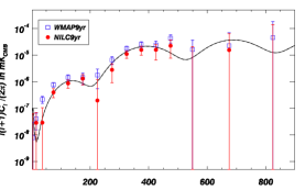
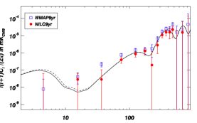
Figure 3: The red filled circles show the angular power spectrum of $E$-mode of CMB polarisation as estimated with our method using $9$ years of observations of WMAP. The dark blue open squares show the $9$-year angular power spectrum of $E$-mode of CMB polarisation published by the WMAP collaboration. The solid black line shows the theoretical angular power spectrum for WMAP best-fit $\Lambda$-CDM model (Hinshaw et al., 2013). The broken black line shows the theoretical angular power spectrum for Planck best-fit $\Lambda$-CDM model (Planck Collaboration XVI, 2013). The top panel uses a linear scale in the horizontal axis, and the bottom panel a logarithmic scale.

Table 2: Comparison of our estimate of binned angular power spectrum of $E$-mode of CMB polarisation with that provided by WMAP team. The quantities tabulated are $D_{l}=l(l+1)C_{l}^{EE}/2\pi$ and $\Delta D_{l}=l(l+1)\Delta C_{l}^{EE}/2\pi$.

$l_{\rm range}$	$D_{l}^{\rm nilc}$	$D_{l}^{\rm wmap}$	$\Delta D_{l}^{\rm nilc}$	$\Delta D_{l}^{\rm wmap}$
	$(mK^{2})$	$(mK^{2})$	$(mK^{2})$	$(mK^{2})$
2–7	-1.378e-08	7.917e-09	6.776e-08	2.191e-08
8–23	1.323e-08	4.035e-08	4.700e-08	2.496e-08
24–49	8.213e-09	2.159e-07	8.574e-08	6.396e-08
50–99	3.574e-07	7.733e-07	1.679e-07	1.452e-07
100–149	7.732e-07	1.453e-06	3.329e-07	3.457e-07
150–199	1.493e-06	1.441e-06	6.169e-07	6.721e-07
200–249	-3.088e-07	1.769e-06	1.142e-06	1.223e-06
250–299	2.289e-06	6.583e-06	2.111e-06	2.160e-06
300–349	9.964e-06	1.783e-05	3.928e-06	3.673e-06
350–399	1.145e-05	2.572e-05	6.534e-06	6.007e-06
400–449	1.326e-05	2.431e-05	1.050e-05	9.510e-06
450–499	2.051e-05	4.327e-05	1.667e-05	1.478e-05
500–599	-4.335e-05	1.609e-05	2.352e-05	2.055e-05
600–749	1.814e-05	2.289e-05	5.443e-05	4.718e-05
750–898	-2.773e-04	4.548e-05	1.594e-04	1.367e-04

4.6.1 $EE$ angular power spectrum

Figure 3 shows the estimated auto-angular power spectrum for the $E$-mode of CMB polarisation. Our estimated $E$-mode CMB power is lower than that obtained by the WMAP collaboration, in all of the multipole bins, and in better agreement with the theoretical expectations (assuming the cosmological model is correct) (see table 2). The systematic difference between our measurement and that of the WMAP team is presently not understood. We suspect that their estimate is contaminated by residual foreground emission or systematics.

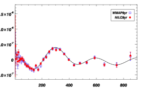
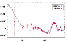
Figure 4: The red filled circles show the cross-angular power spectrum of CMB temperature anisotropies ($T$-mode) and $E$-mode of CMB polarisation as estimated with our method using $9$ years of observation of WMAP. The dark blue open squares show the $9$-year angular power spectrum of $E$-mode of CMB polarisation published by the WMAP collaboration. The black solid line shows the theoretical angular power spectrum for WMAP best-fit $\Lambda$-CDM model (Hinshaw et al., 2013). The broken black line shows the theoretical angular power spectrum for Planck best-fit $\Lambda$-CDM model (Planck Collaboration XVI, 2013). The top panel uses a linear scale in the horizontal axis, and the bottom panel a logarithmic scale.

Table 3: Comparison of our estimate of binned cross-angular power spectrum of CMB temperature anisotropies ($T$-mode) and $E$-mode of CMB polarisation with that provided by WMAP team. The quantities tabulated are $D^{\prime}_{l}=(l+1)C_{l}^{TE}/2\pi$ and $\Delta D^{\prime}_{l}=(l+1)\Delta C_{l}^{TE}/2\pi$.

$l_{\rm range}$	$D_{l}^{\prime,\rm nilc}$	$D_{l}^{\prime,\rm wmap}$	$\Delta D_{l}^{\prime,\rm nilc}$	$\Delta D_{l}^{\prime,\rm wmap}$
	(mK2)	(mK2)	(mK2)	(mK2)
2–7	4.467e-07	2.181e-07	9.996e-07	6.696e-07
8–13	1.855e-08	2.980e-08	1.718e-07	1.479e-07
14–20	1.533e-07	1.233e-07	1.058e-07	1.007e-07
21–24	-6.235e-08	-1.866e-07	1.152e-07	1.178e-07
25–30	2.382e-07	1.752e-07	8.256e-08	8.999e-08
31–36	-3.389e-08	-2.881e-09	7.634e-08	8.525e-08
37–44	4.197e-09	6.334e-08	6.175e-08	7.097e-08
45–52	2.877e-08	-7.248e-08	6.060e-08	6.912e-08
53–60	3.225e-08	5.807e-09	5.909e-08	6.827e-08
61–70	-3.099e-08	-3.864e-08	5.205e-08	6.094e-08
71–81	-1.452e-07	-1.238e-07	4.829e-08	5.862e-08
82–92	-2.062e-07	-1.786e-07	4.841e-08	5.968e-08
93–104	-2.232e-07	-2.030e-07	4.676e-08	5.854e-08
105–117	-2.780e-07	-2.879e-07	4.556e-08	5.792e-08
118–132	-3.003e-07	-3.328e-07	4.197e-08	5.575e-08
133–147	-3.431e-07	-3.566e-07	4.200e-08	5.761e-08
148–163	-1.978e-07	-2.309e-07	4.196e-08	5.744e-08
164–181	-3.337e-07	-3.209e-07	4.079e-08	5.562e-08
182–200	-1.348e-07	-2.025e-07	4.053e-08	5.535e-08
201–220	-3.575e-10	5.030e-09	4.022e-08	5.475e-08
221–241	8.056e-08	8.948e-08	3.998e-08	5.367e-08
242–265	2.573e-07	2.327e-07	3.741e-08	4.966e-08
266–290	3.583e-07	3.552e-07	3.599e-08	4.706e-08
291–317	3.106e-07	3.408e-07	3.370e-08	4.264e-08
318–347	3.389e-07	3.350e-07	3.030e-08	3.715e-08
348–379	1.787e-07	1.859e-07	2.758e-08	3.311e-08
380–415	-1.111e-08	5.304e-09	2.605e-08	3.075e-08
416–456	-2.042e-07	-1.845e-07	2.794e-08	3.224e-08
457–502	-1.151e-07	-1.176e-07	3.268e-08	3.717e-08
503–555	-1.018e-07	-1.049e-07	3.818e-08	4.379e-08
556–619	5.537e-08	7.127e-08	4.356e-08	4.780e-08
620–698	-1.882e-07	-1.567e-07	5.307e-08	5.623e-08
699–800	-2.007e-07	-1.747e-07	7.632e-08	7.940e-08
801–900	1.935e-07	1.008e-07	1.299e-07	1.338e-07

4.6.2 $TE$ cross-spectrum

Figure 4 shows the estimated cross-angular power spectrum for temperature anisotropy of CMB and $E$-mode of CMB polarisation. The power spectrum obtained using our analysis is in good agreement with that provided by the WMAP collaboration and with the WMAP best-fit model (see table 3).

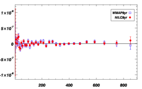
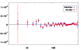
Figure 5: The red filled circles show the cross-angular power spectrum of CMB temperature anisotropies ($T$-mode) and $B$-mode of CMB polarisation estimated using $9$ years of observation of WMAP. The dark blue open squares show the $9$-year angular power spectrum of $E$-mode of CMB polarisation published by the WMAP collaboration. The top panel uses a linear scale in the horizontal axis, and the bottom panel a logarithmic scale.

Table 4: Comparison of our estimate of binned cross-angular power spectrum of CMB temperature anisotropies ($T$-mode) and $B$-mode of CMB polarisation with that provided by WMAP team. The quantities tabulated are $D^{\prime}_{l}=(l+1)C_{l}^{TB}/2\pi$ and $\Delta D^{\prime}_{l}=(l+1)\Delta C_{l}^{TB}/2\pi$.

$l_{\rm range}$	$D_{l}^{\prime,\rm nilc}$	$D_{l}^{\prime,\rm wmap}$	$\Delta D_{l}^{\prime,\rm nilc}$	$\Delta D_{l}^{\prime,\rm wmap}$
	(mK2)	(mK2)	(mK2)	(mK2)
2–7	3.853e-08	2.043e-07	1.084e-06	4.745e-07
8–13	1.366e-07	2.655e-08	1.590e-07	1.757e-07
14–20	1.540e-10	6.373e-08	1.041e-07	1.163e-07
21–24	1.817e-07	5.569e-08	1.169e-07	1.320e-07
25–30	2.142e-07	2.289e-07	8.465e-08	9.887e-08
31–36	-1.212e-07	-4.232e-08	8.199e-08	9.198e-08
37–44	-1.580e-07	-1.707e-07	6.306e-08	7.538e-08
45–52	2.576e-08	-2.907e-08	6.179e-08	7.239e-08
53–60	-7.157e-08	-7.499e-08	6.029e-08	7.070e-08
61–70	8.001e-08	7.028e-08	5.305e-08	6.245e-08
71–81	-4.424e-08	-5.215e-08	4.764e-08	5.947e-08
82–92	-5.287e-08	-5.369e-08	4.680e-08	6.005e-08
93–104	6.241e-08	8.456e-08	4.580e-08	5.856e-08
105–117	-4.843e-08	-1.083e-07	4.419e-08	5.776e-08
118–132	1.908e-08	4.423e-08	4.159e-08	5.557e-08
133–147	-1.114e-08	-2.427e-08	4.142e-08	5.759e-08
148–163	3.772e-08	5.198e-08	4.159e-08	5.768e-08
164–181	-2.657e-08	5.853e-09	4.064e-08	5.613e-08
182–200	5.280e-08	6.994e-08	4.071e-08	5.604e-08
201–220	2.395e-08	7.868e-08	4.072e-08	5.545e-08
221–241	-7.953e-08	-5.467e-08	4.005e-08	5.419e-08
242–265	4.689e-08	6.071e-08	3.742e-08	4.983e-08
266–290	6.394e-08	6.602e-08	3.576e-08	4.688e-08
291–317	-4.613e-08	-4.412e-09	3.317e-08	4.225e-08
318–347	-1.451e-08	-4.799e-08	3.001e-08	3.677e-08
348–379	-2.619e-08	-1.354e-08	2.727e-08	3.286e-08
380–415	-2.188e-09	-5.634e-09	2.593e-08	3.067e-08
416–456	-9.703e-09	4.405e-09	2.803e-08	3.229e-08
457–502	-5.652e-10	1.875e-09	3.297e-08	3.737e-08
503–555	4.714e-08	5.426e-08	3.859e-08	4.410e-08
556–619	6.403e-08	6.695e-08	4.373e-08	4.811e-08
620–698	3.229e-09	3.128e-08	5.358e-08	5.655e-08
699–800	5.605e-08	-1.781e-08	7.684e-08	7.991e-08
801–900	8.951e-08	-5.222e-08	1.308e-07	1.347e-07

4.6.3 $TB$ cross-spectrum

Our result for the $TB$ cross-spectrum, compared to the WMAP collaboration one, is shown in figure 5. Theoretically, this cross-spectrum is supposed to vanish (to preserve the parity symmetry), and significant departure from zero would be the sign of either unknown systematics in the measurement (including residual foregrounds), or new physics. Our measurement is indeed compatible with zero (see table 4).

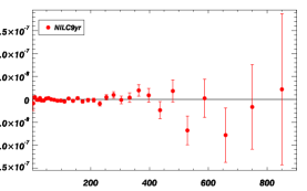
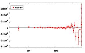
Figure 6: The red filled circles show the cross-angular power spectrum of $E$-mode and $B$-mode of CMB polarisation estimated using $9$ years of observations of WMAP. The top panel uses a linear scale in the horizontal axis, and the bottom panel a logarithmic scale. We use the same legend and color code for data points in this figure as in Figs. 4, 5 and 7, although WMAP data points are absent here.

Table 5: Our estimate of binned cross-angular power spectrum of $E$-mode and $B$-mode of CMB polarisation. The quantities tabulated are $D^{\prime}_{l}=(l+1)C_{l}^{EB}/2\pi$ and $\Delta D^{\prime}_{l}=(l+1)\Delta C_{l}^{EB}/2\pi$.

$l_{\rm range}$	$D_{l}^{\prime,\rm nilc}$	$\Delta D_{l}^{\prime,\rm nilc}$
	(mK2)	(mK2)
2–7	-7.996e-09	1.801e-08
8–13	5.526e-09	3.435e-09
14–20	-2.265e-09	2.968e-09
21–24	-1.599e-09	3.963e-09
25–30	3.589e-09	3.144e-09
31–36	-4.133e-09	3.442e-09
37–44	-3.657e-09	2.950e-09
45–52	1.986e-09	3.303e-09
53–60	2.373e-09	3.512e-09
61–70	-5.980e-10	3.348e-09
71–81	-3.026e-09	3.192e-09
82–92	-6.053e-09	3.350e-09
93–104	-3.207e-09	3.465e-09
105–117	-6.120e-09	3.509e-09
118–132	3.808e-09	3.380e-09
133–147	-5.027e-09	3.490e-09
148–163	1.979e-09	3.771e-09
164–181	-5.674e-09	4.013e-09
182–200	-3.703e-09	4.435e-09
201–220	-3.137e-09	5.006e-09
221–241	-1.110e-08	5.731e-09
242–265	6.418e-09	6.430e-09
266–290	1.163e-08	7.682e-09
291–317	-1.343e-09	9.405e-09
318–347	8.437e-09	1.154e-08
348–379	2.162e-08	1.404e-08
380–415	6.150e-09	1.677e-08
416–456	-3.007e-08	2.081e-08
457–502	2.750e-08	2.683e-08
503–555	-7.581e-08	3.500e-08
556–619	3.258e-09	4.669e-08
620–698	-1.062e-07	6.620e-08
699–800	1.443e-09	1.031e-07
801–900	-1.097e-07	1.842e-07

4.6.4 $EB$ cross-spectrum

The WMAP collaboration has not provided cross-angular power spectra for $E$ and $B$-modes of CMB polarisation. Our estimated $EB$ cross-power spectrum, displayed in figure 6 and tabulated in table 5, is compatible with zero as expected from the current cosmological best-fit model.

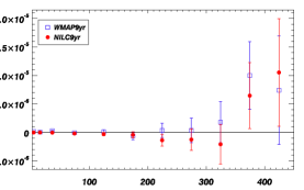
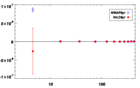
Figure 7: The red filled circles show the angular power spectrum of $B$-mode of CMB polarisation estimated using $9$ years of observations of WMAP. The top panel uses a linear scale in the horizontal axis, and the bottom panels a logarithmic scale. The dark blue open squares show the $9$-year angular power spectrum of $B$-mode of CMB polarisation published by the WMAP collaboration.

Table 6: Comparison of our estimate of binned angular power spectrum of $B$-mode of CMB polarisation, with that provided by WMAP team. The quantities tabulated are $D_{l}=l(l+1)C_{l}^{BB}/2\pi$ and $\Delta D_{l}=l(l+1)\Delta C_{l}^{BB}/2\pi$.

$l_{\rm range}$	$D_{l}^{\rm nilc}$	$D_{l}^{\rm wmap}$	$\Delta D_{l}^{\rm nilc}$	$\Delta D_{l}^{\rm wmap}$
	(mK2)	(mK2)	(mK2)	(mK2)
2–7	-3.748e-08	1.776e-07	1.178e-07	1.683e-08
8–23	-2.005e-09	4.749e-08	4.578e-08	3.290e-08
24–49	-2.914e-08	2.867e-07	9.191e-08	7.243e-08
50–99	-2.457e-07	-5.148e-08	1.647e-07	1.494e-07
100–149	-4.836e-07	1.167e-07	3.302e-07	3.500e-07
150–199	-2.687e-07	-6.025e-07	6.234e-07	6.885e-07
200–249	-1.804e-06	3.528e-07	1.160e-06	1.248e-06
250–299	-1.021e-06	3.532e-07	2.115e-06	2.162e-06
300–349	-2.692e-06	1.793e-06	3.883e-06	3.627e-06
350–399	8.445e-06	9.989e-06	6.468e-06	5.946e-06
400–449	1.545e-05	7.411e-06	1.056e-05	9.517e-06

4.6.5 $BB$ angular power spectrum

Finally, the power spectrum of CMB $B$-modes is of special interest, as it provides one of the most promising means of detecting primordial tensor modes in the early universe, and constrain models of inflation. Significant effort is currently undertaken to prepare the measurement of $B$-modes with a future space mission. One such mission, the Cosmic Origins Explorer (COrE), has been proposed to ESA within Cosmic Vision 2015-2025 (The COrE Collaboration et al., 2011). Missions with similar objectives, but different designs, have been proposed to NASA (see, e.g., Baumann et al., 2009). Contamination by foregrounds is one of the main worries for this measurement, and the investigation of the severeness of the contamination, as well as the development and validation of component separation methods adapted to the challenge of measuring CMB $B$-modes, has focused significant attention recently (Tucci et al., 2005; Stivoli et al., 2006; Amblard, Cooray, & Kaplinghat, 2007; Betoule et al., 2009; Dunkley et al., 2009; Efstathiou, Gratton, & Paci, 2009; Stivoli et al., 2010).

Clearly, the WMAP mission lacks the sensitivity to place a strong limit on the $B$-mode polarisation. While our result does not show any detection of $B$-modes (see figure 7 and table 6), one of the points provided by the WMAP collaboration, in the first multipole bin, is significantly discrepant.

It is difficult for us to comment on the origin of this discrepancy, as we do not exactly know how the WMAP error bars are obtained. It may be that the WMAP data points published on the LAMBDA website neglects noise correlations, or possible residual systematics or foregrounds. The exact meaning of the posted error bars should probably be clarified by the WMAP team. Our estimated error bar, based solely on the dispersion of the data points used to generate the binned power spectrum, seems to be more robust in that respect.

We are confident that our method, which has been also tested on realistic simulations, is more effective for reducing foregrounds than simple masking or template decorrelation. On simulations of future observations with COrE, we have shown that it allows to reject foreground contamination effectively enough to measure tensor to scalar ratio of $10^{-3}$, limited by the sensitivity of the observations rather than foreground contamination.

5 Goodness of fit values

Finally, in order to demonstrate how well our measurements fit with WMAP $9$-year best-fit $\Lambda CDM$ model, we have computed reduced $\chi^{2}$ values to estimate the goodness of fit of our estimates per multipole bin for each angular power spectrum. In principle a value of goodness of fit per multipole bin equal to unity indicates that the extent of the match between observations and estimates is in agreement with the error variance. Table 7 shows good compatibility of our measured spectra with the best-fit cosmological model. The goodness of fit values shown in the first two columns of this table are obtained from the measured CMB power spectra and their errors for all multipoles under consideration. However, the CMB likelihood is non-Gaussian at large angular scales and hence, the use of simple $\chi^{2}$ statistics is sub-optimal at such low multipoles. Hence, the goodness of fit values, obtained from the same measured power spectra and their errors for multipoles greater than $23$, are tabulated in the last two columns of table 7 for comparison. In either case, our measurement of $EE$ and $BB$ spectra is in significantly better agreement with the WMAP best-fit model than that provided by WMAP collaboration, while $TE$ and $TB$ are marginally discrepant with the WMAP best fit model, with a reduced $\chi^{2}$ of order $1.4$ for $34$ degrees of freedom (due in particular to a few points several sigmas away between $l=10$ and $40$). A complete investigation of this requires a more accurate model of the measurement, and in particular of correlated errors, and is beyond the scope of the present paper.

Table 7: Comparison of goodness of fit values per multipole bin

$XY$	$NILC$	$WMAP$	$NILC$	$WMAP$
	(all $l$)	(all $l$)	($l>23$)	($l>23$)
$EE$	0.86	2.21	0.87	1.81
$BB$	0.82	12.16	0.99	2.27
$TE$	1.48	0.94	1.58	0.83
$TB$	1.38	1.08	1.45	1.20
$EB$	0.95	$--$	0.99	$--$

6 Conclusions

In this work, we have computed CMB power spectra for polarised WMAP observations. CMB polarisation maps are obtained from WMAP observations using linear combinations that minimise the variance of the recovered CMB on spherical wavelet (needlet) domains, that are subsequently used to compute CMB power spectra.

Our analysis differs substantially from that of the WMAP team: we use all WMAP channels, use a needlet ILC over the full range of harmonic modes, and produce $9$ independent maps for each of $T$, $E$ and $B$, from the different years of observation. Our estimated error bars do not rely on a model of the WMAP noise, but instead are computed directly from the estimated same-year power spectra ($9$ in our case) and cross-year power spectra ($36$ in case of $EE$ and $BB$ spectra, and $72$ in case $TE$, $TB$ and $EB$ spectra).

We find that our $EE$ power spectrum is in excellent agreement with the expectations from the current cosmological model, while the $9$-year WMAP $EE$ spectrum available publicly on the Lambda web site seems to be systematically higher. Similarly, on very large scale, our $BB$ power spectrum is consistent with zero, while the $9$-year WMAP $BB$ spectrum in first multipole bin is not compatible with zero.

The agreement of our $TE$ and $TB$ measurements with the WMAP ones and with the theoretical best fit model are good, but not perfect. The origin of the discrepancy is not fully understood. Finally, our measurements of the $EB$ spectra are compatible with zero, as expected for a standard cosmological model.

Appendix

Suppose we have $M$ measurements (one measurement per year of observation) of the full sky CMB, such that each of these measurements contains the same signal which comprises the true CMB and residuals of foreground emission and noise. The (residual) noise in these measurements is statistically independent from year to year. The harmonic coefficients of these measurements are expressed as,

$$A^{X,I}_{lm}=S^{X}_{lm}+N^{X,I}_{lm}\hskip 14.45377ptX=\{T,E,B\}\hskip 14.45377ptI=1,..,M.$$ (27)

Here $A^{X}_{lm}$, $S^{X}_{lm}$ and $N^{X}_{lm}$ are the harmonic coefficients of the measured CMB, of the sum of true CMB and residual foreground, and of residual noise respectively. Since signal and residual noise, and residual noise from year to year, are statically independent, they obey the following relations,

$$E\left[S^{X}_{lm}N^{Y,I*}_{l^{\prime}m^{\prime}}\right]=0$$ (28)

$$E\left[S^{X}_{lm}S^{Y*}_{l^{\prime}m^{\prime}}\right]=S^{XY}_{l}\delta_{ll^{\prime}}\delta_{mm^{\prime}}$$ (29)

$$E\left[N^{X,I}_{lm}N^{Y,J*}_{l^{\prime}m^{\prime}}\right]=N^{XY}_{l}\delta_{ll^{\prime}}\delta_{mm^{\prime}}\delta_{IJ}$$ (30)

where, $S^{XY}_{l}$ and $N^{XY}_{l}$ are the angular power spectra of signal and residual noise respectively.

From these $M$ maps $A^{X,I}_{lm}$, we have $M(M-1)$ cross-year measurements $(\widehat{C}^{XY,IJ},I\neq J)$ of the angular power spectrum, such that each of them is an unbiased estimator of $S^{XY}_{l}$ (although they are not independent). We have:

$$\widehat{C}^{XY,IJ}_{l}=\frac{1}{2l+1}\sum^{l}_{m=-l}A^{X,I}_{lm}A^{Y,J*}_{lm}$$ (31)

$$E\left[\widehat{C}^{XY,IJ}_{l}\right]=S^{XY}_{l}+N^{XY}_{l}\delta_{IJ}.$$ (32)

The average of all cross-year measurements of angular power spectra is also an unbiased estimator of signal power spectrum $S^{XY}_{l}$:

$$\widehat{C}^{XY}_{l}=\frac{1}{M(M-1)}\sum^{M}_{I,J=1}\widehat{C}^{XY,IJ}_{l}(1-\delta_{IJ})$$ (33)

The variance of $\widehat{C}^{XY}_{l}$ is, by definition,

$$V^{XY}_{l}=E\left[\left(\widehat{C}^{XY}_{l}\right)^{2}\right]-\left(E\left[\widehat{C}^{XY}_{l}\right]\right)^{2}$$ (34)

where, $E\left[\widehat{C}^{XY}_{l}\right]$ and $E\left[\left(\widehat{C}^{XY}_{l}\right)^{2}\right]$ are the expectation values of $\widehat{C}^{XY}_{l}$ and $\left(\widehat{C}^{XY}_{l}\right)^{2}$ respectively. We have:

$$E\left[\widehat{C}^{XY}_{l}\right]=\frac{1}{M(M-1)}\sum^{M}_{I,J=1}E\left[\widehat{C}^{XY,IJ}_{l}\right](1-\delta_{IJ})=S^{XY}_{l}$$ (35)

and

$$E\left[\left(\widehat{C}^{XY}_{l}\right)^{2}\right]=\left[\frac{1}{M(M-1)}\right]^{2}\sum^{M}_{\begin{subarray}{c}I,J,\\ K,L=1\end{subarray}} E\left[\widehat{C}^{XY,IJ}_{l}\widehat{C}^{XY,KL}_{l}\right]$$

$$\times(1-\delta_{IJ})(1-\delta_{KL})$$ (36)

In order to express $E\left[\left(\widehat{C}^{XY}_{l}\right)^{2}\right]$ in terms of $S^{XY}_{l}$ and $N^{XY}_{l}$, first we express the expectation value of correlations among $(\widehat{C}^{XY,IJ})$ in terms of $S^{XY}_{l}$ and $N^{XY}_{l}$. We get:

$$E\left[\widehat{C}^{XY,IJ}_{l}\widehat{C}^{XY,KL}_{l}\right]=\left(S^{XY}_{l}\right)^{2}$$

$$+ \frac{1}{2l+1}\left[\left\{\left(S^{XY}_{l}\right)^{2}+S^{XX}_{l}S^{YY}_{l}\right\}+\left(S^{XX}_{l}N^{YY}_{l}\delta_{JL}\right.\right.$$

$$+ \left.\left.S^{YY}_{l}N^{XX}_{l}\delta_{IK}+S^{XY}_{l}N^{XY}_{l}\delta_{IJ}+S^{XY}_{l}N^{XY}_{l}\delta_{KL}\right)\right.$$

$$+ \left.\left\{\left(N^{XY}_{l}\right)^{2}\delta_{IL}\delta_{JK}+N^{XX}_{l}N^{YY}_{l}\delta_{IK}\delta_{JL}\right\}\right].$$ (37)

Then, we express $E\left[\left(\widehat{C}^{XY}_{l}\right)^{2}\right]$ in terms of $S^{XY}_{l}$ and $N^{XY}_{l}$ by combining equations 36 and 37,

$$E\left[\left(\widehat{C}^{XY}_{l}\right)^{2}\right]$$

$$=\left(S^{XY}_{l}\right)^{2}+ \frac{1}{2l+1}\left[\left\{\left(S^{XY}_{l}\right)^{2}+S^{XX}_{l}S^{YY}_{l}\right\}\right.\hskip 36.135pt$$

$$+ \left.\frac{1}{M}\left(S^{XX}_{l}N^{YY}_{l}+S^{YY}_{l}N^{XX}_{l}+2\,S^{XY}_{l}N^{XY}_{l}\right)\right.$$

$$+ \left.\frac{1}{M(M-1)}\left\{\left(N^{XY}_{l}\right)^{2}+N^{XX}_{l}N^{YY}_{l}\right\}\right].$$ (38)

Finally, we express $V^{XY}_{l}$ in terms of signal and noise power spectra, by combining equations 34, 35 and 38.

$$V^{XY}_{l}= \frac{1}{2l+1}\left[\left\{\left(S^{XY}_{l}\right)^{2}+S^{XX}_{l}S^{YY}_{l}\right\}\right.\hskip 72.26999pt$$

$$\hskip 14.45377pt+\left.\frac{1}{M}\left(S^{XX}_{l}N^{YY}_{l}+S^{YY}_{l}N^{XX}_{l}+2\,S^{XY}_{l}N^{XY}_{l}\right)\right.$$

$$\hskip 14.45377pt+\left.\frac{1}{M(M-1)}\left\{\left(N^{XY}_{l}\right)^{2}+N^{XX}_{l}N^{YY}_{l}\right\}\right].$$ (39)

In order to define an estimator for $V^{XY}_{l}$, first we define an estimator $(\widehat{N}^{XY}_{l})$ for the residual noise power spectrum $N^{XY}_{l}$.

$$\widehat{N}^{XY}_{l} =\frac{1}{M}\sum^{M}_{I=1}\widehat{C}^{XY,II}_{l}-\widehat{C}^{XY}_{l}$$

$$=\frac{1}{M}\sum^{M}_{I=1}\widehat{C}^{XY,II}_{l}-\frac{1}{M(M-1)}\sum^{M}_{I,J=1}\widehat{C}^{XY,IJ}_{l}(1-\delta_{IJ}).$$ (40)

In equation 40, the first term is an unbiased estimator of the sum of the angular power spectra of signal and residual noise, and the second term an unbiased estimator of the angular power spectra of signal only.

Then, the estimator for $V^{XY}_{l}$ is constructed by replacing $S_{l}$ and $N_{l}$ with the best-fit theoretical power spectrum $C_{l,\rm th}$ and the estimated noise power spectrum $\widehat{N}_{l}$ respectively in equation 39.

$$\widehat{V}^{XY}_{l} =\frac{1}{2l+1}\left[\left\{\left(C^{XY}_{l,\rm th}\right)^{2}+C^{XX}_{l,\rm th}C^{YY}_{l,\rm th}\right\}\right.$$

$$+\left.\frac{1}{M}\left(C^{XX}_{l,\rm th}\widehat{N}^{YY}_{l}+C^{YY}_{l,\rm th}\widehat{N}^{XX}_{l}+2\,C^{XY}_{l,\rm th}\widehat{N}^{XY}_{l}\right)\right.$$

$$+\left.\frac{1}{M(M-1)}\left\{\left(\widehat{N}^{XY}_{l}\right)^{2}+\widehat{N}^{XX}_{l}\widehat{N}^{YY}_{l}\right\}\right].$$ (41)

In practice, the auto and cross angular power spectra are obtained from observed NILC CMB maps after applying a mask. These angular power spectra are corrected for the mask using the MASTER method (Hivon et al., 2002) before using them to measure residual noise power spectra. The estimated variance is divided by the sky fraction $f_{\rm sky}$, as the effective number of modes for an arbitrary multipole $l$, is now $(2l+1)f_{\rm sky}$ instead of $(2l+1)$ (even if residual noise power spectra is corrected for the mask).

$f_{\rm sky}$ is estimated as the average value of the product of the two masks used, e.g. for $\widehat{C}^{TX}_{l}$ ($X$ being $E$ or $B$) we use:

$$f_{\rm sky}=\frac{1}{4\pi}\int m_{T}(\hat{n})\,m_{P}(\hat{n})\,d\Omega,$$ (42)

where $m_{T}(\hat{n})$ and $m_{P}(\hat{n})$ are the masks for the temperature and polarisation respectively (including noise weighting modulation when necessary, i.e., for the noise-weighted estimates the masks are real-valued, not just binary masks). For $\widehat{C}^{XY}_{l}$ ($X$ and $Y$ being each either $E$ or $B$) we use:

$$f_{\rm sky}=\frac{1}{4\pi}\int\left[m_{P}(\hat{n})\right]^{2}\,d\Omega.$$ (43)

References

- Amblard, Cooray, & Kaplinghat (2007) Amblard A., Cooray A., Kaplinghat M., 2007, PhRvD, 75, 083508.
- Astier et al. (2006) Astier P., et al., 2006, A&A, 447, 31
- Baker et al. (1999) Baker J. C., et al., 1999, MNRAS, 308, 1173
- Basak & Delabrouille (2012) Basak S., Delabrouille J., 2012, MNRAS, 419, 1163
- Baumann et al. (2009) Baumann et al. (CMBPol Study Team), AIP Conf.Proc. 1141, 10 (2009), 0811.3919
- Bennett et al. (1992) Bennett C. L., et al., 1992, ApJ, 396, L7
- Bennett et al. (1996) Bennett C. L., et al., 1996, ApJ, 464, L1
- Bennett et al. (2003) Bennett C. L., et al., 2003, ApJS, 148, 1
- Benoît et al. (2003a) Benoît A., et al., 2003, A&A, 399, L19
- Benoît et al. (2003b) Benoît A., et al., 2003, A&A, 399, L25
- Benoît et al. (2004) Benoît A., et al., 2004, A&A, 424, 571
- Betoule et al. (2009) Betoule M., Pierpaoli E., Delabrouille J., Le Jeune M., Cardoso J.-F., 2009, A&A, 503, 691
- Bischoff et al. (2008) Bischoff C., et al., 2008, ApJ, 684, 771
- Brown et al. (2009) Brown M. L., et al., 2009, ApJ, 705, 978
- Cardoso et al. (2008) Cardoso, J.-F., Le Jeune, M., Delabrouille, J., Betoule, M., & Patanchon, G. 2008, IEEE Journal of Selected Topics in Signal Processing, 2, 735
- Chiang et al. (2010) Chiang H. C., et al., 2010, ApJ, 711, 1123
- The COrE Collaboration et al. (2011) The COrE Collaboration, et al., 2011, arXiv:1102.2181
- Das et al. (2011a) Das S., et al., 2011, ApJ, 729, 62
- Das et al. (2011b) Das S., et al., 2011, PhRvL, 107, 021301
- de Bernardis et al. (2000) de Bernardis P., et al., 2000, Nature, 404, 955
- Delabrouille et al. (2003) Delabrouille, J., Cardoso, J.-F., & Patanchon, G. 2003, MNRAS, 346, 1089
- Delabrouille & Cardoso (2009) Delabrouille J., Cardoso J.-F., 2009, LNP, 665, 159
- Delabrouille et al. (2009) Delabrouille J., Cardoso J.-F., Le Jeune M., Betoule M., Faÿ G., Guilloux F., 2009, A&A, 493, 835
- Delabrouille et al. (2012) Delabrouille J. et al., 2012, arXiv:1207.3675
- Dick, Remazeilles, & Delabrouille (2010) Dick J., Remazeilles M., Delabrouille J., 2010, MNRAS, 401, 1602
- Dickinson et al. (2004) Dickinson C., et al., 2004, MNRAS, 353, 732
- Dunkley et al. (2009) Dunkley J., et al., 2009, AIPC, 1141, 222
- Efstathiou, Gratton, & Paci (2009) Efstathiou G., Gratton S., Paci F., 2009, MNRAS, 397, 1355
- Eisenstein et al. (2005) Eisenstein D. J., et al., 2005, ApJ, 633, 560
- Eriksen et al. (2004) Eriksen H. K., Banday A. J., Górski K. M., Lilje P. B., 2004, ApJ, 612, 633
- Faÿ et al. (2008) Faÿ G., Guilloux F., Betoule M., Cardoso J.-F., Delabrouille J., Le Jeune M., 2008, PhRvD, 78, 083013
- Finkbeiner (2003) Finkbeiner D. P., 2003, ApJS, 146, 407
- Freedman et al. (2001) Freedman W. L., et al., 2001, ApJ, 553, 47
- Goldberg et al. (1967) Goldberg J. N., Macfarlane A. J., Newman E. T., Rohrlich F., Sudarshan E. C. G., 1967, JMP, 8, 2155
- Górski et al. (2005) Górski K. M., Hivon E., Banday A. J., Wandelt B. D., Hansen F. K., Reinecke M., Bartelmann M., 2005, ApJ, 622, 759
- Guilloux, Faÿ, & Cardoso (2009) Guilloux F., Faÿ G., Cardoso J.-F., 2009, Appl. Comput. Harmon. Anal., 26, vol. 2, 143
- Guy et al. (2010) Guy J., et al., 2010, A&A, 523, A7
- Hanany et al. (2000) Hanany S., et al., 2000, ApJ, 545, L5
- Haslam et al. (1981) Haslam C. G. T., Klein U., Salter C. J., Stoffel H., Wilson W. E., Cleary M. N., Cooke D. J., Thomasson P., 1981, A&A, 100, 209
- Hinshaw et al. (2013) Hinshaw G. et al., 2012, arXiv:1212.5226
- Hivon et al. (2002) Hivon, E., Górski, K. M. and Netterfield, C. B. and Crill, B. P. and Prunet, S. and Hansen, F., 2002, ApJ, 567, 2
- Hu, Hedman, & Zaldarriaga (2003) Hu W., Hedman M. M., Zaldarriaga M., 2003, PhRvD, 67, 043004
- Kamionkowski, Kosowsky, & Stebbins (1997) Kamionkowski M., Kosowsky A., Stebbins A., 1997, PhRvD, 55, 7368
- Kaplan & Delabrouille (2002) Kaplan J., Delabrouille J., 2002, AIPC, 609, 209
- Keisler et al. (2011) Keisler R., et al., 2011, ApJ, 743, 28
- Larson et al. (2011) Larson D., et al., 2011, ApJS, 192, 16
- Leitch et al. (2005) Leitch E. M., Kovac J. M., Halverson N. W., Carlstrom J. E., Pryke C., Smith M. W. E., 2005, ApJ, 624, 10
- Marinucci et al. (2008) Marinucci D., et al., 2008, MNRAS, 383, 539
- Montroy et al. (2006) Montroy T. E., et al., 2006, ApJ, 647, 813
- Narcowich, Petrushev & Ward (2006) Narcowich, F. Petrushev, P. and Ward, J., 2006, SIAM J. Math. Anal. 38, vol. 2, 574
- Nolta et al. (2009) Nolta M. R., et al., 2009, ApJS, 180, 296
- Pearson et al. (2003) Pearson T. J., et al., 2003, ApJ, 591, 556
- Perlmutter et al. (1999) Perlmutter S., et al., 1999, ApJ, 517, 565
- Piacentini et al. (2006) Piacentini F., et al., 2006, ApJ, 647, 833
- Pietrobon et al. (2008) Pietrobon D., Amblard A., Balbi A., Cabella P., Cooray A., Marinucci D., 2008, PhRvD, 78, 103504
- Planck collaboration XV (2013) Planck collaboration XV, 2013, submitted to A&A, arXiv:1303.5075
- Planck Collaboration XVI (2013) Planck Collaboration XVI, 2013, submitted to A&A, arXiv:1303.5076
- Pryke et al. (2009) Pryke C., et al., 2009, ApJ, 692, 1247
- QUIET Collaboration et al. (2011) QUIET Collaboration, et al., 2011, ApJ, 741, 111
- Rebolo et al. (2004) Rebolo R., et al., 2004, MNRAS, 353, 747
- Rees (1968) Rees M. J., 1968, ApJ, 153, L1
- Reichardt et al. (2009) Reichardt C. L., et al., 2009, ApJ, 694, 1200
- Rosset et al. (2007) Rosset C., Yurchenko V. B., Delabrouille J., Kaplan J., Giraud-Héraud Y., Lamarre J.-M., Murphy J. A., 2007, A&A, 464, 405
- Rudjord et al. (2009) Rudjord Ø., Hansen F. K., Lan X., Liguori M., Marinucci D., Matarrese S., 2009, ApJ, 701, 369
- Saha (2011) Saha, R., 2011, ApJL, 739, L56
- Saha, Jain & Souradeep (2006) Saha R., Jain P., Souradeep T., 2006, ApJ, 645, L89
- Saha, Prunet, Jain & Souradeep (2008) Saha R., Prunet S., Jain P., Souradeep T., 2008, PhRvD, 78, 023003
- Samal, Saha, Delabrouille, Prunet, Jain & Souradeep (2010) Samal P. K., Saha R., Delabrouille J., Prunet S., Jain P., Souradeep T., 2010,. ApJ, 714, 840
- Schlegel, Finkbeiner, & Davis (1998) Schlegel D. J., Finkbeiner D. P., Davis M., 1998, ApJ, 500, 525
- Seljak, Slosar, & McDonald (2006) Seljak U., Slosar A., McDonald P., 2006, JCAP, 10, 14
- Sievers et al. (2007) Sievers J. L., et al., 2007, ApJ, 660, 976
- Stivoli et al. (2006) Stivoli F., Baccigalupi C., Maino D., Stompor R., 2006, MNRAS, 372, 615
- Souradeep (2011) Souradeep T., 2011, Bull. Astron. Soc. India, 39, 163
- Souradeep, Saha., Jain (2006) Souradeep T., Saha R., Jain P., 2006, Nat, 50, 854
- Stivoli et al. (2010) Stivoli F., Grain J., Leach S. M., Tristram M., Baccigalupi C., Stompor R., 2010, MNRAS, 408, 2319
- Tegmark (1998) Tegmark M., 1998, ApJ, 502, 1
- Tegmark, de Oliveira-Costa, & Hamilton (2003) Tegmark, M., de Oliveira-Costa, A., Hamilton, A. J. S., PhRvD 68 (2003), 123523
- Tucci et al. (2005) Tucci M., Martínez-González E., Vielva P., Delabrouille J., 2005, MNRAS, 360, 935
- Wu et al. (2007) Wu J. H. P., et al., 2007, ApJ, 665, 55
- Zaldarriaga & Seljak (1997) Zaldarriaga M., Seljak U., 1997, PhRvD, 55, 1830