Kosterlitz-Thouless transition in disordered two-dimensional topological insulators

Abstract

The disorder-driven metal-insulator transition in the quantum spin Hall systems is studied by scaling analysis of the Thouless conductance $g$. Below a critical disorder strength, the conductance is independent of the sample size $M$, an indication of critically delocalized electron states. The calculated beta function $\beta=d\ln g/d\ln M$ indicates that the metal-insulator transition is Kosterlitz-Thouless (KT) type, which is characterized by bounding and unbounding of vortex-antivortex pairs of the local currents. The KT like metal-insulator transition is a basic characteristic of the quantum spin Hall state, being independent of the time-reversal symmetry.

The Kosterlitz-Thouless (KT) transition, which was first proposed by Kosterlitz and Thouless in two-dimensional (2D) XY model, KT1 is an important phenomenon in 2D systems, such as 2D magnets, superconductors and superfluids in thin films. It is a typical topological phase transition, which has been understood as bounding and unbounding of vortex-antivortex pairs. KT1 ; KT3 In recent years, the KT like transition was also found in 2D disordered electronic models, including the model with random magnetic fluxes, Ktfordisorder1 ; Ktfordisorder2 and the graphene model with long-range impurity scattering potential. Xie These systems show localization-delocalization transitions with decreasing disorder strength. On the metallic side, the Thouless conductance $g$ is independent of the system size $M$, leading to a vanishing beta function Scaling ; beta defined as $\beta=d\ln g/d\ln M$, which is an essential characteristic of the KT transition. Ktfordisorder1 ; Ktfordisorder2 ; Xie From the classification scheme based on the universality classes, Review1 the former model Ktfordisorder1 ; Ktfordisorder2 belongs to the unitary class, and the existence of delocalized states is due to the random phases in the hopping integrals, which result in the Chern number fluctuations. DNShengRF The latter model Xie belongs to the orthogonal class, and the electron delocalization arises from the nonzero Berry phases at two Dirac points, which cannot annihilate each other when the impurity scattering is long-range correlated.

A topological insulator KaneR ; ZhangR2 is a band insulator with gapless edge states or surface states traversing the band gap, which originate from the nontrivial band topology. The gapless nature of the edge states or surface states is protected by the time-reversal symmetry. The 2D version of the topological insulators, which is also called the quantum spin Hall (QSH) state, was predicted by Kane and Mele Pre1 to exist in a graphene model with intrinsic spin-orbit coupling. Later it was experimentally realized in mercury telluride (HgTe) quantum wells. Exp1 The robustness of the QSH state is associated with new types of topological invariants of the bulk energy bands. Z2 ; Spinchern ; cz ; Prodan1

Since topological invariants are carried by bulk extended states, there have being strong interest in the delocalization problem in the QSH systems. Onoda $et$ $al.$ Nagaosa studied the Kane-Mele model using the transfer matrix method and showed the existence of extended states in a finite energy region in the presence of time reversal symmetry. Based upon calculations of the critical exponents, they suggested that the QSH state belongs to a new universality class different from the ordinary symplectic universality class. symplectic Consistent result was obtained by Prodan using the level statistics analysis. ProdanLevel Employing a continuum model, Mong $et$ $al.$ Mong showed that the surface states of a weak topological insulator with even number of Dirac cores are delocalized in the absence of a mass term, and localization occurs when the mass term and strong disorder are present. This conclusion may also be applicable to the QSH systems. Xu $et$ $al.$ Xu demonstrated numerically that the metallic state in the QSH systems remains to be robust even when the time-reversal symmetry is broken, in glaring contrast to trivial unitary class, where all electron states are localized. This result was attributed to the fact that the nontrivial band topology, as described by the spin Chern numbers, is intact when the time-reversal symmetry is broken. Prodan1 ; Yang The existence of delocalized states in the QSH systems is affirmative, but the basic characteristics of the metal-insulator transition have not been well established.

In this Letter, from calculations of the Thouless conductance in the Kane-Mele model, it is shown that the disorder-driven metal-insulator transition in the QSH system is a KT phase transition. Below a critical disorder strength, the Thouless conductance $g$ is found to be independent of the sample size, an indication of critically delocalized electron states. The beta function obtained from the universal scaling function of the conductance, vanishes in the metallic phase. Through mapping the local currents onto the local spins in the 2D $XY$ model, we further show that the KT transition is characterized by bounding and unbounding of vortex-antivortex pairs. The KT like metal-insulator transition is a fundamental characteristic of the QSH state, allowing to be examined experimentally, which neither depends on the time-reversal symmetry, nor requires any long-range correlations of the disorder.

We start from the Kane-Mele model defined on a 2D honeycomb lattice, Pre1 ; Spinchern ; disorder with the Hamiltonian given by

$$H=-t\sum\limits_{\langle ij\rangle}{c_{i}^{\dagger}{c_{j}}}+\frac{{2i}}{{\sqrt{3}}}{V_{\mbox{\tiny SO}}}\sum\limits_{\langle\langle ij\rangle\rangle}{c_{i}^{\dagger}\overset{\lower 5.0pt\hbox{$\smash{\scriptscriptstyle\rightharpoonup}$}}{\sigma}\cdot({{\overset{\lower 5.0pt\hbox{$\smash{\scriptscriptstyle\rightharpoonup}$}}{d}}_{kj}}\times{{\overset{\lower 5.0pt\hbox{$\smash{\scriptscriptstyle\rightharpoonup}$}}{d}}_{ik}}){c_{j}}}$$

$$+i{V_{\mbox{\tiny R}}}\sum\limits_{\langle ij\rangle}{c_{i}^{\dagger}\hat{\mbox{e}}_{z}\cdot(\overset{\lower 5.0pt\hbox{$\smash{\scriptscriptstyle\rightharpoonup}$}}{\sigma}\times{{\overset{\lower 5.0pt\hbox{$\smash{\scriptscriptstyle\rightharpoonup}$}}{d}}_{ij}}){c_{j}}}+\sum\limits_{i}{{w_{i}}{c_{i}}^{\dagger}}{c_{i}}\ .$$ (1)

Here, the first term is the usual nearest neighbor hopping term with $c_{i}^{\dagger}=(c_{i\uparrow}^{\dagger},c_{i\downarrow}^{\dagger})$ as the electron creation operator on site $i$. The second term is the intrinsic spin-orbit coupling with coupling strength $V_{\mbox{\tiny SO}}$, where $\vec{\sigma}$ are the Pauli matrices, $i$ and $j$ are two next nearest neighbor sites, $k$ is their unique common nearest neighbor, and vector $\vec{d}_{ik}$ points from $k$ to $i$. The third term stands for the Rashba spin-orbit coupling with coupling strength $V_{\mbox{\tiny R}}$. ${w_{i}}$ is a random on-site energy potential uniformly distributed between $\left[-W/2,W/2\right]$, which accounts for nonmagnetic disorder. For convenience, we will set $\hbar$, $t$ and the distance between the nearest neighbor sites all to be unity. In the following calculations, $V_{\mbox{\tiny SO}}=V_{\mbox{\tiny R}}=0.1$ is fixed, so that the model is inside the QSH phase at $W=0$.

The localization property of an infinite 2D system can be extracted from the scaling analysis of the dimensionless Thouless conductance calculated for finite-size samples. Scaling ; beta We consider a rectangular sample with two zigzag sides and two armchair sides. Each zigzag side has $M$ atoms and each armchair side has $2M$ atoms, so that the sample has totally $M\times M$ atoms. The rectangular sample is connected to two semi-infinite leads of the same width with armchair interfaces. At zero temperature, the two-terminal dimensionless Landauer conductance $g_{\mbox{\tiny L}}$ is calculated from the Landauer-Büttiker formula Landauer ${g_{\mbox{\tiny L}}}=\mbox{Tr}[\Gamma_{\mbox{\tiny L}}G^{r}\Gamma_{\mbox{\tiny R}}G^{a}]$, where $G^{r(a)}(E)$ is the retarded (advanced) Green’s function and $\Gamma_{\mbox{\tiny L(R)}}(E)$ is the coupling matrix between the sample and the left (right) lead. The Thouless conductance $g$ is related to the Landauer conductance $g_{L}$ through the relation $1/g=1/{g_{\mbox{\tiny L}}}-1/{N_{\mbox{\tiny C}}}$, Xie ; Braun where $1/N_{\mbox{\tiny C}}$ is the contact resistance between the leads and the sample with $N_{\mbox{\tiny C}}$ as the number of propagating channels in the leads at the Fermi energy $E$.

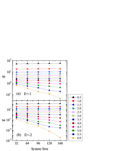
Figure 1: (Color online) Conductance as a function of system size $M$ at $E=-1$ (a) and $E=-2$ (b). Symbols with different colors and shapes correspond to different disorder strengths $W$.

Figure 1 shows the size dependence of the calculated conductance $g$ in logarithmic scale for different disorder strengths $W$ at $E=-1$ and $-2$. Periodic boundary conditions are employed in the transverse direction, so that no contribution from edge states is involved. At given values of $W$ and $M$, the conductance is averaged over 200 to 500 random disorder configurations. Symbols with different shapes are used to distinguish data for different $W$. It is found that the conductance behaves differently with changing sample size in weak and strong disorder regions. For weak disorder, $g$ neither decreases nor increases with increasing sample size. As a result, the conductance is expected to remain constant in the thermodynamic limit, suggesting that the electron states at the Fermi energy are critically delocalized. For strong disorder, $g$ decreases with increasing sample size, corresponding to localized states. A metal-insulator transition occurs at an intermediate critical disorder strength.

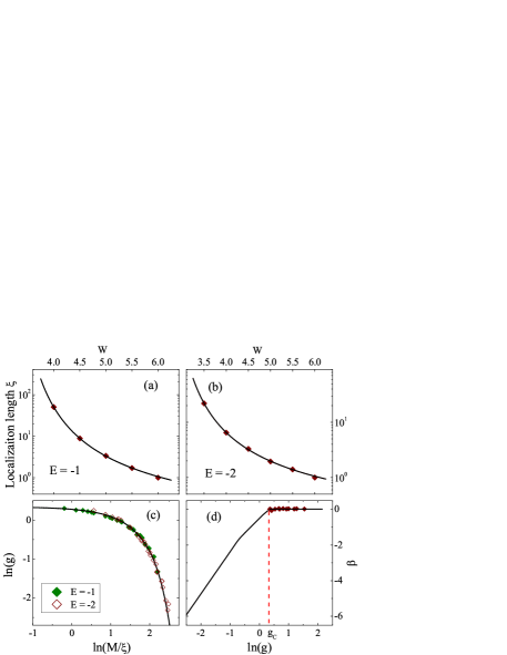
Figure 2: (Color online) (a,b) Calculated localization length $\xi$ (symbols), fitted with an exponential function (solid lines). (c) Universal scaling function $g=f(M/\xi)$, where solid and open symbols are conductance at $E=-1$ and $-2$, respectively, and the solid line represents a smooth functional fit to the data. (d) Calculated beta function.

To further investigate the nature of the metal-insulator phase transition, we perform scaling analysis on the data shown in Fig. 1 and calculate the beta function $\beta=d\ln g/d\ln M$. According to the one-parameter scaling theory, Scaling ; beta the localization length in the thermodynamic limit can be extracted by fitting all the data on the insulator side in Fig. 1 into a universal function $g=f(M/\xi)$, where the fitting parameter $\xi$ yields the localization length in the thermodynamic limit. The obtained localization lengths for $E=-1$ and $-2$ are plotted in Figs. 2a and 2b, respectively, and the universal scaling function $g=f(M/\xi)$ is shown in Fig. 2c. In the above scaling procedure, only the relative magnitudes of the localization lengths $\xi$ can be determined. Therefore, we set $\xi$ at $W=6.0$ to be unity, and the localization lengths for other $W$ are the relative values with respect to it. It is found that the localization length $\xi$ as a function of disorder strength $W$ shown in Figs. 2(a,b) can be fitted with an exponential function $\xi\propto e^{\alpha/\sqrt{W-{W_{\mbox{\tiny C}}}}}$ with $\alpha$ and $W_{\mbox{\tiny C}}$ as two fitting parameters. This behavior indicates an exponential decay of the localization length with increasing the disorder strength in the insulating phase, which is typical of a KT phase transition. KT1 ; KT3 The critical disorder strength for such a metal-insulator transition is obtained as $W_{\mbox{\tiny C}}=3.12$ at $E=-1$ and 2.54 at $E=-2$, respectively. To facilitate the calculation of the beta function $\beta=d\ln g/d\ln M$, we fit the data in Fig. 2c with a smooth function, as indicated by the solid line, which is explained below. In the region of small $\ln(M/\xi)$, the data is fitted with $g=g_{\mbox{\tiny C}}{e^{-(M/\xi)^{1/\nu}}}$, which is consistent with the general behavior of the beta function, $\beta=\frac{1}{\nu}\ln(g/{g_{\mbox{\tiny C}}})$, in the quantum critical region. DNSheng On the other hand, a polynomial fit is used in the region of relatively large $\ln(M/\xi)$. At the boundary between the two regions, $\ln g$ and its derivative $\beta$ are required to be continuous.

After obtaining the smooth fitting function describing the scaling relation between $\ln g$ and $\ln M$, we take its derivative to calculate the beta function $\beta=d\ln g/d\ln M$, as plotted in Fig. 2d. Here, we note that for weak disorder ($W<W_{\mbox{\tiny C}}$), where the conductance is nearly independent of the sample size, the localization length diverges and cannot be treated with the same scaling procedure as above. Instead, we fit the logarithmic conductance $\ln g$ as a function of $\ln M$ with straight lines, and take their slopes as the values of $\beta$, which are shown by the diamonds in Fig. 2d. We see from Fig. 2d that $\beta$ increases with $\ln g$, and vanishes on average above a critical point ($g>g_{\mbox{\tiny C}}\simeq 1.3$) with negligible fluctuations, indicating clearly that the disorder-driven metal-insulator transition is a KT transition, as observed in other disordered 2D electron systems. Ktfordisorder1 ; Ktfordisorder2 ; Xie The behavior of the beta function also suggests that a minimum (critical) conductivity, $\sigma_{c}=g_{\mbox{\tiny C}}(e^{2}/h)/\sqrt{3}\simeq 0.75(e^{2}/h)$ ($1/\sqrt{3}$ being the aspect ratio), exists for the bulk QSH system.

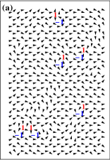
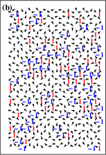
Figure 3: (Color online) Typical distribution of vortices (red positive numbers) and antivortices (blue negative numbers) on the two sides of the KT like transition in a sample with $40\times 40$ sites at $E=-2$ for (a) $W=1.5t$ (metallic phase) and (b) $W=3.5t$ (insulator phase). For clarity, only a part of the sample is shown.

An important characteristic of the traditional KT transition in the $XY$ model is the bounding of vortex-antivortex pairs in the ordered phase near the transition point and unbounding in the disordered phase. KT1 ; KT3 For 2D electron systems, Zhang $et$ $al.$ Xie proposed to map the local currents onto the local spins in the $XY$ model. The bond current vector between sites $m$ and $n$ can be calculated by Xie ; localcurrent1 ; localcurrent3

$${i_{m{\sigma_{2}}\to n{\sigma_{1}}}}=\frac{{-2e}}{\hbar}\int{\frac{{dE}}{{2\pi}}{\mathop{\rm Re}\nolimits}[{H_{m{\sigma_{2}},n{\sigma_{1}}}}G_{n{\sigma_{1}},m{\sigma_{2}}}^{<}(E)]},$$ (2)

where ${\sigma_{1}}$ and ${\sigma_{2}}$ represent the spin index and $G_{n{\sigma_{1}},m{\sigma_{2}}}^{<}(E)$ is the matrix element of the lesser Green’s function. The lesser Green’s function is given by

$${G^{<}}(E)={G^{r}}(E)[i\sum\limits_{\alpha}{{\Gamma_{\alpha}}(E)f_{\alpha}}(E)]{G^{a}}(E)\ ,$$ (3)

where ${f_{\alpha}}(E)={f_{0}}(E+e{V_{\alpha}})$ is the Fermi distribution function in lead $\alpha$ with $V_{\alpha}$ as the electrical potential in the lead. The local current vector defined on site $n$ is ${i_{n}}=\sum_{m{\sigma_{2}}{\sigma_{1}}}{{i_{m{\sigma_{2}}\rightarrow n{\sigma_{1}}}}}$, Xie where the vectorial summation is taken over all the nearest and next nearest neighbors $m$ of site $n$. Along a closed path, the polar angle $\theta_{n}$ of $i_{n}$ is considered to change continuously with changing coordinates, and a topological charge is defined as $c=\frac{1}{2\pi}\oint\nabla\theta\cdot dl$. Xie A nonzero number of $c$ indicates the appearance of a vertex $(c>0)$ or an antivortex $(c<0)$. Figure 3 shows typical distributions of the topological charges on the two sides of the metal-insulator transition. The arrows in the figure indicate only the direction of the local currents, without showing the magnitude for the purpose of visualization. In the delocalized phase (Fig. 3a), a few vortices ($c>0$) and antivortices ($c<0$) are excited in pairs and bounded together, corresponding to the ordered phase at low temperature in the 2D $XY$ model. In the localized phase (Fig. 3b), a large number of vortices and antivortices appear and are mostly unbounded, corresponding to the disordered phase at high temperature.

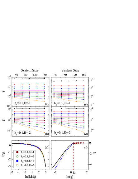
Figure 4: (Color online) (a-d) Conductance as a function of sample size with Fermi energy $E$, in the presence of a vertical Zeeman field $h_{z}$ or a horizontal Zeeman field $h_{x}$. (e) Universal scaling function $g=f(M/\xi)$, where the solid line represents a smooth functional fit to the data. (f) The corresponding beta functions for the time-reversal symmetry broken QSH system (solid line) and time-reversal symmetry invariant QSH system (dotted line).

Finally, we study the effect of breaking the time-reversal symmetry on the KT phase transition, by including a new term $\vec{h}\cdot\vec{\sigma}$ into Hamiltonian (Kosterlitz-Thouless transition in disordered two-dimensional topological insulators), where $\vec{h}$ stands for a uniform Zeeman field. The calculated conductances at $E=-1$ and $-2$ as functions of sample size $M$ for different disorder strengths are shown in Fig. 4(a,b) for a vertical Zeeman field $\vec{h}=(0,0,h_{z}=0.1)$ and in Fig. 4(c,d) for a horizontal field $\vec{h}=(h_{x}=0.1,0,0)$. The parameters are chosen in such a manner that the system is in the time-reversal symmetry broken QSH phase in the clean limit. Yang ; Xu The conductance shown in Fig. 4(a-d) displays similar size dependence to that in Fig. 1. For weak disorder, the conductance is nearly independent of sample size, indicating the existence of the critically delocalized states. For strong disorder, the conductance decreases with sample size, indicating that the electron states are localized. It is found that all the data on the insulating side in Fig. 4(a-d) can also be fitted with a universal scaling function $g=f(M/\xi)$, as shown in Fig. 4e. In Fig. 4f, the beta function (solid line) for the time-reversal symmetry broken QSH system is obtained in the same way as in Fig. 3. As expected, the beta function vanishes above a critical conductance $g_{\mbox{\tiny C}}$, exhibiting the essential feature of the KT like transition. For comparison, $\beta$ for the time-reversal invariant QSH system obtained in Fig. 2d is shown by the dotted line in Fig. 4f. Both curves exhibit the same characteristic of the KT phase transition, and the critical points $g_{\mbox{\tiny C}}$ almost coincide. However, the two curves deviate from each other on the insulating side, which may be attributed to different symmetries.

In summary, the metal-insulator transition in the QSH systems is studied based upon the scaling analysis of the Thouless conductance. The disorder-driven metal-insulator transition is found to be a KT like transition, characterized by bounding and unbounding of vortex-antivortex pairs of local electrical currents. The beta functions for the QSH systems with and without the time-reversal symmetry are close to each other on the metallic side, but somewhat different on the insulating side, the latter being attributed to the fact that they belong to different symmetry classes. Our work established a fundamental property of the QSH state, which can be observed experimentally.

References

- (1) J. M. Kosterlitz and D. J. Thouless, J. Phys. C 6, 1181 (1973); J. M. Kosterlitz, J. Phys. C 7, 1046 (1974).
- (2) Z. Gulácsi and M. Gulácsi, Advances in Physics 47, 1 (1998).
- (3) S. -C. Zhang and D. P. Arovas, Phys. Rev. Lett. 72, 1886 (1994).
- (4) X. C. Xie, X. R. Wang and D. Z. Liu, Phys. Rev. Lett. 80, 3563 (1998).
- (5) Y. Y. Zhang, J. P. Hu, B. A. Bernevig, X. R. Wang, X. C. Xie and W. M. Liu, Phys. Rev. Lett. 102, 106401 (2009).
- (6) A. MacKinnon and B. Kramer, Z. Phys. B 53, 1 (1983).
- (7) E. Abrahams, P.W. Anderson, D. C. Licciardello, and T.V. Ramakrishnan, Phys. Rev. Lett. 42, 673 (1979).
- (8) F. Evers and A. D. Mirlin, Rev. Mod. Phys. 80, 1355 (2008).
- (9) D. N. Sheng and Z. Y. Weng, Phys. Rev. Lett. 75, 2388 (1995).
- (10) M. Z. Hasan and C. L. Kane, Rev. Mod. Phys. 82, 3045 (2010).
- (11) X. L. Qi and S. C. Zhang, Rev. Mod. Phys. 83, 1057 (2011).
- (12) C. L. Kane and E. J. Mele, Phys. Rev. Lett. 95, 226801 (2005).
- (13) M. Kon̈ig, S. Wiedmann, C. Brune, A. Roth, H. Buhmann, L. W. Molenkamp, X. L. Qi, and S. C. Zhang, Science 318, 766 (2007).
- (14) C. L. Kane and E. J. Mele, Phys. Rev. Lett. 95, 146802 (2005).
- (15) D. N. Sheng, Z. Y. Weng, L. Sheng, and F. D. M. Haldane, Phys. Rev. Lett. 97, 036808 (2006).
- (16) T. Fukui, and Y. Hatsugai, Phys. Rev. B 75 121403 (2007); A. M. Essin, and J. E. Moore, Phys. Rev. B 76, 165307 (2007);
- (17) E. Prodan, Phys. Rev. B 80, 125327 (2009); E. Prodan, New J. Phys. 12, 065003 (2010).
- (18) M. Onoda, Y. Avishai and N. Nagaosa, Phys. Rev. Lett. 98, 076802 (2007).
- (19) Y. Asada, K. Slevin, and T. Ohtsuki, Phys. Rev. Lett. 89, 256601 (2002).
- (20) E. Prodan, J. Phys. A: Math. Theor. 44, 113001 (2011).
- (21) R.S.K. Mong, J. H. Bardarson, and J. E. Moore, Phys. Rev. Lett. 108, 076804 (2012).
- (22) Z. Xu, L. Sheng, D. Y. Xing, E. Prodan and D. N. Sheng, Phys. Rev. B 85, 075115 (2012).
- (23) Y. Yang, Z. Xu, L. Sheng, B. Wang, D. Y. Xing and D. N. Sheng, Phys. Rev. lett. 107, 066602 (2011).
- (24) L. Sheng, D. N. Sheng, C. S. Ting, and F.D.M. Haldane, Phys. Rev. Lett. 95, 136602 (2005).
- (25) S. Datta, Electronic Transport in Mesoscopic Systems (Canmbridge University Press, Cambridge, England, 1995).
- (26) D. Braun, E. Hofstetter, G. Montambaux and A. MacKinnon, Phys. Rev. B 55, 7557 (1997).
- (27) D. N. Sheng and Z. Y. Weng, Phys. Rev. Lett. 83, 144 (1999).
- (28) A. Cresti, G. Grosso, and G. P. Parravicini, Phys. Rev. B 69, 233313 (2004).
- (29) Y. Xing, L. Zhang, and J. Wang 84, 035110 (2011).