Packing Ellipsoids with Overlap

Abstract

The problem of packing ellipsoids of different sizes and shapes into an ellipsoidal container so as to minimize a measure of overlap between ellipsoids is considered. A bilevel optimization formulation is given, together with an algorithm for the general case and a simpler algorithm for the special case in which all ellipsoids are in fact spheres. Convergence results are proved and computational experience is described and illustrated. The motivating application — chromosome organization in the human cell nucleus — is discussed briefly, and some illustrative results are presented.

1 Introduction

Shape packing problems have been a popular area of study in discrete mathematics over many years. Typically, such problems pose the question of how many uniform objects can be packed without overlap into a larger container, or into a space of infinite extent with maximum density. In ellipsoid packing problems, the smaller shapes are taken to be ellipsoids of known size and shape. In three dimensions, the ellipsoid packing problem has become well known in recent years, due in part to colorful experiments involving the packing of M&Ms [6].

Finding densest ellipsoid packings is a difficult computational problem. Most studies concentrate on the special case of sphere packings, with spheres of identical size. Here, optimal densities have been found for the infinite Euclidean space of dimensions two and three. In two dimensions, the densest circle packing is given by the hexagonal lattice (see [16]), where each circle has six neighbors. The density of this packing (that is, the proportion of the space filled by the circles) is $\pi/\sqrt{12}$. In dimension three, it has been proven recently by Hales [8] that the face-centered cubic (FCC) lattice achieves the densest packing. In this arrangement, every sphere has 12 neighboring spheres and the density is $\pi/\sqrt{18}$. For dimensions higher than 3, the problem of finding the densest sphere packing is still open.

A problem related to sphere packing is sphere covering. Here, the goal is to find an arrangement that covers the space with a set of uniform spheres, as economically as possible. Overlap is not only allowed in these arrangements, but inevitable. The density is defined similarly to sphere packing (that is, the total volume of the spheres divided by the volume covered), but now we are interested in finding an arrangement of minimal density. In two dimensions, as for circle packing, the optimal circle covering is given by the regular hexagonal arrangement. However, the thinnest sphere covering in dimension 3 is given not by the FCC lattice, but by the body-centered cubic (BCC) lattice. In this arrangement, every sphere intersects with fourteen neighboring spheres; see for example [14].

In this paper we study a problem that falls between ellipsoid packing and covering. Given a set of ellipsoids of diverse size and shape, and a finite enclosing ellipsoid, we seek an arrangement that minimizes some measure of total overlap between ellipsoid pairs.

Our formulation is motivated by chromosome organization in human cell nuclei. In biological sciences, the study of chromosome arrangements and their functional implications is an area of great current interest. The territory occupied by each chromosome can be modeled as an ellipsoid, different chromosomes giving rise to ellipsoids of different size. The enclosing ellipsoid represents a cell nucleus, the size and shape of which differs across cell types. Overlap between chromosome territories has biological significance: It allows for interaction and co-regulation of different genes. Also of key significance are the DNA-free interchromatin channels that allow access by regulatory factors to chromosomes deep inside a cell nucleus. Smaller nuclei tend to have tighter packings, so that fewer channels are available, and the chromosomes packed closest to the center may not be accessible to regulatory factors.

The arrangement of chromosome territories is neither completely random nor deterministic. Certain features of the arrangement are believed to be conserved during evolution [15], but can change during such processes as cell differentiation and cancer development [11]. In general, smaller and more gene-dense chromosomes are believed to be found closer to the center of the nucleus [1], and heterologous chromosomes tend to be nearer to each other than homologous pairs [9]. For further background on chromosome arrangement properties, see [5, 18].

A major goal of this paper is to determine whether the experimental observations made to date about chromosome organization can be explained in terms of simple geometrical principles, such as minimal overlap. The minimum-overlap principle appears to be consistent with the tendency of chromosome territories to exploit the whole volume of the nucleus, to make the DNA-free channels as extensive as possible. Our formulation also includes features to discourage close proximity of homologous pairs.

The remainder of the paper is organized as follows. In Section 2, we outline the mathematical formulation, define notation, and state a key technical result concerning algebraic formulations of ellipsoidal containment. In Section 3, we study the special case of finding a minimal overlap configuration of spheres inside an ellipsoidal container. We describe a simple iterative procedure based on convex linearized approximations that produces convergence to stationary points of the minimal-overlap problem. We show through simulations that our algorithm can be used to recover known optimal circle and sphere packings. In Section 4, we generalize our optimization procedure to ellipsoid packing, introducing trust-region stabilization and proving convergence results. Section 5 describes the application of our algorithms to chromosome arrangement.

Notation

When $A$ and $B$ are two symmetric matrices, the relation $A\preceq B$ indicates that $B-A$ is positive semidefinite, while $A\prec B$ denotes positive definiteness of $B-A$. Similar definitions apply for $\succeq$ and $\succ$.

Let $X$ be a finite-dimensional vector space over the reals I R endowed with inner product $\langle\cdot,\cdot\rangle$. (The usual Euclidean space $\makebox{\sf I R }^{n}$ with inner product $\langle x,y\rangle:=x^{T}y$ and the space of symmetric matrices ${\cal S}\makebox{\sf I R }^{n\times n}$ with inner product $\langle X,Y\rangle:=\mbox{\rm trace}(XY)$ are two examples of particular interest in this paper.) Given a closed convex subset $\Omega\subset X$, the normal cone to $\Omega$ at a point $x$ is defined as

$$N_{\Omega}(x):=\{v\in X\mid\langle v,y-x\rangle\leq 0\;\mbox{for all $y\in\Omega$}\}.$$ (1)

We use $\partial f$ to denote the Clarke subdifferential of the function $f:X\to\makebox{\sf I R }$. In defining this quantity, we follow Borwein and Lewis [2, p. 124] by assuming Lipschitz continuity of $f$ at $x$, and defining the Clarke directional derivative as follows:

$$f^{\circ}(x;h):=\limsup_{y\to x,t\downarrow 0}\,\frac{f(y+th)-f(y)}{t}.$$

The Clarke subdifferential is then

$$\partial f(x):=\{v\in X\mid\langle v,h\rangle\leq f^{\circ}(x;h),\;\mbox{for all $h\in X$}\}.$$ (2)

When $f$ is convex (in addition to Lipschitz continuous), this definition coincides with the usual subdifferential from convex analysis, which is

$$\partial f(x):=\{v\in X\mid f(y)\geq f(x)+\langle v,y-x\rangle\;\mbox{for all $y\in\mbox{\rm dom }f$}\}$$

(see [4, Proposition 2.2.7]).

2 Problem Description and Preliminaries

An ellipsoid $\mathcal{E}\subset\makebox{\sf I R }^{n}$ can be specified in terms of its center $c\in\makebox{\sf I R }^{n}$ and a symmetric positive definite eccentricity matrix $S\in S\makebox{\sf I R }^{n\times n}$. We can write

$$\mathcal{E}:=\{x\in\makebox{\sf I R }^{n}\mid(x-c)^{T}S^{-2}(x-c)\leq 1\}=\{c+Su\mid\lVert u\rVert_{2}\leq 1\}.$$ (3)

It is often convenient to work with the quantity $\Sigma:=S^{2}$ (also symmetric positive definite), and thus to rewrite the definition (3) as

$$\mathcal{E}:=\{x\in\makebox{\sf I R }^{n}\mid(x-c)^{T}\Sigma^{-1}(x-c)\leq 1\}.$$ (4)

For the remainder of this section, we assume that $n=3$, that is, the ellipsoids are three-dimensional. The eigenvalues of $S$ are the lengths of the principal semi-axes of $\mathcal{E}$; we denote these by $r_{1}$, $r_{2}$, and $r_{3}$, and assume that these three positive quantities are arranged in nonincreasing order. It follows that the eigenvalues of $\Sigma$ are $r_{1}^{2}$, $r_{2}^{2}$, and $r_{3}^{2}$, and that the matrices $S$ and $\Sigma$ have the form

$$S=Q\left[\begin{matrix}r_{1}&0&0\\ 0&r_{2}&0\\ 0&0&r_{3}\end{matrix}\right]Q^{T},\qquad\Sigma=Q\left[\begin{matrix}r_{1}^{2}&0&0\\ 0&r_{2}^{2}&0\\ 0&0&r_{3}^{2}\end{matrix}\right]Q^{T},$$

for some orthogonal matrix $Q$, which determines the orientation of the ellipse.

In this paper, we are given the semi-axis lengths $r_{i1}$, $r_{i2}$, and $r_{i3}$ for a collection of $N$ ellipsoids $\mathcal{E}_{i}$, $i=1,2,\dotsc,N$. The goal is to specify centers $c_{i}$ and matrices $S_{i}$ for these ellipsoids, such that

• $\mathcal{E}_{i}\subset\mathcal{E}$, for some fixed ellipsoidal container $\mathcal{E}$;

• The eigenvalues of $S_{i}$ are $r_{i1}$, $r_{i2}$, and $r_{i3}$, for $i=1,2,\dotsc,N$;

• Some measure of volumes of the pairwise overlaps $\mathcal{E}_{i}\cap\mathcal{E}_{j}$, $i,j=1,2,\dotsc,N$, $i\neq j$, is minimized.

In the following subsections, we give more specific formulations of (c), first for the case in which all $\mathcal{E}_{i}$ are spheres (that is, $r_{i1}=r_{i2}=r_{i3}$, $i=1,2,\dotsc,N$) and then for the general case. For now, we note that a crucial element in formulating these problems is ellipsoidal containment, that is, algebraic conditions that ensure that one given ellipsoid is contained in another. This is the subject of the following lemma, which is a simple application of the S-procedure (see [3, Appendix B.2]).

Lemma 1.

Define two ellipsoids as follows:

$$\mathcal{E} =\{x\in\makebox{\sf I R }^{3}\mid(x-c)^{T}S^{-2}(x-c)\leq 1\}=\{c+Su\mid\lVert u\rVert_{2}\leq 1\},$$

$$\bar{\mathcal{E}} =\{x\in\makebox{\sf I R }^{3}\mid(x-\bar{c})^{T}\bar{S}^{-2}(x-\bar{c})\leq 1\}=\{\bar{c}+\bar{S}u\mid\lVert u\rVert_{2}\leq 1\}.$$

The containment condition $\bar{\mathcal{E}}\subset\mathcal{E}$ can be represented as the following linear matrix inequality (LMI) in parameters $\bar{c}$, $\bar{S}$, $c$, and $S^{2}$: There exists $\lambda\in\makebox{\sf I R }$ such that

$$\begin{pmatrix}-\lambda I&0&\bar{S}\\ 0&\lambda-1&(\bar{c}-c)^{T}\\ \bar{S}&\bar{c}-c&-S^{2}\end{pmatrix}\preceq 0.$$ (5)

Proof.

The condition $\bar{\mathcal{E}}\subset\mathcal{E}$ can be expressed as

$$(\bar{c}+\bar{S}u-c)^{T}S^{-2}(\bar{c}+\bar{S}u-c)\leq 1\quad\textrm{for all }u\textrm{ such that }\lVert u\rVert_{2}\leq 1.$$

By multiplying out this inequality we get

$$u^{T}\bar{S}S^{-2}\bar{S}u+2u^{T}\bar{S}S^{-2}(\bar{c}-c)+(\bar{c}-c)^{T}S^{-2}(\bar{c}-c)-1\leq 0$$

for all $u$ such that $u^{T}u-1\leq 0$. By applying the S-procedure, we find that this is equivalent to the existence of $\lambda>0$ such that

$$\begin{pmatrix}\bar{S}S^{-2}\bar{S}&\bar{S}S^{-2}(\bar{c}-c)\\ (\bar{c}-c)^{T}S^{-2}\bar{S}&(\bar{c}-c)^{T}S^{-2}(\bar{c}-c)-1\end{pmatrix}\preceq\lambda\begin{pmatrix}I&0\\ 0&-1\end{pmatrix}.$$ (6)

This expression is not linear in the variables $\bar{c}$, $\bar{S}$, $c$, and $S^{2}$, but an elementary Schur complement argument shows equivalence to the linear matrix inequality (5), completing the proof. ∎

As one special case, the condition $\mathcal{E}_{i}\subset\mathcal{E}$, where $\mathcal{E}_{i}$ is a sphere with center $c_{i}$ and radius $r_{i}$ and $\mathcal{E}$ is an ellipsoid centered at $0$ with matrix $S$, can be represented as the LMI:

$$\begin{pmatrix}-\lambda_{i}I&0&r_{i}I\\ 0&\lambda_{i}-1&c_{i}^{T}\\ r_{i}I&c_{i}&-S^{2}\end{pmatrix}\preceq 0.$$ (7)

The more general case of $\mathcal{E}_{i}\subset\mathcal{E}$, where $\mathcal{E}_{i}$ is an ellipsoid with center $c_{i}$ and matrix $S_{i}$ and $\mathcal{E}$ is an ellipsoid centered at $0$ with matrix $S$, can be represented as the LMI:

$$\begin{pmatrix}-\lambda_{i}I&0&S_{i}\\ 0&\lambda_{i}-1&c_{i}^{T}\\ S_{i}&c_{i}&-S^{2}\end{pmatrix}\preceq 0.$$ (8)

3 Sphere Packing

We give a problem formulation for the case in which all enclosed shapes are spheres (of arbitrary dimension), and present a successive approximation algorithm that is shown to accumulate or converge to a stationary point of the formulation. Some examples of results obtained with this approach are described at the end of the section.

3.1 Formulation and Algorithm

When the inscribed objects are spheres, the variables in the problem are the centers $c_{i}\in R^{m}$, $i=1,2,\dots,N$, which we aggregate as follows:

$$c:=(c_{1},c_{2},\dotsc,c_{N}).$$ (9)

The radii $r_{i}$, $i=1,2,\dotsc,N$ are given. We express the containment condition for each sphere as follows:

$$\mathcal{E}_{i}\subset\mathcal{E}\;\;\Leftrightarrow\;\;c_{i}\in\Omega_{i},$$ (10)

where $\Omega_{i}$ is a closed, bounded, convex set with nonempty interior. When $\mathcal{E}$ is a sphere of radius $R$ centered at $0$, we have $\Omega_{i}:=\{c_{i}\,:\,\|c_{i}\|\leq R-r_{i}\}$. Otherwise, we can define $\Omega_{i}$ implicitly by Lemma 1; see in particular (7).

A simple measure for the overlap between two spheres $\mathcal{E}_{i}$ and $\mathcal{E}_{j}$ is the diameter of the largest sphere inscribed into the intersection, which we denote by an auxiliary variable $\xi_{ij}$:

$$\xi_{ij}:=\max(0,(r_{i}+r_{j})-\lVert c_{i}-c_{j}\rVert_{2}),\qquad\xi:=(\xi_{ij})_{1\leq i<j\leq N}.$$ (11)

Our minimum-overlap problem can thus be formulated as follows:

$$\min_{c,\xi}\qquad H(\xi)$$ (12a)

subject to $$(r_{i}+r_{j})-\lVert c_{i}-c_{j}\rVert_{2}\leq\xi_{ij} \mbox{for }1\leq i<j\leq N$$ (12b)

$$0\leq\xi,$$ (12c)

$$c_{i}\in\Omega_{i}, \mbox{for }i=1,\dots,N,$$ (12d)

where (12c) denotes the entrywise condition $\xi_{ij}\geq 0$, $1\leq i<j\leq N$. The objective $H:\makebox{\sf I R }^{n(n-1)/2}_{+}\to\makebox{\sf I R }_{+}$ satisfies the following assumption.

Assumption 1.

The function $H:\makebox{\sf I R }^{n(n-1)/2}_{+}\to\makebox{\sf I R }_{+}$ is convex and continuous, with the following additional properties:

• $H(0)=0$;

• $H(\xi)>0$ whenever $\xi\neq 0$;

• $0\leq\bar{\xi}\leq\xi\Rightarrow H(\bar{\xi})\leq H(\xi)$.

Assumption 1 is satisfied, for example, by the norms $H(\xi)=\|\xi\|_{1}$, $H(\xi)=\|\xi\|_{2}$, and $H(\xi)=\|\xi\|_{\infty}=\max_{1\leq i<j\leq N}\,|\xi_{ij}|$. In the application to be discussed below, we prefer the overlaps in the overlapping ellipsoids to be roughly the same size; for this purpose, the $\ell_{2}$ and $\ell_{\infty}$ norms are the most appropriate.

Although the objective (12a) and containment constraints (12d) are convex, the problem (12) is nonconvex, due to the constraints (12b). A point is Clarke-stationary for (12) if the following conditions are satisfied, for some $\lambda_{ij}\in\makebox{\sf I R }$, $1\leq i<j\leq N$:

$$0\leq g_{ij}-\lambda_{ij}\perp\xi_{ij}\geq 0\;\;\mbox{for some}\;g_{ij} \in\partial_{\xi_{ij}}H(\xi), 1\leq i<j\leq N,$$ (13a)

$$\sum_{j=i+1}^{N}\lambda_{ij}w_{ij}-\sum_{j=1}^{i-1}\lambda_{ji}w_{ji} \in N_{\Omega_{i}}(c_{i}), i=1,2,\dotsc,N,$$ (13b)

$$0\leq\xi_{ij}+\lVert c_{i}-c_{j}\rVert-(r_{i}+r_{j}) \perp\lambda_{ij}\geq 0, 1\leq i<j\leq N,$$ (13c)

$$\mbox{where}\;\lVert w_{ij}\rVert_{2}\leq 1,\quad\mbox{with}\;\;w_{ij}=\frac{c_{i}-c_{j}}{\lVert c_{i}-c_{j}\rVert_{2}}\; \mbox{when $c_{i}\neq c_{j}$}, 1\leq i<j\leq N.$$ (13d)

Condition (13d) defines $w_{ij}$ to be in the subdifferential of $\lVert c_{i}-c_{j}\rVert_{2}$ with respect to $c_{i}$. See (1) for the definition of the normal cone in (13b).

We now develop an algorithm that seeks a local solution of (12), by formulating a sequence of convex approximations in which the key feature is linearization of the nonconvex constraint (12b) around the current iterate. Because of the special properties of this problem, we need not apply the usual safeguards for this successive approximation approach, such as trust regions or line searches. Decrease of the objective at each iteration and accumulation of the iteration sequence at first-order points of the problem (12) can be proved in the absence of these features. However, for purposes of stabilizing the iterates generated by the method, it may be desirable to place a uniform bound on the length of each step. This can be done without complicating the analysis, and we do so in our implementations.

The linearization of (12) around the current iterate $c^{-}$ is defined as follows:

$$P(c^{-}):=\min_{c,\bar{\xi}}\; H(\bar{\xi})$$ (14a)

subject to $$(r_{i}+r_{j})-z_{ij}^{T}(c_{i}-c_{j})\leq\bar{\xi}_{ij},\qquad\mbox{for }1\leq i<j\leq N,$$ (14b)

$$0\leq\bar{\xi},$$ (14c)

$$c_{i}\in\Omega_{i},\qquad\mbox{for }i=1,\dots,N,$$ (14d)

where $$z_{ij}:=\begin{cases}{(c_{i}^{-}-c_{j}^{-})^{T}}/{\lVert c_{i}^{-}-c_{j}^{-}\rVert}&\;\;\mbox{when $c_{i}^{-}\neq c_{j}^{-}$}\\ 0&\;\;\mbox{otherwise.}\end{cases}$$ (14e)

This problem is convex, with affine constraints except for the inclusion (14d), which can be satisfied strictly when each $\Omega_{i}$ is closed, bounded, and convex, with nonempty interior. Hence (see for example [13, Theorem 28.2, Corollary 28.3.1]), its solutions are characterized by the following KKT conditions: There exist $\lambda_{ij}$, $1\leq i<j\leq N$ such that

$$0\leq g_{ij}-\lambda_{ij}\perp\bar{\xi}_{ij}\geq 0\;\;\mbox{for some}\;g_{ij} \in\partial_{\bar{\xi}_{ij}}H(\bar{\xi}), 1\leq i<j\leq N,$$ (15a)

$$\sum_{j=i+1}^{N}\lambda_{ij}z_{ij}-\sum_{j=1}^{i-1}\lambda_{ji}z_{ji} \in N_{\Omega_{i}}(c_{i}), i=1,2,\dotsc,N,$$ (15b)

$$0\leq\bar{\xi}_{ij}+z_{ij}^{T}(c_{i}-c_{j})-(r_{i}+r_{j}) \perp\lambda_{ij}\geq 0, 1\leq i<j\leq N.$$ (15c)

We can use a compactness argument to verify that solutions to (14) are attained. The vector of feasible centers $c$ is restricted to a compact set, by the assumed properties of $\Omega_{1},\Omega_{2},\dotsc,\Omega_{N}$. By using (14b) we can define effective upper bounds on the variables $\bar{\xi}_{ij}$ as follows:

$$\bar{\xi}_{ij}^{\prime}:=\max\left(0,\sup_{c_{i}\in\Omega_{i},\,c_{j}\in\Omega_{j}}\,(r_{i}+r_{j})-z_{ij}^{T}(c_{i}-c_{j})\right).$$

(For any feasible $c$, and given any $\bar{\xi}$ satisfying (14b), we can always replace $\bar{\xi}$ by an alternative feasible point $\bar{\xi}^{\prime\prime}\in[0,\bar{\xi}^{\prime}]$ without increasing the value of $H$, by property (b) of Assumption 1.) Thus, the problem (14) reduces to minimization of a continuous convex function over a compact set, for which existence of a solution is guaranteed.

Algorithm 1 Packing Spheres by Minimizing Overlap

  Given $r_{i}$, $i=1,2,\dotsc,N$ and $\Omega_{i}$ closed, convex, bounded with nonempty interior;

  Choose $c^{0}\in\Omega_{1}\times\Omega_{2}\times\cdots\times\Omega_{N}$;

  for $k=0,1,2,\dotsc$ do

     Solve $P(c^{k})$ defined by (14) to obtain $(c^{k+1},\bar{\xi}^{k+1})$;

     if $H(\bar{\xi}^{k+1})=H(\xi^{k})$ then

        stop and return $c^{k}$;

     end if

     Set $\xi_{ij}^{k+1}=\max(0,(r_{i}+r_{j})-\lVert c_{i}^{k+1}-c_{j}^{k+1}\rVert)$ for $1\leq i<j\leq N$;

  end for

Algorithm 1 is the simple algorithm based on the subproblem (14). To analyze convergence properties of this method, we start with basic results about stationary points and about the changes in $H$ at each iteration of Algorithm 1.

Lemma 2.

Suppose that the sets $\Omega_{i}$ in (12) are closed, bounded, and convex, with a nonempty interior, and that Assumption 1 holds. Then the following claims are true.

• If the point $(c^{k},\xi^{k})$ satisfies the optimality conditions (15) for the subproblem $P(c^{k})$ defined by (14), then $(c^{k},\xi^{k})$ satisfies the stationarity conditions (13) for the problem (12).

• If the point $(c^{k},\xi^{k})$ satisfies the stationarity conditions (13) for the problem (12) and in addition $c_{i}^{k}\neq c_{j}^{k}$ for all $1\leq i<j\leq N$, then $(c^{k},\xi^{k})$ satisfies the optimality conditions (15) for the subproblem $P(c^{k})$ defined by (14).

• If $(c^{k},\xi^{k})$ does not satisfy the stationarity conditions (13), then $H(\bar{\xi}^{k+1})<H(\xi^{k})$.

• For each $k$ we have $H(\xi^{k})\leq H(\bar{\xi}^{k})$.

Proof.

• If $(c^{k},\xi^{k})$ satisfies the optimality conditions (15) for $P(c^{k})$, then by setting $w_{ij}=z_{ij}$ in (13), we see that these conditions are also satisfied with the same values of $g_{ij}$ and $\lambda_{ij}$. (We have made the particular choice $w_{ij}=0$ when $c_{i}^{k}=c_{j}^{k}$.)

• If the conditions (13) are satisfied at $(c^{k},\xi^{k})$ with $c_{i}^{k}\neq c_{j}^{k}$ for all $i$, $j$ with $1\leq i<j\leq N$, then $w_{ij}=(c_{i}^{k}-c_{j}^{k})/\lVert c_{i}^{k}-c_{j}^{k}\rVert$ for all such $i$, $j$. Thus by noting that $z_{ij}=w_{ij}$ for all such $i$, $j$, we can verify using the same values of $g_{ij}$ and $\lambda_{ij}$ that $(c^{k},\xi^{k})$ satisfies the optimality conditions (15), and therefore is a solution of $P(c^{k})$.

• Note that the point $(c^{k},\xi^{k})$ is feasible for the subproblem (14) (with $c^{-}=c^{k}$), so its optimal objective satisfies $H(\bar{\xi}^{k+1})\leq H(\xi^{k})$. Since $(c^{k},\xi^{k})$ does not satisfy the stationarity conditions (13), however, part (i) implies that it cannot be a solution of (14), which implies that in fact $H(\bar{\xi}^{k+1})<H(\xi^{k})$, as claimed.

• By using the fact that $\lVert z_{ij}^{k-1}\rVert_{2}\leq 1$, we have for all $k\geq 1$ and all $i$, $j$ with $1\leq i<j\leq N$ that

  $$\xi_{ij}^{k}=\max(r_{i}+r_{j}-\lVert c_{i}^{k}-c_{j}^{k}\rVert_{2},0)\leq\max(r_{i}+r_{j}-(z_{ij}^{k-1})^{T}(c_{i}^{k}-c_{j}^{k}),0)\leq\bar{\xi}_{ij}^{k}.$$

  The result now follows immediately from Assumption 1(c).

Note that in the case of coinciding centers, i.e. $c_{i}=c_{j}$ for some $i\neq j$, the stationarity conditions for (12) and (14) are not equivalent. This observation yields the intriguing property — unusual in algorithms based on linear approximations — that Algorithm 1 may be able to move away from a stationarity point for (12). That is, if $(c^{k},\xi^{k})$ satisfies (13) but there is some pair $(i,j)$ with $i\neq j$ and $c_{i}^{k}=c_{j}^{k}$, then by setting $z_{ij}=0$, the subproblem (15) may yield a solution $(c^{k+1},\bar{\xi}^{k+1})$ with $H(\bar{\xi}^{k+1})<H(\xi^{k})$, and thus (by Lemma 2 (iv)) the next iterate will satisfy $H(\xi^{k+1})<H(\xi^{k})$. Note too that the proof of Lemma 2 (iv) still holds if $z_{ij}^{k}$ is chosen to be any vector with $\lVert z_{ij}^{k}\rVert_{2}\leq 1$ when $c_{i}^{k}=c_{j}^{k}$. Hence, random choices for $z_{ij}^{k}$ in this situation could be used in place of our choice $z_{ij}^{k}=0$ above, leading to some interesting algorithmic possibilities for avoiding coincident centers and moving away from stationary points. Since coincident centers rarely arise in the cases of interest, however, we do not pursue these possibilities.

We now prove the main convergence result for Algorithm 1.

Theorem 3.

Suppose that the sets $\Omega_{i}$ in (12) are closed, bounded, and convex, with a nonempty interior, and that Assumption 1 holds. Then Algorithm 1 either terminates at a stationary point for (12), or else generates an infinite sequence $\{c^{k}\}$ for which all accumulation points $\hat{c}$ are either stationary points for (12), or else have $\hat{c}_{i}=\hat{c}_{j}$ for some pair $(i,j)$ with $1\leq i<j\leq N$.

Proof.

Lemma 2 (iii) says that termination can occur only if $(c^{k},\xi^{k})$ satisfies the stationarity conditions (13). Hence, we need to consider only the case of an infinite sequence of iterates $\{c^{k}\}$. Suppose for contradiction that there is an accumulation point $\hat{c}$ for this sequence such that $\hat{c}_{i}\neq\hat{c}_{j}$ for all $(i,j)$ but $\hat{c}$ is not stationary for (12). Considering the problem $P(\hat{c})$ defined by (14), we have by Lemma 2 (iii) that $\epsilon:=H(\hat{\xi})-H(\bar{\xi})>0$ (strict inequality), where $\hat{\xi}_{ij}=\max(0,r_{i}+r_{j}-\|\hat{c}_{i}-\hat{c}_{j}\|)$. Moreover, we can identify a neighborhood ${\cal N}$ of $\bar{c}$ such that for all $c^{k}\in{\cal N}$, we have

$$H(\xi^{k+1})\leq H(\bar{\xi}^{k+1})<H(\xi^{k})-\epsilon/2,$$ (16)

This claim follows from Lemma 2 (iv) and the observation that the optimal objective in (14) is a continuous function of $c^{-}$, for $c^{-}$ near $\hat{c}$. The face that $\hat{c}_{i}\neq\hat{c}_{j}$ for all $(i,j)$ ensures that the $z_{ij}$ are continuous functions of $c^{-}$, while $H$ itself is continuous by Assumption 1. Since there is a subsequence ${\cal S}$ with $\lim_{k\in{\cal S}}c^{k}=\hat{c}$, we have from (16) and monotonicity of the full sequence $\{H(\xi^{k})\}$ that $H(\xi^{k})\downarrow-\infty$. This is impossible, however, since $H$ is bounded below by $0$. We conclude therefore that all accumulation points $\hat{c}$ are either stationary or else have $\hat{c}_{i}=\hat{c}_{j}$ for some pair $(i,j)$, as required. ∎

As noted above, the case in which accumulation points have coincident centers is exceptional, so Theorem 3 shows that the algorithm usually either terminates or accumulates at stationary points.

3.2 Examples

We present several examples showing results obtained with Algorithm 1 on various problems, and compare them with known results. To begin, a simple example to demonstrate the existence of local minima that are not global minima.

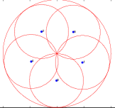
(a) Global Solution: $o=.4122147478$

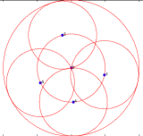
(b) Local Solution: $o=.5$

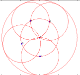
(c) Local Solution: $o=.5$

Fig. 1: Solutions obtained by Algorithm 1 for packing circles of radius $.5$ into a circle of radius $1$, showing final overlap measures for each.

Example 3.1 (Five Circles).

Consider the problem of packing five circles of radius .5 into an enclosing circle of radius 1. Results obtained with Algorithm 1, with objective $H(\xi)=\|\xi\|_{\infty}$, from random starting points reveal an apparent global solution (Figure 1(a)) and a family of local solutions (Figures 1(b) and 1(c)). The local solutions are characterized by one of the packed circles having its center at the center of the enclosing circle; this circle thus has an overlap of .5 with all four of the outer circles. The outer circles in this local solution need only be arranged so that their maximum pairwise overlap is no greater than .5. Algorithm 1 required only a few iterations for each of these examples.

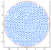
Fig. 2: Circle packing in a circular enclosure. A nearly hexagonal arrangement is seen in the interior.

As noted in Section 1 optimal sphere packings (configurations with no overlap) have been obtained in two and three dimensions, for spaces of infinite extent. Our algorithm can only solve problems with finite enclosing shapes, but we can use large enclosures to investigate how similar the local solutions attained by our algorithm are to the known optimal packings in $\makebox{\sf I R }^{2}$ (hexagonal lattice with density $\pi/\sqrt{12}$) and $\makebox{\sf I R }^{3}$ (FCC lattice with density $\pi/\sqrt{18}$).

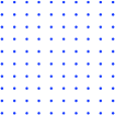
(a) $o=.1192514295$

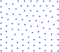
(b) $o=.1188906843$

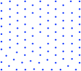
(c) $o=.1181440939$

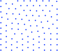
(d) $o=.1179656050$

Fig. 3: Local minima obtained by Algorithm 1 for packing circles into a square, showing final overlap measures for each.

Example 3.2 (Uniform Circles in $\makebox{\sf I R }^{2}$).

We ran Algorithm 1 with $N=150$ circles, each of area $\pi$, and a circular container of size $150\sqrt{12}$. This results in a total circle area-to-container area ratio which is equal to the optimal packing density. The resulting circle configuration is shown in Figure 2. The hexagonal arrangement of the circles is clearly visible in the interior of the container.

We also ran tests in which 100 circles are packed into a square container. (Rectangular feasible sets $\Omega_{i}$ are easily incorporated into the formulation by defining bound constraints on the centers $c_{i}$.) We generate starting points by arranging the centers in a $10\times 10$ square lattice. We may then add a random perturbation to each center. Results are shown in Figure 3. (For clarity, we show only the centers in this figure, omitting the circles.) When no perturbations are added to the starting configuration, the algorithm does not move from the initial square configuration shown in Figure 3(a). When random initial perturbations are applied (large enough that the original square grid structure is not recognizable in the initial point), many different local minima are obtained. Three of these are shown in Figures 3(b), 3(c), and 3(d). Note that all of these have a maximum overlap less than the square configuration, and that hexagonal structure is recognizable in large parts of the domain, with square structure and disorder in intermediate regions.

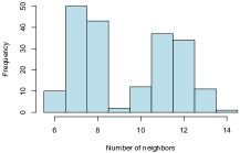
(a) Distribution of neighbor counts.

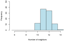
(b) Distribution of neighbor counts, after spheres at the periphery have been removed.

Fig. 4: Neighbor counts for packing of 100 three-dimensional spheres in in a spherical container.

Example 3.3 (Uniform spheres in $\makebox{\sf I R }^{3}$).

We performed a similar test to Example 3.2 in three dimensions. We checked to see whether Algorithm 1 converges to a solution like the FCC lattice in a finite minimum-overlap arrangement with 200 spheres enclosed in a larger sphere. We chose the small spheres to have volume $\pi$ and the containing sphere to have volume $200\sqrt{18}$, giving a density of $\pi/\sqrt{18}$, identical to the FCC lattice, which is optimal in infinite space. At the solution obtained by Algorithm 1, we counted the number of spheres that touch or intersect each sphere. This statistic provides an indication of the type of packing attained, since the FCC lattice has 12 neighbors per sphere, while the BCC lattice has only 8 neighbors per sphere. The histogram for the number of neighboring spheres is shown in Figure 4(a). A more instructive diagram is obtained by removing from consideration those spheres that touch the enclosing sphere. After doing so, we obtain the histogram in Figure 4(b). This figure suggests strongly that the calculated solution is close to the FCC lattice over most of the interior region of the domain.

Finally, we report on solutions obtained by Algorithm 1 on packings of discs in a circle, for which the optimal packing is known in only a few cases. In particular, we analyze packings with equally sized discs, where the number of discs is given by a hexagonal number, that is,

$$h(k)=3k(k+1)+1,\qquad k\geq 1.$$ (17)

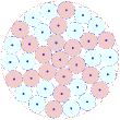
(a) $37$ discs

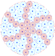
(b) $61$ discs

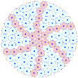
(c) $91$ discs

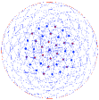
(d) $37$ discs, larger radii

Fig. 5: Optimal configurations found using Algorithm 1 for hexagonal numbers of unit discs in an enclosing circle.

Example 3.4.

Lubachevsky and Graham [10] introduce curved hexagonal packings, a new family of packings for configurations with a hexagonal number of discs. This family contains the best packings found so far for $h(k)$ defined by (17), for $k\leq 5$. We ran Algorithm 1 with the optimal densities found in [10] for $k=3,4,5$. The best local optima we found are shown in Figure 5; they are identical to the configurations found in [10]. (We highlight some of the circles to emphasize the “curved” feature of the packing, which distinguishes it from a standard hexagonal arrangement, which has slightly lower density when restricted to a finite circle.)

When we ran Algorithm 1 on the problem of 37 uniform discs in a larger disc, where the radii were too large to allow packing without overlap, the algorithm with $H(\xi)=\|\xi\|_{\infty}$ produced the same arrangement of centers as in Figure 5(a) (see Figure 5(d)) when initialized at a sufficiently close initial point. It is a well known property of minimization of the norm $\|\cdot\|_{\infty}$ that many elements of the argument vector tend to achieve the maximum value. In our application, this means that the maximal overlap is attained by many pairs of circles. We can obtain non-overlapping configurations by simply reducing the radii of all discs uniformly, by an amount equal to half the maximal overlap. This will yield a solution in which each pair of circles that formerly overlapped maximally now just touches.

4 Ellipsoid Packing

Here we discuss a bilevel optimization procedure for packing ellipsoids into an ellipsoidal container in a way that minimizes the maximum overlap of any pair of ellipsoids. It is not as obvious how to measure the overlap between two ellipsoids as between two spheres, since it depends on the orientation of the ellipsoids as well as the location of their centers. We measure the overlap by the sum of principal semi-axes of the largest ellipsoid that can be inscribed in the intersection of the two ellipsoids. This overlap measure can be calculated by solving a small semidefinite optimization problem, constructed according to the S-procedure (see Subsection 4.1). These are the lower-level problems in our bilevel optimization formulation. The upper-level problem is to position and orient the ellipsoids so as to minimize the maximum overlap (see Subsection 4.2), while keeping all ellipsoids inside the enclosing shape. We refer to this problem as “min-max-overlap.” Dual information from the lower-level problems provides a measure of sensitivity of the overlaps to the ellipsoid parameters, allowing us to develop a successive approximation approach, with trust regions, whose accumulation points are stationary for the min-max-overlap problem. Technical results regarding the trust-region approach and the proof of convergence are given in Subsection 4.3.

4.1 Measuring Overlap

Boyd and Vandenberghe [3, Section 8.4.2] consider the problem of finding the ellipsoid of largest volume inscribed in an intersection of ellipsoids. The volume of an ellipsoid $\mathcal{E}=\{c+Su\mid\lVert u\rVert_{2}\leq 1\}$ is proportional to $\det(S)$. Although this problem is convex, it is not a semidefinite program (SDP), because the objective is nonlinear. We thus consider an alternative in which $\mbox{\rm trace}(S)$ is used as the objective. The trace is the sum of lengths of the semi-axes of the ellipsoid, which is a good proxy for the volume in problems of the type we consider. Trace maximization admits an SDP formulation of the lower-level problems, which facilitates theoretical development and analysis of our min-max-overlap problem.

Recalling from (3) that we define the ellipsoid $\mathcal{E}_{i}$ by

$$\mathcal{E}_{i}:=\{c_{i}+S_{i}u\mid\|u\|_{2}\leq 1\},$$ (18)

we introduce the notation $\Sigma_{i}=S_{i}^{2}$. Parametrizing the inscribed ellipsoid similarly by $\mathcal{E}_{ij}:=\{c_{ij}+S_{ij}u\mid\|u\|_{2}\leq 1\}$, and using (5) to formulate the fact that the inscribed ellipsoid is contained in both $\mathcal{E}_{i}$ and $\mathcal{E}_{j}$, we formulate the problem of measuring overlap as follows:

$$\hat{O}(c_{i},c_{j},\Sigma_{i},\Sigma_{j}):=\max_{S_{ij}\succeq 0,c_{ij},\lambda_{ij1},\lambda_{ij2}}\; \mbox{\rm trace}(S_{ij})$$

subject to $$\begin{pmatrix}-\lambda_{ij1}I&0&S_{ij}\\ 0&\lambda_{ij1}-1&(c_{ij}-c_{i})^{T}\\ S_{ij}&c_{ij}-c_{i}&-\Sigma_{i}\end{pmatrix}\preceq 0,$$ (19a)

$$\begin{pmatrix}-\lambda_{ij2}I&0&S_{ij}\\ 0&\lambda_{ij2}-1&(c_{ij}-c_{j})^{T}\\ S_{ij}&c_{ij}-c_{j}&-\Sigma_{j}\end{pmatrix}\preceq 0.$$ (19b)

The Lagrangian can be written as

$${\cal L}(c,S_{ij},\lambda_{ij1},\lambda_{ij2},T_{ij},M_{ij1},M_{ij2}):= \langle I,S_{ij}\rangle+\langle T_{ij},S_{ij}\rangle$$

$$-\langle M_{ij1},\begin{pmatrix}-\lambda_{ij1}I&0&S_{ij}\\ 0&\lambda_{ij1}-1&(c_{ij}-c_{i})^{T}\\ S_{ij}&c_{ij}-c_{i}&-\Sigma_{i}\end{pmatrix}\rangle$$

$$-\langle M_{ij2},\begin{pmatrix}-\lambda_{ij2}I&0&S_{ij}\\ 0&\lambda_{ij2}-1&(c_{ij}-c_{j})^{T}\\ S_{ij}&c_{ij}-c_{j}&-\Sigma_{j}\end{pmatrix}\rangle,$$

with the dual problem being derived from

$$\min_{M_{ij1}\succeq 0,M_{ij2}\succeq 0,T_{ij}\succeq 0}\,\left\{\max_{S_{ij}\succeq 0,c_{ij},\lambda_{ij1},\lambda_{ij2}}\,{\cal L}(c_{ij},S_{ij},\lambda_{ij1},\lambda_{ij2},T_{ij},M_{ij1},M_{ij2})\right\}.$$

Introducing the following notation for $M_{ij1}$ and $M_{ij2}$:

$$M_{ij1}:=\begin{pmatrix}R_{ij1}&r_{ij1}&P_{ij1}\\ r_{ij1}^{T}&p_{ij1}&q_{ij1}^{T}\\ P_{ij1}&q_{ij1}&Q_{ij1}\end{pmatrix},\qquad M_{ij2}:=\begin{pmatrix}R_{ij2}&r_{ij2}&P_{ij2}\\ r_{ij2}^{T}&p_{ij2}&q_{ij2}^{T}\\ P_{ij2}&q_{ij2}&Q_{ij2}\end{pmatrix},$$ (20)

we can write the dual explicitly as follows:

$$\hat{O}(c_{i},c_{j},\Sigma_{i},\Sigma_{j}):=\min_{M_{ij1}\succeq 0,M_{ij2}\succeq 0,T_{ij}\succeq 0}\qquad p_{ij1}+p_{ij2}+2q_{ij1}^{T}c_{i}+2q_{ij2}^{T}c_{j}$$

$$\qquad+\langle Q_{ij1},\Sigma_{i}\rangle+\langle Q_{ij2},\Sigma_{j}\rangle$$

subject to $$0=I+T_{ij}-2P_{ij1}-2P_{ij2}$$ (21)

$$0=\mbox{\rm trace}(R_{ij1})-p_{ij1}$$

$$0=\mbox{\rm trace}(R_{ij2})-p_{ij2}$$

$$0=q_{ij1}+q_{ij2}.$$

(We have assumed without loss of generality that $P_{ij1}$ and $P_{ij2}$ are in $S\makebox{\sf I R }^{n\times n}$; this follows from $S_{ij}\in S\makebox{\sf I R }^{n\times n}$.)

When the ellipsoids ${\cal E}_{i}$ and ${\cal E}_{j}$ overlap, strong duality holds for this primal-dual pair of semidefinite programs since, as we now verify, both problems have a strictly feasible point. For (19) we know that there exists an ellipsoid with positive volume that is strictly inscribed in the intersection. By setting $c_{ij}$ and $S_{ij}$ to be the parameters of this ellipsoid (with $S_{ij}\succ 0$), the S-procedure for strict inequalities can be applied to show that (strict) definiteness holds in (19a) and (19b). This fact establishes strict feasibility of (19). For the dual (4.1), we can set $T_{ij}=I$ and define

$$M_{ij1}=M_{ij2}=\begin{pmatrix}I&0&\frac{1}{2}I\\ 0&n&0\\ \frac{1}{2}I&0&I\end{pmatrix}.$$

It is easy to verify that these choices satisfy the constraints in (4.1), along with the (strict) interiority conditions $M_{ij1}\succ 0$, $M_{ij2}\succ 0$, $T_{ij}\succ 0$. This observation of strong duality justifies our use of the notation $\hat{O}(c_{i},c_{j},\Sigma_{i},\Sigma_{j})$ to denote the optimal objectives of both primal and dual.

4.2 Choosing Ellipse Positions and Orientations

The main variables in the min-max-overlap problem are the parameters defining the ellipses $\mathcal{E}_{i}$ for $i=1,2,\dotsc,N$: the centers $c_{i}$ and the orientations defined by $S_{i}$ (and thus $\Sigma_{i}=S_{i}^{2}$). For $n=3$ (which we assume in this section and subsequently), we would like to fix the lengths of the axes of each ellipsoid at the values $r_{i1}$, $r_{i2}$, and $r_{i3}$ (assuming that $r_{i1}\geq r_{i2}\geq r_{i3}$). This is equivalent to fixing the eigenvalues of $\Sigma_{i}$ at $r_{i1}^{2}$, $r_{i2}^{2}$, and $r_{i3}^{2}$, or to fixing the eigenvalues of $S_{i}$ to $r_{i1}$, $r_{i2}$, and $r_{i3}$.

Using the notation $\hat{O}$ defined in (19) and (4.1), we can formulate the min-max-overlap problem as the following bilevel optimization problem:

$$\min_{\xi,(c_{i},S_{i},\Sigma_{i}),i=1,2,\dotsc,N}\; \xi$$ (22a)

subject to $$\xi\geq\hat{O}(c_{i},c_{j},\Sigma_{i},\Sigma_{j}), 1\leq i<j\leq N,$$ (22b)

$$\mathcal{E}_{i}\subset\mathcal{E}, i=1,2,\dots,N,$$ (22c)

$$\Sigma_{i}=S_{i}^{2},$$ (22d)

$$\mbox{semi-axes of }\mathcal{E}_{i}\mbox{ have lengths }r_{i1},r_{i2},r_{i3}, i=1,2,\dots,N.$$ (22e)

This problem is nonconvex for three reasons. First, each pairwise overlap objective $\hat{O}(c_{i},c_{j},\Sigma_{i},\Sigma_{j})$ is a nonconvex function of its arguments. This issue is intrinsic; as in the sphere-packing problem, we expect there to be many local solutions and we can only expect our algorithm to find one of them. As we see below (in (27) and Algorithm 2), our algorithm iteratively solves subproblems in which each $\hat{O}$ is replaced by a linearized approximation that makes use of the optimal dual variables $M_{ij1}$ and $M_{ij2}$ from the formulation (4.1). These subproblems will be convex if we can overcome the other two sources of nonconvexity in the formulation (22), which we address now.

The second nonconvexity issue is in the constraint (22e) on the eigenvalues of $S_{i}$, $i=1,2,\dotsc,N$. We consider instead the following convex relaxation:

$$S_{i}-r_{i1}I\preceq 0,\quad S_{i}-r_{i3}I\succeq 0,\quad\mbox{\rm trace}(S_{i})=r_{i1}+r_{i2}+r_{i3}.$$ (23)

Note that this is indeed a relaxation: If $\mathcal{E}_{i}$ has the desired dimensions, then the eigenvalues of $S_{i}$ are $r_{i1}$, $r_{i2}$, and $r_{i3}$, and the conditions (23) are satisfied. Because the overall goal is to minimize maximal overlap, and because minimum-volume ellipsoids are those that are most eccentric, the relaxation (23) is usually “tight” with respect to (22) in many interesting cases. Intermediate iterates are often observed to have ellipsoids less eccentric than desired.

The third source of nonconvexity — the constraint (22d) — is relatively easy to deal with. We replace it with the following pair of restrictions:

$$\left[\begin{matrix}\Sigma_{i}&S_{i}\\ S_{i}&I\end{matrix}\right]\succeq 0,\qquad S_{i}\succeq 0,\qquad i=1,2,\dotsc,N.$$ (24)

The first of these conditions ensures only that $\Sigma_{i}\succeq S_{i}^{2}$. However, the overlap $\hat{O}(c_{i},c_{j},\Sigma_{i},\Sigma_{j})$ will grow if $\Sigma_{i}$ is replaced by any matrix $\tilde{\Sigma}_{i}\succeq\Sigma_{i}$. Hence, because of the min-max-overlap objective in (22), the matrices $\Sigma_{i}$ will be set to the “smallest possible values” that satisfy the conditions (24), that is, $\Sigma_{i}=S_{i}^{2}$.

Finally, defining the containing ellipse to be $\mathcal{E}:=\{x\mid(x-c)^{T}\Sigma^{-1}(x-c)\leq 1\}$, we can use (5) to formulate the condition (22c) as follows:

$$\left[\begin{matrix}-\lambda_{i}I&0&S_{i}\\ 0&\lambda_{i}-1&(c_{i}-c)^{T}\\ S_{i}&c_{i}-c&-\Sigma\end{matrix}\right]\preceq 0,$$ (25)

Given all these considerations, we define the relaxed version of (22) to be addressed in this section as follows:

$$\min_{\xi,(\lambda_{i},c_{i},S_{i}\Sigma_{i}),i=1,2,\dotsc,N}\;\;\; \xi$$ (26a)

subject to $$\xi\geq\hat{O}(c_{i},c_{j},\Sigma_{i},\Sigma_{j}), 1\leq i<j\leq N,$$ (26b)

$$\left[\begin{matrix}-\lambda_{i}I&0&S_{i}\\ 0&\lambda_{i}-1&(c_{i}-c)^{T}\\ S_{i}&c_{i}-c&-\Sigma\end{matrix}\right]\preceq 0, i=1,2,\dotsc,N,$$ (26c)

$$\left[\begin{matrix}\Sigma_{i}&S_{i}\\ S_{i}&I\end{matrix}\right]\succeq 0, i=1,2,\dotsc,N,$$ (26d)

$$S_{i}-r_{i1}I\preceq 0,\quad S_{i}-r_{i3}I\succeq 0, i=1,2,\dots,N,$$ (26e)

$$\mbox{\rm trace}(S_{i})=r_{i1}+r_{i2}+r_{i3}, i=1,2,\dots,N.$$ (26f)

Note that when the ellipse $\mathcal{E}_{i}$ is actually a circle, that is, $r_{i1}=r_{i2}=r_{i3}$, we can fix $S_{i}=r_{i1}I$ and $\Sigma_{i}=r_{i1}^{2}I$ in (27), and eliminate these variables from that problem. Hence, we can assume without loss of generality that $r_{i1}>r_{i3}$.

In the remainder of this subsection, we describe our algorithm for solving the bilevel optimization problem (26), and prove convergence properties. Our development and analysis takes place in a general setting that encompasses (26) but uses simpler notation. A key step in the algorithm is the solution of a subproblem for (26) in which the objective is linearized using the optimal values from the dual overlap formulation (4.1). The other constraints in (26) remain the same, and a trust region is added to restrict the amount by which the ellipsoid parameters can change. This subproblem can be stated as follows:

$$\min_{\xi,(\lambda_{i},c_{i},S_{i},\Sigma_{i}),i=1,2,\dotsc,N}\;\;\; \xi$$ (27a)

subject to $$\xi\geq p_{ij1}+p_{ij2}+2q_{ij1}^{T}c_{i}+2q_{ij2}^{T}c_{j}$$

$$\qquad\,\,+\langle Q_{ij1},\Sigma_{i}\rangle+\langle Q_{ij2},\Sigma_{j}\rangle, \mbox{for }(i,j)\in{\cal I},$$ (27b)

$$\left[\begin{matrix}-\lambda_{i}I&0&S_{i}\\ 0&\lambda_{i}-1&(c_{i}-c)^{T}\\ S_{i}&c_{i}-c&-\Sigma\end{matrix}\right]\preceq 0, i=1,2,\dotsc,N,$$ (27c)

$$\left[\begin{matrix}\Sigma_{i}&S_{i}\\ S_{i}&I\end{matrix}\right]\succeq 0, i=1,2,\dotsc,N,$$ (27d)

$$S_{i}-r_{i1}I\preceq 0,\quad S_{i}-r_{i3}I\succeq 0, i=1,2,\dots,N,$$ (27e)

$$\mbox{\rm trace}(S_{i})=r_{i1}+r_{i2}+r_{i3}, i=1,2,\dots,N,$$ (27f)

$$\lVert c_{i}-c_{i}^{-}\rVert_{2}^{2}\leq\Delta_{c}^{2}, i=1,2,\dots,N,$$ (27g)

$$\lVert S_{i}-S_{i}^{-}\rVert\leq\Delta_{S}, i=1,2,\dots,N,$$ (27h)

$$|\lambda_{i}-\lambda_{i}^{-}|\leq\Delta_{\lambda}, i=1,2,\dots,N.$$ (27i)

Here, $(\lambda_{i}^{-},c_{i}^{-},S_{i}^{-},\Sigma_{i}^{-})$ are the values of the variables at the current iteration, and $\Delta_{c}$, $\Delta_{S}$, and $\Delta_{\lambda}$ are trust-region radii. The quantities $p_{ij1}$, $p_{ij2}$, $q_{ij1}$, $q_{ij2}$, $Q_{ij1}$, and $Q_{ij2}$ are extracted from the dual solutions $M_{ij1}$ and $M_{ij2}$ of (4.1) according to the structure (20). The set ${\cal I}$ represents a subset of all possible pairs $(i,j)$ for $1\leq i<j\leq N$, representing some selection of ellipses which currently have a (strict) overlap. Further details on the choice of ${\cal I}$ are given in Subsection 4.4.

We claim first that, if it is possible to fit each ellipsoid $\mathcal{E}_{i}$ strictly inside the enclosing ellipsoid $\mathcal{E}$, the subproblem (27) satisfies a Slater condition. That is, there exists a point that satisfies the linear equality constraints and strictly satisfies the inequality constraints in this problem. To justify this claim, we first show that it is possible to find a point $(\bar{\lambda_{i}},\bar{c}_{i},\bar{S}_{i},\bar{\Sigma}_{i})$ that satisfies the following conditions:

$$\left[\begin{matrix}-\bar{\lambda}_{i}I&0&\bar{S}_{i}\\ 0&\bar{\lambda}_{i}-1&(\bar{c}_{i}-c)^{T}\\ \bar{S}_{i}&\bar{c}_{i}-c&-\Sigma\end{matrix}\right] \prec 0, i=1,2,\dotsc,N,$$ (28a)

$$\left[\begin{matrix}\bar{\Sigma}_{i}&\bar{S}_{i}\\ \bar{S}_{i}&I\end{matrix}\right] \succ 0, i=1,2,\dotsc,N,$$ (28b)

$$\bar{S}_{i}-r_{i1}I\prec 0,\quad\bar{S}_{i}-r_{i3}I \succ 0, i=1,2,\dots,N,$$ (28c)

$$\mbox{\rm trace}(S_{i})=r_{i1}+r_{i2}+r_{i3}, i=1,2,\dots,N.$$ (28d)

First, choosing $\bar{c}_{i}=c$ in (28a), and orienting ellipsoid $\mathcal{E}_{i}$ appropriately, we can find $\bar{\lambda}_{i}>0$ such that (28a) is satisfied. This remains true if we perturb $\bar{S}_{i}$ slightly so that its spectrum lies in the open interval $(r_{i3},r_{i1})$ while still satisfying the trace condition (28d). This perturbed $\bar{S}_{i}$ thus satisfies the conditions (28c). Second, we can simply define $\bar{\Sigma}_{i}=\sigma_{i}I$ for large enough $\sigma_{i}>0$ to ensure that (28b) is satisfied strictly.

Next, note that from the current iteration, we have a point $(\lambda_{i}^{-},c_{i}^{-},S_{i}^{-},\Sigma_{i}^{-})$ that satisfies the constraints of (26), that is,

$$\left[\begin{matrix}-\lambda_{i}^{-}I&0&S_{i}^{-}\\ 0&\lambda_{i}^{-}-1&(c_{i}^{-}-c)^{T}\\ S_{i}^{-}&c_{i}^{-}-c&-\Sigma\end{matrix}\right] \preceq 0, i=1,2,\dotsc,N,$$ (29a)

$$\left[\begin{matrix}\Sigma_{i}^{-}&S_{i}^{-}\\ S_{i}^{-}&I\end{matrix}\right] \succeq 0, i=1,2,\dotsc,N,$$ (29b)

$$S_{i}^{-}-r_{i1}I\preceq 0,\quad S_{i}^{-}-r_{i3}I \succeq 0, i=1,2,\dots,N,$$ (29c)

$$\mbox{\rm trace}(S_{i}^{-})=r_{i1}+r_{i2}+r_{i3}, i=1,2,\dots,N.$$ (29d)

It is now easy to check that for sufficiently small $\epsilon>0$, the point

$$(\lambda_{i}(\epsilon),c_{i}(\epsilon),S_{i}(\epsilon),\Sigma_{i}(\epsilon)):=(1-\epsilon)(\lambda_{i}^{-},c_{i}^{-},S_{i}^{-},\Sigma_{i}^{-})+\epsilon(\bar{\lambda_{i}},\bar{c}_{i},\bar{S}_{i},\bar{\Sigma}_{i})$$

satisfies the inequalities (27c), (27d), and (27e) strictly, satisfies the linear constraint (27f), and satisfies the trust-region constraints (27g), (27h), and (27i) strictly. Since we can choose $\xi$ arbitrarily large to strictly satisfy (27b), we conclude that there exists a Slater point for (27).

4.3 Technical Results

We prove here some technical results that provide the basis for convergence of the trust-region strategy. To simplify the notation, we note that each dual overlap problem (4.1) has the general form

$$P(l,C):\qquad t^{*}_{l}(C):= \min_{M_{l}}\;\langle C,M_{l}\rangle$$ (30a)

$$\,\,\mbox{s.t.}\,\,\langle A_{l,i},M_{l}\rangle=b_{l,i},\;\;i=1,2,\dotsc,p_{l},\;\;M_{l}\succeq 0.$$ (30b)

Here $C$ captures the parameters that describe all the ellipses, and $M_{l}$ is the dual variable for the overlap problem. We assume that $C$ lies in a set $\Omega$ of the following form:

$$\Omega:=\bar{\Omega}\cap\{C\,:\,\langle B_{k},C\rangle=b_{k},\ k=1,2,\dotsc,p\},$$ (31)

where $\bar{\Omega}$ is closed, convex, bounded, with nonempty interior. We now verify formally that the ellipse parameters satisfying the constraints in (26) can be expressed in the form (31). We define $C$ to be a block-diagonal matrix with $N$ blocks of the form:

$$\left[\begin{matrix}\Sigma_{i}&c_{i}\\ c_{i}^{T}&1\end{matrix}\right],\quad i=1,2,\dotsc,N,$$ (32)

and define $\bar{\Omega}$ to be the set of all symmetric matrices of this form for which there exist $\lambda_{i}$ and $S_{i}$ such that each tuple $(\lambda_{i},c_{i},S_{i},\Sigma_{i})$ satisfies the conditions (26c), (26d), and (26e). Boundedness of $c_{i}$ is obvious from the containment condition $\mathcal{E}_{i}\subset\mathcal{E}$; boundedness of $S_{i}$ follows from (26e); while (26c) implies that $\lambda_{i}\in[0,1]$. Boundedness of $\Sigma_{i}$ is not guaranteed by the constraints in (26). We could, however, add the constraint $\Sigma_{i}\preceq r_{i1}^{2}I$ without changing the solution of the problem, thus completing the verification of boundedness of $\bar{\Omega}$. (For simplicity, however, we do not put this explicit bound on $\Sigma_{i}$ in our discussion below.) Closedness and convexity are immediate consequence of the form of the constraints (26c), (26d), and (26e). To verify nonemptiness of the interior of $\bar{\Omega}$, recall the discussion following (26), where we noted that variable $S_{i}$ can be eliminated from the formulation if ellipsoid $\mathcal{E}_{i}$ is in fact a circle. Thus, we can assume without loss of generality that $r_{i1}>r_{i3}$ for all $i$, and hence, from the discussion surrounding (28), we conclude that the set of tuples $(\lambda_{i},c_{i},S_{i},\Sigma_{i})$ allowed by constraints (26c), (26d), and (26e) has nonempty interior. The structural features of $C$ (the diagonal element $1$ in (32) and the off-diagonal zeros) can in principle be enforced by affine constraints of the form given in (31). The constraints (26f) can also be enforced in this way.

Following the notation of (28), we denote by $\bar{C}$ the point that satisfies

$$\bar{C}\in\mbox{\rm int}\,\bar{\Omega}\quad\mbox{and}\quad\langle B_{k},\bar{C}\rangle=b_{k},\ k=1,2,\dotsc,p.$$ (33)

We denote by $M_{l}(C)$ an optimal value of $M_{l}$ in (30) (not necessarily unique).

The primal form (19) of the overlap problem (30) has the form

$$\max_{\zeta_{l}=(\zeta_{l,1},\zeta_{l,2},\dotsc,\zeta_{l,p_{l}})}\,b_{l}^{T}\zeta_{l}\quad\mbox{s.t.}\quad C-\sum_{i=1}^{p_{l}}\zeta_{l,i}A_{l,i}\succeq 0.$$ (34)

As discussed in Subsection 4.1, both (30) and (34) have strictly feasible points when there is positive overlap between two ellipsoids. Therefore, strong duality holds, so the following optimality conditions relating the solutions of (30) and (34) are satisfied:

$$0\preceq M_{l} \perp C-\sum_{i=1}^{p_{l}}\zeta_{l,i}A_{l,i}\succeq 0$$ (35a)

$$\langle A_{l,i},M_{l}\rangle =b_{l,i},\;\;i=1,2,\dotsc,p_{l}.$$ (35b)

By convention, we set $t^{*}_{l}(C)=-\infty$ if (30) is infeasible, that is, if there is no overlap between the two ellipses corresponding to index $l$. By the nature of the problem, we know that $t^{*}_{l}(C)>0$ if these two ellipses have positive overlap. It is easy to see that $t^{*}_{l}(C)$ is a concave, extended-valued function of $C\in\Omega$, and as a consequence that $t^{*}_{l}(C)$ is continuous on the relative interior of its domain. Further useful facts about $t^{*}_{l}(C)$ are given in Lemma 12. These include Lipschitz continuity in a neighborhood of a point $C$ at which (34) has a strictly interior point (which, as noted in Subsection 4.1, occurs when the two ellipsoids have positive overlap), and the fact that any solution $M_{l}(C)$ of (30) belongs to the Clarke subdifferential of $t^{*}_{l}(C)$.

Using the notation of (30) and (34) to capture the min-max-overlap problem (22), we can state this problem as follows:

$$\min_{C\in\Omega}\;\;t^{*}(C):=\max_{l=1,2,\dotsc,m}\,t_{l}^{*}(C).$$ (36)

Here each element in $\{1,2,\dotsc,m\}$ represents the overlap problem for a given pair of ellipsoids. Note that $t^{*}(C)=-\infty$ if no pair of ellipsoids overlaps or touches.

We now define the subproblems to be solved at each iteration of the algorithm, which depend on just a subset ${\cal F}\subset\{1,2,\dotsc,m\}$ of the individual overlap problems. The key quantity is defined as follows

$$t^{*}_{{\cal F}}(C):=\max_{l\in{\cal F}}\,t^{*}_{l}(C),$$ (37)

where ${\cal F}$ is a subset of the strictly overlapping ellipsoid pairs, that is,

$${\cal F}\subset\{l=1,2,\dotsc,m\,:\,t^{*}_{l}(C)>0\}.$$

(We will be more specific about the definition of ${\cal F}$ later.) In the algorithm, the solutions $M_{l}(C)$ of (30) for $l\in{\cal F}$ are used to construct a linearized subproblem whose solution is a step $\Delta C$ in the parameter $C$, assuming that the current $C$ is feasible. The subproblem is as follows:

$$L({\cal F},C,M_{{\cal F}}(C),\rho):\qquad r({\cal F},C,M_{{\cal F}}(C),\rho):=\min_{r,\Delta C}\,r$$ (38a)

s.t. $$r\geq t^{*}_{l}(C)+\langle\Delta C,M_{l}(C)\rangle,\;\;l\in{\cal F},$$ (38b)

$$C+\Delta C\in\Omega,\;\;\;\|\Delta C\|\leq\rho.$$ (38c)

Here $\rho>0$ is a trust-region radius, and $M_{{\cal F}}(C)$ denotes the set of matrices $\{M_{l}(C)\,:\,l\in{\cal F}\}$. The problem (38) is convex, and its feasible set is bounded, so it has an optimal value which we denote by $\Delta C(\rho)$. Further, the KKT conditions are satisfied at this point. This claim follows from the fact that, given the point $\bar{C}$ satisfying (33), and defining $\Delta C=\epsilon(\bar{C}-C)$ for some small positive $\epsilon>0$, we have that

$$C+\Delta C=(1-\epsilon)C+\epsilon\bar{C}\in\mbox{\rm int}\,\Omega,$$

while the trust-region condition is strictly satisfied ($\|\epsilon(\bar{C}-C)\|<\rho$), and the remaining constraints in (38) are affine. Hence, the conditions of [13, Theorem 28.2] are satisfied, and we can apply [13, Corollary 28.3.1] to deduce that there exist $\mu_{l}$, $l\in{\cal F}$ and $\tau\geq 0$ such that

$$1-\sum_{l\in{\cal F}}\mu_{l}=0,$$ (39a)

$$0\leq\mu_{l}\perp r({\cal F},C,M_{{\cal F}}(C),\rho)-t^{*}_{l}(C)-\langle\Delta C,M_{l}(C)\rangle\geq 0,\;\;l\in{\cal F},$$ (39b)

$$-\sum_{l\in{\cal F}}\mu_{l}M_{l}(C)-\tau u\in N_{\Omega}(C+\Delta C)\;\;\mbox{for some $u\in\partial\|\Delta C\|$,}$$ (39c)

$$C+\Delta C\in\Omega,$$ (39d)

$$0\leq\tau\perp\rho-\|\Delta C\|\geq 0.$$ (39e)

Here $N_{\Omega}(C)$ denotes the normal cone to the closed convex set $\Omega$ at the point $C$ (see (1)) and $\partial$ denotes a subdifferential. (As noted in Section 1, since $\|\cdot\|$ is convex and Lipschitz continuous, the Clarke subdifferential coincides with the subdifferential from convex analysis.) Note that the set $\{\tau v\,:\,\tau\geq 0,\;v\in\partial\|\Delta C\|\}$ is a closed convex cone and that it is an outer semicontinuous set-valued function of $\Delta C$.

It is sometimes convenient to rewrite $L({\cal F},C,M_{{\cal F}}(C),\rho)$ by defining the function

$$G_{{\cal F}}(\Delta C;C,M_{{\cal F}}(C)):=\max_{l\in{\cal F}}\,\langle C+\Delta C,M_{l}(C)\rangle,$$ (40)

and writing

$$L({\cal F},C,M_{{\cal F}}(C),\rho):\;\;\min_{\Delta C}\,G_{{\cal F}}(\Delta C;C,M_{{\cal F}}(C))\;\;\mbox{s.t.}\;\;C+\Delta C\in\Omega,\;\;\|\Delta C\|\leq\rho.$$ (41)

Note that $G_{{\cal F}}(\cdot;C,M_{{\cal F}}(C))$ is convex, in fact piecewise linear.

Next, we define the reference problem $P({\cal F})$ that minimizes $t^{*}_{{\cal F}}(C)$ defined in (37) over $C\in\Omega$:

$$P({\cal F}):\qquad t^{*}_{{\cal F}}:=\min_{C\in\Omega}\,t^{*}_{{\cal F}}(C)=\min_{C\in\Omega}\,\max_{l\in{\cal F}}\,t^{*}_{l}(C).$$ (42)

Nonsmooth analysis provides the following result that characterizes solutions of (42).

Lemma 4.

Suppose that for a given set ${\cal F}\subset\{1,2,\dotsc,m\}$, $\bar{C}$ is a local solution of (42) at which (34) has a strictly interior point, for all $l\in{\cal F}$. Define $\bar{{\cal F}}(\bar{C})$ to be the set of indices achieving the maximum in (42), that is, $\bar{{\cal F}}(\bar{C})=\{l\in{\cal F}\,:\,t^{*}_{l}(\bar{C})=t^{*}_{{\cal F}}\}$. Then there exist $\bar{M}_{l}\in\partial t^{*}_{l}(\bar{C})$ and scalars $\mu_{l}$, for all $l\in\bar{{\cal F}}(\bar{C})$, such that

$$-\sum_{l\in\bar{{\cal F}}(\bar{C})}\mu_{l}\bar{M}_{l}\in N_{\Omega}(\bar{C}),\quad\sum_{l\in\bar{{\cal F}}(\bar{C})}\mu_{l}=1,\quad\mu_{l}\geq 0,\;l\in\bar{{\cal F}}(\bar{C}),\quad\bar{C}\in\Omega.$$ (43)

Proof.

We appeal to results about the Clarke subdifferential applied to max-functions and sums of functions. First, note that the strict interiority assumption means that we can apply Lemma 12 (iv) to deduce that each $t^{*}_{l}$ is Lipschitz continuous in a neighborhood of $\bar{C}$. Hence, applying [2, Theorem 6.1.5], we have that

$$\partial\,t^{*}_{{\cal F}}(C)\subset\mbox{conv}\{\partial t^{*}_{l}(\bar{C})\,:\,l\in\bar{{\cal F}}(\bar{C})\},$$ (44)

where $\mbox{conv}(\cdot)$ denotes the convex hull. The Corollary in [4, p. 52] can be used to show that when $\bar{C}$ is a solution of (42), we have

$$0\in\partial\,t^{*}_{{\cal F}}(\bar{C})+N_{\Omega}(\bar{C}).$$

The result follows by combining this expression with (44). ∎

By introducing multipliers for the indices $l\in{\cal F}\setminus\bar{{\cal F}}(\bar{C})$, we can restate the conditions (43) as follows:

$$0\leq\mu_{l}\perp t^{*}_{{\cal F}}-t^{*}_{l}(\bar{C})\geq 0,\qquad\mbox{for all $l\in{\cal F}$,}$$ (45a)

$$\sum_{l\in{\cal F}}\mu_{l}=1,$$ (45b)

$$-\sum_{l\in{\cal F}}\mu_{l}\bar{M}_{l}\in N_{\Omega}(\bar{C}),$$ (45c)

$$\bar{C}\in\Omega.$$ (45d)

We say that a point $\bar{C}$ at which these conditions are satisfied is Clarke-stationary for $P({\cal F})$ defined in (42).

For purposes of our main technical lemma, we define the “predicted decrease” from subproblem $L({\cal F},C,M_{{\cal F}}(C),\rho)$ as follows:

$$\Lambda({\cal F},C,M_{{\cal F}}(C),\rho):=t^{*}_{{\cal F}}(C)-r({\cal F},C,M_{{\cal F}}(C),\rho).$$ (46)

Note that since $\Delta C=0$ is feasible for (38), we have $\Lambda({\cal F},C,M_{{\cal F}}(C),\rho)\geq 0$.

Lemma 5.

Let ${\cal F}\subset\{1,2,\dotsc,m\}$ be given.

• Suppose that $\bar{C}$ is such that (34) has a strictly feasible point for all $l\in{\cal F}$. If $\Lambda({\cal F},\bar{C},M_{{\cal F}}(\bar{C}),\rho)=0$ for some $\rho>0$ and some set of solutions $M_{l}(\bar{C})$ to (30) for $l\in{\cal F}$, then $\bar{C}$ is Clarke-stationary for $P({\cal F})$.

• $\Lambda({\cal F},C,M_{{\cal F}}(C),\rho)$ is an increasing function of $\rho>0$.

• $\Lambda({\cal F},C,M_{{\cal F}}(C),\rho)/\rho$ is a decreasing function of $\rho>0$.

• For all $C$ in some neighorhood of $\bar{C}$ defined in (i), we have that $t^{*}_{{\cal F}}(C+\Delta C(\rho))\leq r({\cal F},C,M_{{\cal F}}(C),\rho)$ for any $\rho>0$.

Proof. (i) If $r({\cal F},\bar{C},M_{{\cal F}}(\bar{C}),\rho)=t^{*}_{{\cal F}}$ for some $\rho>0$, then $\Delta C=0$ achieves the minimum in (38), for $C=\bar{C}$. Hence, there exist $\mu_{l}$, $l\in{\cal F}$ such that the optimality conditions (39) are satisfied with $\Delta C=0$ and $\tau=0$. Thus, conditions (45) are satisfied with $\bar{M}_{l}=\bar{M}_{l}(\bar{C})$ and the same values of $\mu_{l}$, $l\in{\cal F}$.

(ii) Trivial, as the size of the feasible region for $L({\cal F},C,M_{{\cal F}}(C),\rho)$ increases with $\rho$.

(iii) We need to show that for $\rho_{1}$ and $\rho_{2}$ with $0<\rho_{1}<\rho_{2}$, we have

$$\frac{\Lambda({\cal F},C,M_{{\cal F}}(C),\rho_{1})}{\rho_{1}}\geq\frac{\Lambda({\cal F},C,M_{{\cal F}}(C),\rho_{2})}{\rho_{2}}.$$

Using the formulation (41) of $L({\cal F},C,M_{{\cal F}}(C),\rho)$, and in particular the convex function $G_{{\cal F}}(\cdot;C,M_{{\cal F}}(C))$ defined in (40), we have that

$$G_{{\cal F}}(0;C,M_{{\cal F}}(C))=\max_{l\in{\cal F}}\,\langle C,M_{l}(C)\rangle=t^{*}_{{\cal F}}(C).$$

Given the solution $\Delta C(\rho_{2})$ of $L({\cal F},C,M_{{\cal F}}(C),\rho_{2})$, note that $\frac{\rho_{1}}{\rho_{2}}\Delta C(\rho_{2})$ is feasible for $L({\cal F},C,M_{{\cal F}}(C),\rho_{1})$. Since $\Delta C(\rho_{1})$ is optimal for $L({\cal F},C,M_{{\cal F}}(C),\rho_{1})$, we have

$$G_{{\cal F}}(\Delta C(\rho_{1});C,M_{{\cal F}}(C)) \leq G_{{\cal F}}\!\left(\frac{\rho_{1}}{\rho_{2}}\Delta C(\rho_{2});C,M_{{\cal F}}(C)\right)$$

$$\leq\left(1-\frac{\rho_{1}}{\rho_{2}}\right)\!G_{{\cal F}}(0;C,M_{{\cal F}}(C))+\frac{\rho_{1}}{\rho_{2}}G_{{\cal F}}(\Delta C(\rho_{2});C,M_{{\cal F}}(C)).$$

The result follows by rearrangement of this expression, since

$$\Lambda({\cal F},C,M_{{\cal F}}(C),\rho_{1}) =G_{{\cal F}}(0;C,M_{{\cal F}}(C))-G_{{\cal F}}(\Delta C(\rho_{1});C,M_{{\cal F}}(C)),$$

$$\Lambda({\cal F},C,M_{{\cal F}}(C),\rho_{2}) =G_{{\cal F}}(0;C,M_{{\cal F}}(C))-G_{{\cal F}}(\Delta C(\rho_{2});C,M_{{\cal F}}(C)).$$

(iv) The result follows immediately from Lemma 12 (iv), when we use the definition (37) and the fact that

$$r({\cal F},C,M_{{\cal F}}(C),\rho)=\max_{l\in{\cal F}}\,t^{*}_{l}(C)+\langle\Delta C(\rho),M_{l}(C)\rangle.\qquad\end@proof$$

We show now that all accumulation points of a sequence $\{C_{k}\}$ for which

$$\Lambda({\cal F},C_{k},M_{{\cal F}}(C_{k}),1)\to 0$$

are Clarke-stationary for $P({\cal F})$.

Theorem 6.

Suppose that for a given set ${\cal F}\subset\{1,2,\dotsc,m\}$, $\{C_{k}\}$ is a sequence of matrices in $\Omega$ converging to a limit $\bar{C}$ such that (34) has a strictly feasible point for each $l\in{\cal F}$. Suppose further that $\Lambda({\cal F},C_{k},M_{{\cal F}}(C_{k}),1)\to 0$. Then $\bar{C}$ is Clarke-stationary for $P({\cal F})$.

Proof.

We invoke Theorem 11 to deduce that for all $l\in{\cal F}$, the solution sets of $P(l,C_{k})$ in (30) are uniformly bounded for all $k$ sufficiently large. Hence, we can identify subsequences of $\{M_{l}(C_{k})\}$ for each $l\in{\cal F}$ that approach some limit $\bar{M}_{l}$, where by Theorem 11 (ii), $\bar{M}_{l}$ is a solution of $P(l,\bar{C})$ for each $l\in{\cal F}$. We can thus write $M_{l}(\bar{C})=\bar{M}_{l}$ for each $l\in{\cal F}$. By defining $M_{{\cal F}}(C_{k})$ and $M_{{\cal F}}(\bar{C})$ in obvious ways, and taking a subsequence, we have that $M_{{\cal F}}(C_{k})\to M_{{\cal F}}(\bar{C})$.

We show next, by contradiction, that $\Lambda({\cal F},\bar{C},M_{{\cal F}}(\bar{C}),1)=0$. If this claim is not true, there exists $\Delta C^{\prime}$ such that

$$\|\Delta C^{\prime}\|\leq 1,\quad\bar{C}+\Delta C^{\prime}\in\Omega,\quad G_{{\cal F}}(\Delta C^{\prime};\bar{C},M_{{\cal F}}(\bar{C}))\leq t^{*}_{{\cal F}}(\bar{C})-\epsilon,$$

for some $\epsilon>0$. Defining

$$\Delta C_{k}^{\prime}:=\bar{C}-C_{k}+\Delta C^{\prime},$$

we have from $C_{k}\to\bar{C}$, $\|\Delta C_{k}\|\leq 1$, and $C_{k}+\Delta C_{k}^{\prime}=\bar{C}+\Delta C^{\prime}\in\Omega$ that $\Delta C_{k}^{\prime}$ is feasible for $L({\cal F},C_{k},M_{{\cal F}}(C_{k}),2)$. Hence, invoking Lemma 5 (iii), we have

$$\lim_{k}\,G_{{\cal F}}(\Delta C_{k}^{\prime};C_{k},M_{{\cal F}}(C_{k})) \geq\lim_{k}\,t^{*}_{{\cal F}}(C_{k})-\Lambda({\cal F},C_{k},M_{{\cal F}}(C_{k}),2)$$

$$\geq\lim_{k}t^{*}_{{\cal F}}(C_{k})-2\Lambda({\cal F},C_{k},M_{{\cal F}}(C_{k}),1)$$

$$=t^{*}_{{\cal F}}(\bar{C}).$$

The final limit above follows from the definition of $t^{*}_{{\cal F}}$, Lemma 12 (iv), and the assumption that $\Lambda({\cal F},C_{k},M_{{\cal F}}(C_{k}),1)\to 0$. On the other hand, we have from $C_{k}+\Delta C_{k}^{\prime}=\bar{C}+\Delta C^{\prime}$, the definition of $G_{{\cal F}}$ (40), and the limit $M_{{\cal F}}(C_{k})\to M_{{\cal F}}(\bar{C})$ that

$$\lim_{k}\,G_{{\cal F}}(\Delta C_{k}^{\prime};C_{k},M_{{\cal F}}(C_{k})) =\lim_{k}\,\max_{l\in{\cal F}}\,\langle C_{k}+\Delta C_{k}^{\prime},M_{l}(C_{k})\rangle$$

$$=\lim_{k}\,\max_{l\in{\cal F}}\,\langle\bar{C}+\Delta C^{\prime},M_{l}(C_{k})\rangle$$

$$=\max_{l\in{\cal F}}\,\langle\bar{C}+\Delta C^{\prime},M_{l}(\bar{C})\rangle$$

$$\leq t^{*}_{{\cal F}}(\bar{C})-\epsilon,$$

where $\epsilon>0$ is defined above. This yields the contradiction, so we conclude that $\Lambda({\cal F},\bar{C},M_{{\cal F}}(\bar{C},1)=0$, as claimed. Clarke stationarity of $\bar{C}$ for $P({\cal F})$ now follows from Lemma 5 (i). ∎

4.4 Algorithm

We now define the algorithm for solving the problem $P$ defined by (36). Note that in this general setting, $t^{*}_{l}(C)$ defined by (30) is continuous on the set

$$\Psi_{l}:=\{C\,:\,t^{*}_{l}(C)>-\infty\},$$

which is closed and convex. We make additional assumptions about the nature of the solutions to the parametrized primal-dual pair (30), (34), that do not hold in general, but which are satisfied for the application we consider here.

Assumption 2.

• $t^{*}_{l}(C)>-\infty\;\;\Rightarrow\;\;t^{*}_{l}(C)\geq 0$.

• If $t^{*}_{l}(C)>0$, then the dual (34) has a strict feasible point.

It is an immediate consequence of Assumption 2 and Lemma 12 that all points $C$ on the boundary of $\Psi_{l}$ have $t^{*}_{l}(C)=0$. We also have the following uniform continuity result.

Lemma 7.

Suppose that $t^{*}_{l}(C)$ is defined by (30), that Assumption 2 holds, and that $\Omega$ has the form (31). Let $\bar{t}>0$ be given. Then for any $\epsilon>0$, there is $\delta>0$ such that for all $\bar{C}\in\Omega$, all $C\in\Omega$ with $\|C-\bar{C}\|\leq\delta$, and all $l=1,2,\dotsc,m$, the following conditions hold:

• If $t^{*}_{l}(\bar{C})\geq\bar{t}$, then $t^{*}_{l}(C)\geq t^{*}_{l}(\bar{C})-\epsilon$;

• $t^{*}_{l}(C)\leq\max(0,t^{*}_{l}(\bar{C}))+\epsilon$.

Proof.

Note first that since $\Omega$ is compact, the set $\Psi_{l}(\bar{t}):=\{C\in\Omega\mid t^{*}_{l}(C)\geq\bar{t}\}$ is also compact, for any $l\in\{1,2,\dotsc,m\}$ and any $\bar{t}>0$. Since $t^{*}_{l}(\cdot)$ is continuous at every point of this set, under the stated assumptions, it is uniformly continuous on this set. Thus for any $\epsilon>0$, there is a value $\delta=\delta_{l}(\epsilon)>0$ such that (i) holds. Thus it is sufficient for (i) to define $\delta$ to be $\min_{l=1,2,\dotsc,m}\delta_{l}(\epsilon)$.

For (ii), we suppose for contradiction that for some $\epsilon>0$, there is no $\delta>0$ with the property claimed. Thus, for any sequence $\{\delta_{r}\}$ with $\delta_{r}\downarrow 0$, we can find $\bar{C}_{r}\in\Omega$, $C_{r}\in\Omega$ with $\|C_{r}-\bar{C}_{r}\|\leq\delta_{r}$, and $l\in\{1,2,\dotsc,m\}$ such that

$$t^{*}_{l}(C_{r})>\max(0,t^{*}_{l}(\bar{C}_{r}))+\epsilon.$$ (47)

By taking a subsequence if necessary, we can assume that this inequality holds for some fixed $l\in\{1,2,\dotsc,m\}$. Since all $C_{r}$ belong to the compact set $\Omega\cap\{C\mid t^{*}_{l}(C)\geq\epsilon\}$, we can assume (by taking another subsequence if necessary) that $C_{r}\to\hat{C}$, for some $\hat{C}$ with $t^{*}_{l}(\hat{C})\geq\epsilon$. It follows that $\bar{C}_{r}\to\hat{C}$ also, so using continuity of $t^{*}_{l}$ and taking limits in both sides of (47), we obtain

$$t^{*}_{l}(\hat{C})=\lim_{r\to\infty}\,t^{*}_{l}(C_{r})\geq\lim_{r\to\infty}\,\max(0,t^{*}_{l}(\bar{C}_{r}))+\epsilon=\max(0,t^{*}_{l}(\hat{C}))+\epsilon\geq t^{*}_{l}(\hat{C})+\epsilon,$$

a contradiction. ∎

A key issue in implementing the algorithm is to decide which subset ${\cal F}$ of the overlapping pairs to use in calculating the step $\Delta C$ in (38). Clearly, ${\cal F}$ should include the indices $l$ for which the overlaps between the corresponding ellipsoid pairs are at or near the maximum. It could also include other indices with positive (but smaller) overlap. Clearly, it cannot contain any non-overlapping ellipsoids, as the problem $P(l,C)$ (30) has no solution in this case, so $M_{l}(C)$ is not defined. We settle on the following requirement, which depends on parameters $\eta_{1},\eta_{2}\in(0,1)$ with $0<\eta_{1}<\eta_{2}<1$: Given $C_{k}$ for which $t^{*}(C_{k})>0$ (see definition (36)), we choose ${\cal F}_{k}$ to satisfy:

$$\{l\,:\,t^{*}_{l}(C_{k})\geq\eta_{2}t^{*}(C_{k})\}\subset{\cal F}_{k}\subset\{l\,:\,t^{*}_{l}(C_{k})\geq\eta_{1}t^{*}(C_{k})\}.$$ (48)

Algorithm 2 describes our method. It follows a standard trust-region framework, though its analysis is a little non-standard. At each iteration, we calculate a candidate step $\Delta C_{k}$ by solving the linearized subproblem (38) with trust-region radius $\rho_{k}$, and calculate the predicted reduction $\Lambda({\cal F}_{k},C_{k},M_{{\cal F}_{k}}(C_{k}),\rho_{k})$ (46) expected from this step. If the actual objective achieves at least a fraction $c_{1}$ of this decrease (for $c_{1}\in(0,1)$), we accept the step. If in fact the improvement is at least a larger fraction $c_{2}$ of the expected decrease, we may increase the trust-region radius for the next iteration. Otherwise, we do not take the step, but rather shrink the trust-region radius and proceed to the next iteration.

Algorithm 2 Packing Ellipsoids by Minimizing Overlap

  Given $\Omega\subset S\makebox{\sf I R }^{n\times n}$ compact; $\eta\in(0,1)$; $c_{1}$ and $c_{2}$ with $0<c_{1}<c_{2}<1$; $\phi_{1}$ and $\phi_{2}$ with $0<\phi_{1}<1<\phi_{2}$; and $\rho_{\mbox{\rm\scriptsize max}}>0$;

  Choose $C_{0}\in\Omega$, $\rho_{0}\in(0,\rho_{\mbox{\rm\scriptsize max}}]$;

  for $k=0,1,2,\dotsc$ do

     Define ${\cal F}_{k}$ as in (48);

     Solve $L({\cal F}_{k},C_{k},M_{{\cal F}_{k}}(C_{k}),\rho_{k})$ (38) to obtain $\Delta C_{k}$;

     Compute predicted decrease $\Lambda({\cal F}_{k},C_{k},M_{{\cal F}_{k}}(C_{k}),\rho_{k})$ from (46);

     if $\Delta C_{k}=0$ or $t^{*}(C_{k}+\Delta C_{k})=0$ then

        stop;

     end if

     if $t^{*}(C_{k}+\Delta C_{k})\leq t^{*}(C_{k})-c_{1}\Lambda({\cal F}_{k},C_{k},M_{{\cal F}_{k}}(C_{k}),\rho_{k})$ then

        $C_{k+1}\leftarrow C_{k}+\Delta C_{k}$;

        if $t^{*}(C_{k}+\Delta C_{k})\leq t^{*}(C_{k})-c_{2}\Lambda({\cal F}_{k},C_{k},M_{{\cal F}_{k}}(C_{k}),\rho_{k})$ then

           $\rho_{k+1}\leftarrow\min(\phi_{2}\rho_{k},\rho_{\mbox{\rm\scriptsize max}})$;

        end if

     else

        $C_{k+1}\leftarrow C_{k}$;

        $\rho_{k+1}\leftarrow\phi_{1}\rho_{k}$;

     end if

  end for

We now show that when the values $t^{*}(C_{k})$ are bounded away from zero, there is a positive threshold such that any step $\Delta C_{k}$ with norm smaller than this threshold will be accepted.

Lemma 8.

Suppose that Assumption 2 holds and let $\bar{t}>0$ be given. Let $C_{k}$ be any iterate with $t^{*}(C_{k})\geq\bar{t}$ such that $C_{k}$ is not Clarke-stationary for the problem $P$ defined in (36), and suppose that ${\cal F}_{k}$ satisfies (48). Then there exists a threshold value $\bar{\rho}_{\bar{t}}>0$ (independent of $C_{k}$) such that

$$t^{*}(C_{k}+\Delta C(\rho))\leq t^{*}(C_{k})-\Lambda({\cal F}_{k},C_{k},M_{{\cal F}_{k}}(C_{k}),\rho)<t^{*}(C_{k})$$ (49)

whenever $\|\Delta C(\rho)\|$ is a solution of $L({\cal F}_{k},C_{k},M_{{\cal F}_{k}}(C_{k}),\rho)$ with $\rho\in(0,\bar{\rho}_{\bar{t}}]$.

Proof.

Note first that if $C_{k}$ were Clarke-stationary for $P({\cal F}_{k})$, given that ${\cal F}_{k}$ contains all the indices $l$ for which $t^{*}_{l}(C_{k})$ attains the maximum $t^{*}(C_{k})$, we would have that $C_{k}$ is also Clarke-stationary for $P$, which we have assumed is not the case. From Assumption 2 and Lemma 5 (i) we have therefore that $\Lambda({\cal F}_{k},C_{k},M_{{\cal F}_{k}}(C_{k}),\rho)>0$ for all $\rho>0$ and all solutions $M_{l}(C_{k})$ to (30) with $C=C_{k}$ and $l\in{\cal F}_{k}$.

Now define $\epsilon=\bar{t}(1-\eta_{2})/2$, and let $\bar{\rho}_{\bar{t}}$ be the corresponding (positive) value of $\delta$ from Lemma 7. Consider any $\Delta C$ such that $\|\Delta C\|\leq\bar{\rho}_{\bar{t}}$. For indices $l$ such that $t^{*}_{l}(C_{k})=t^{*}(C_{k})\geq\bar{t}$, we have from Lemma 7 (i) that

$$t^{*}_{l}(C_{k}+\Delta C)\geq t^{*}(C_{k})-\bar{t}(1-\eta_{2})/2\geq t^{*}(C_{k})(1+\eta_{2})/2.$$

For indices $l\notin{\cal F}_{k}$, we have $t^{*}_{l}(C_{k})\leq\eta_{2}t^{*}(C_{k})$, and so from Lemma 7 it follows that

$$t^{*}_{l}(C_{k}+\Delta C)\leq\max(0,t^{*}_{l}(C_{k}))+\bar{t}(1-\eta_{2})/2\leq\eta_{2}t^{*}(C_{k})+\bar{t}(1-\eta_{2})/2\leq t^{*}(C_{k})(1+\eta_{2})/2.$$

Hence, for $\|\Delta C\|\leq\bar{\rho}_{\bar{t}}$, the index $l$ for which $t^{*}(C_{k}+\Delta C)=t^{*}_{l}(C_{k}+\Delta C)$ comes from the set ${\cal F}_{k}$, that is,

$$t^{*}_{{\cal F}_{k}}(C_{k}+\Delta C)=t^{*}(C_{k}+\Delta C).$$

So choosing $\rho\in(0,\bar{\rho}_{\bar{t}}]$ and setting $\Delta C(\rho)$ to be the solution of $L({\cal F}_{k},C_{k},M_{{\cal F}_{k}}(C_{k}),\rho)$, we have from Lemma 5 (iv) that

$$t^{*}(C_{k}+\Delta C(\rho)) =t^{*}_{{\cal F}_{k}}(C_{k}+\Delta C(\rho))$$

$$\leq t^{*}_{{\cal F}_{k}}(C_{k})-\Lambda({\cal F}_{k},C_{k},M_{{\cal F}_{k}}(C_{k}),\rho)$$

$$<t^{*}_{{\cal F}_{k}}(C_{k})$$

$$=t^{*}(C_{k}),$$

as claimed. ∎

The inequality (49) satisfies the step acceptance conditions in Algorithm 2, since $0<c_{1}<c_{2}<1$. It follows immediately that for any $C_{k}$ with $t^{*}(C_{k})>0$, the algorithm cannot “get stuck” by performing infinitely many unsuccessful iterations — eventually it will decrease $\rho$ to the point where the step acceptance condition holds.

We now prove the main convergence result.

Theorem 9.

Suppose that Assumption 2 holds. Then either Algorithm 2 terminates finitely, or else it generates an infinite sequence of iterates $\{C_{k}\}$ for which accumulation points exist, and all accumulation points are Clarke-stationary points of $P$. When $t^{*}(C_{k})\downarrow 0$, all accumulation points are in fact global solutions of $P$.

Proof.

The finite termination cases are obvious, so we focus on the case of an infinite sequence $\{C_{k}\}$. Since all iterates are confined to the compact set $\Omega$, accumulation points of sequence $\{C_{k}\}$ exist. Note that the sequence of function values $\{t^{*}(C_{k})\}$ is decreasing. The final statement of the theorem is self-evident, as this case indicates convergence to points at which there are no overlaps between ellipsoids. Hence, we focus on the case in which there exists $\bar{t}>0$ such that $t^{*}(C_{k})\geq\bar{t}$ for all $k$. From Lemma 8, we see that at each iteration $k$, the trust-region radius $\rho_{k}$ will generate a successful step $\Delta C_{k}$ whenever it falls below $\bar{\rho}_{\bar{t}}$. Hence, since the algorithm decreases $\rho$ by a factor of $\phi_{1}$ after each unsuccessful step, we have that

$$\rho_{k}\geq\min(\rho_{0},\phi_{1}\bar{\rho}_{\bar{t}}),\quad\mbox{for all $k$.}$$ (50)

In considering accumulation points of the sequence $\{C_{k}\}$ we can remove all repeated entries from the sequence. These repeats arise from unsuccessful steps (for which the acceptance condition was not satisfied), and the accumulation points of the sequence are the same whether the repeated entries are present or not. Note that there must be infinitely many successful steps since, as we note in the comment after Lemma 8, the algorithm must eventually move away from any non-stationary point $C_{k}$ with $t^{*}(C_{k})>0$. We denote the subsequence of successful iterates by ${\cal S}$.

At a successful iteration $k\in{\cal S}$, we have

$$t^{*}(C_{k+1}) =t^{*}(C_{k}+\Delta C_{k})$$

$$\leq t^{*}(C_{k})-c_{1}\Lambda({\cal F}_{k},C_{k},M_{{\cal F}_{k}}(C_{k}),\rho_{k})$$

$$\leq t^{*}(C_{k})-c_{1}\min(\rho_{k},1)\Lambda({\cal F}_{k},C_{k},M_{{\cal F}_{k}}(C_{k}),1)$$

$$\leq t^{*}(C_{k})-c_{1}\min(\rho_{0},\phi_{1}\bar{\rho}_{\bar{t}},1)\Lambda({\cal F}_{k},C_{k},M_{{\cal F}_{k}}(C_{k}),1),$$

where we used Lemma 5 (ii) and (iii) to derive the second inequality, and the last inequality comes from (50). Since the sequence $\{t^{*}(C_{k})\}$ is decreasing and bounded below (by $\bar{t}$), we have $0<t^{*}(C_{k})-t^{*}(C_{k+1})\downarrow 0$, so by rearranging and using the fact that $\min(\rho_{0},\phi_{1}\bar{\rho}_{\bar{t}},1)>0$, we have

$$\lim_{k\in{\cal S}}\,\Lambda({\cal F}_{k},C_{k},M_{{\cal F}_{k}}(C_{k}),1)=0.$$ (51)

Now suppose that $\bar{C}\in\Omega$ is an accumulation point of the full sequence $\{C_{k}\}$. As noted above, it must also be an accumulation point of the “successful iterate” sequence $\{C_{k}\}_{k\in{\cal S}}$. So by taking a further subsequence ${\cal S}^{\prime}\subset{\cal S}$, we have $\lim_{k\in{\cal S}^{\prime}}\,C_{k}=\bar{C}$. Since there is only a finite number of possibilities for the set ${\cal F}_{k}$, we can take another subsequence ${\cal S}^{\prime\prime}\subset{\cal S}^{\prime}$ such that, in addition, ${\cal F}_{k}\equiv{\cal F}$ for all $k\in{\cal S}^{\prime\prime}$. By the definition (48), we have that $t^{*}_{l}(C_{k})\geq\eta_{1}t^{*}(C_{k})\geq\eta_{1}\bar{t}$ for all $l\in{\cal F}_{k}$ and all $k\in{\cal S}^{\prime\prime}$. Thus, using continuity of $t^{*}_{l}$, we have that

$$t^{*}_{l}(\bar{C})\geq\eta_{1}\bar{t}>0,\qquad\mbox{for all $l\in{\cal F}$,}$$

implying that $P(l,\bar{C})$ has a strictly feasible point for all $l\in{\cal F}$. Clarke stationarity of $\bar{C}$ now follows from (51), using the fact that ${\cal S}^{\prime\prime}\subset{\cal S}$ and applying Theorem 6. ∎

5 Application: Chromosomal Arrangement in Human Cell Nuclei

We return to the application introduced in Section 1, that is, finding arrangements of chromosome territories in a cell nucleus on the basis of simple geometric principles (namely, low overlap and discouragement of proximity for homologous pairs) and seeing how closely the resulting arrangements match the experimental observations that have been made to date.

During most of the cell cycle the chromosomes of higher eukaryotes are organized into distinct compartments known as chromosome territories (CTs). These domains have a roughly ellipsoidal shape and can overlap each other. This overlap is believed to have an important biological purpose, since it allows for the interaction and co-regulation of different genes. Additionally, the CTs tend to exploit the space available inside the cell nucleus, to allow for internal DNA-free channels, the interchromatin compartments. These compartments allow CTs deep inside the cell nucleus to be accessible for regulatory factors.

As noted earlier, the arrangement of CTs is known to be non-random. Arrangements are known to be broadly conserved during evolution and are similar among cell types with similar developmental pathways. CT arrangements can also change during processes such as cancer development or cell differentiation. See [5] for more details and an overview about what is known about CT arrangements.

There is strong evidence that chromosomes have a preferred radial position inside the nucleus. These preferences appear to be different for nuclei of different shapes, spherical and ellipsoidal. In ellipsoidal nuclei, CT size seems to drive the radial preferences, with the smaller CTs tending to lie nearer to the center. In spherical nuclei the situation is less clear, with the more gene-dense chromosomes seeming to lie nearer to the center of the nucleus.

There is also evidence for neighbor preferences, which may play an important role in causing co-regulated genes in different chromosomes to be closer together. In particular, it has been observed recently that CTs tend to favor neighborhoods of heterologous chromosomes. This results in the two chromosomes in a homologous pair tending to be well separated. (In human cells there are 22 homologous pairs, each consisting of one chromosome from the mother and a similar one from the father.)

We model a CT arrangement as a packing of overlapping ellipsoids of various sizes inside an ellipsoidal container, which represents the cell nucleus. Minimizing maximum overlap mimics the fact that the CTs exploit the space available in the nucleus, to allow for the presence of contiguous DNA-free interchromatin channels. These channels extend from the nuclear pores into the interior of the nucleus, making even the deepest CTs accessible from outside and connecting most chromosome territories.

In this section we analyze whether purely geometric considerations, enforcing the simple principles of minimal overlap and well-separatedness of homologous pairs, can explain the observed arrangements of CTs in cell nuclei of different sizes and shapes.

5.1 Human Cell Nucleus

The human cell nucleus has a volume of between $500$ $\mu m^{3}$ and $1600$ $\mu m^{3}$, depending on the cell size and stage of differentiation. The shape also differs according to cell type. Human fibroblasts, for example, have flat ellipsoidal nuclei, whereas lymphocytes have spherical cell nuclei. In this study we analyze three different nucleus sizes: small ($500$ $\mu m^{3}$), medium ($1000$ $\mu m^{3}$) and large ($1600$ $\mu m^{3}$). For all three sizes we consider two shapes: spherical nuclei and flat ellipsoidal nuclei (with axis lengths in the ratio 1:2:4).

We estimate the volume of each CT to be proportional to the number of base pairs in the chromosome, with the constant of proportionality determined by the average chromatin packing density. The number of base pairs for human cells ranges from $47$ Mbp (chromosome 21) to $247$ Mbp (chromosome 1), while the human chromatin packing density in living cells has been estimated to be $0.15$ $\mu m^{3}$/Mbp ([12]). By multiplying the total number of base pairs by this average density, we arrive at a total volume of about $461$ $\mu m^{3}$ over all CTs. The individual volumes for each chromosome territory are given in Table 1.

Table 1: Volume of each chromosome territory based on chromatin packing density of $0.15$ $\mu m^{3}$/Mbp.

CT	1	2	3	4	5	6	7	8
volume	37.05	36.45	29.85	28.65	27.15	25.65	23.85	21.90

CT	9	10	11	12	13	14	15	16
volume	21.00	20.25	20.10	19.80	17.10	15.90	15.00	13.35

CT	17	18	19	20	21	22	X	Y
volume	11.85	11.40	9.45	9.30	7.05	7.50	23.25	8.70

5.2 Implementation

The algorithm was implemented in Matlab and CVX [7]. Both, the pairwise-overlap problems and the master problem at each iterate of the algorithm were formulated in CVX. The algorithm is terminated when one of the following conditions holds.

• The ratio of predicted decrease to trust-region radius falls below a specified tolerance. Using the notation of Algorithm 2, we state this condition as

  $$\Lambda({\cal F}_{k},C_{k},M_{{\cal F}_{k}}(C_{k}),\rho_{k})/\rho_{k}\leq\mbox{\tt Tol1},$$

  where we set $\mbox{\tt Tol1}=.005$ in our experiments.

• The maximum overlap falls below a small fraction Tol2 of the volume of the enclosing ellipsoid. We used $\mbox{\tt Tol2}=.0001$ in our experiments.

• The algorithm runs for $100$ iterations.

Many instances of the problem, including problems of different sizes and shapes, with different random starting points, were executed on servers running various versions of Linux.

5.3 Radial Preferences

In the first set of experiments, we use Algorithm 2 to arrange the CTs so as to minimize the maximal pairwise overlap, with overlap measured as in Section 4.1. (We enforce no constraints on homologous pairs in this first set.) We set up numerous trials with the data varied as follows.

• CT volumes are obtained by sampling from a normal distribution, with mean taken from Table 1 and the standard deviation set to $.02$ of the mean.

• The relative axis lengths are varied around the intercepts found in [9] for mouse chromosomes, namely, 1:2.9:4.4. The second and third ratios are sampled from a Gaussian distribution with mean values $2.9$ and $4.4$, respectively, and standard deviations of $.1$ times the mean. (The absolute axis lengths are then adjusted to match the volume chosen in (i).)

We analyzed the radial preferences for two different nucleus shapes — spherical and flat ellipsoidal with axis ratios of 1:2:4 — and for the small, medium, and large nuclei with sizes described above.

For each of these six different scenarios we ran 100-200 trials, each with data perturbed as described above and each from a different random starting point. We applied a screening step to remove those trials that have a final objective value greater than

$$f^{*}+\max(0.5,\min(0.2*f^{*},2.0)),$$

where $f^{*}$ is the lowest objective value obtained over all trials for this scenario. Table 2 shows statistics on the final objective value for each of the six scenarios. Only a few trials were removed in the screening step, mostly for the large spherical nucleus in which the no-overlap solution was not quite attained. After screening, the final objective values were similar for all trials on a given scenario.

Recall we use Algorithm 2 to solve the convex relaxation (26) of the original formulation (22), in which the prescribed half-axis lengths $(r_{i1},r_{i2},r_{i3})$ are replaced by the constraints (23). We found that a number of the ellipsoids were “more rounded” at the solution than our prescription would require, but that the deformation typically affected only a subset of the ellipsoids and was not too severe. By taking relative difference in the $\ell_{2}$ norm between the vector of actual half-axis lengths and the prescribed values, we found that on small nuclei, an average of 8 of the 46 CTs experienced a relative change of greater than $10\%$. For medium spherical nuclei, about 7 out of 46 changed by more than $10\%$ while the corresponding number for large spherical nuclei is 11 out of 46. The statistics for ellipsoidal nuclei are slightly smaller, about 5 for small and large nuclei and 3 for medium nuclei.

Table 2: Statistics for final objective values attained in the six scenarios, showing number of trials, means, and standard deviations, both before and after the screening step.

		Before Screening			After Screening
shape	vol ($\mu m^{3}$)	trials	mean	sd	trials	mean	sd
spherical	500	100	3.0889	0.0533	100	3.0889	0.0533
ellipsoidal	500	100	3.2769	0.0660	100	3.2769	0.0660
spherical	1000	200	1.8927	0.4409	195	1.8233	0.0657
ellipsoidal	1000	200	1.9723	0.0714	200	1.9723	0.0714
spherical	1600	100	0.6342	1.4325	89	0.1349	0.0362
ellipsoidal	1600	100	0.1338	0.0291	100	0.1338	0.0291

We analyzed the solutions generated in the trials remaining after the screening step to find the distances of each ellipsoid from the center of the nucleus. Figure 6 contains scatter plots that show the mean volume of each CT (on the horizontal axis) plotted against the distance between the center of that CT and the nuclear center (on the vertical axis), for a medium-sized nucleus (volume of $1000$ $\mu m^{3}$) and for both spherical and flat ellipsoidal shapes. (The scatter plots for the large and small volume nuclei are similar, so we do not show them here.) A least-squares regression line is also shown. In both graphs, a negative trend is detectable, meaning that the larger ellipsoids tend to lie closer to the nuclear center, while the smaller ones prefer peripheral positions. This is the opposite trend to the one observed in nature, suggesting that the minimum-overlap criterion alone is insufficient to explain the experimental results.

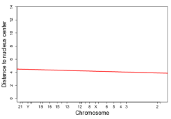
(a) Spherical Nucluei

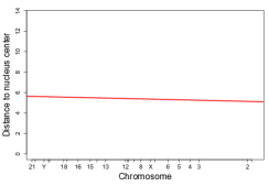
(b) Ellipsoidal Nuclei

Fig. 6: Scatter plots and regression lines for distances of ellipsoidal chromosome territories to nucleus center, for medium-sized nuclei. Horizontal axis is CT volume, vertical axis is distance to nucleus center.

In Table 3 we report the slopes of the regression line for all six scenarios. Interestingly, the negative trend is consistently weaker for flat ellipsoidal nuclei compared to spherical nuclei. Experimentalists report a preference for larger CTs to be on the periphery for ellipsoidal nuclei, while for spherical nuclei, the radial preferences are believed to be correlated with gene density.

Table 3: Slope of regression line for all six scenarios.

	small	medium	large
spherical	-0.0050562	-0.0029405	-0.0020672
ellipsoidal	-0.0047345	-0.0025045	-0.0018849

5.4 Radial preferences assuming heterologous CT groupings

Khalil et al. [9] showed that CTs tend to assemble in heterologous neighborhoods, causing the distances between homologous chromosome pairs to be larger in general than heterologous inter-CT distances. They discuss a number of possible explanations for this phenomenon, such as that heterologous neighborhoods act as a buffer zone in preventing inter-homologue recombination and protect against the loss of heterozygosity. The authors also analyze whether the radial preferences discussed in the previous subsection could explain the preference for arrangements with larger homologous inter-CT distances. Using simulations, they give a negative answer to this question.

In the following analysis, we invert the question, asking instead whether the preference for heterologous neighborhoods can explain the observed radial preferences. To investigate this question, we add penalties to our model to discourage the CTs in a homologous pair from being too close to each other. We solve the resulting formulation using a combination of Algorithm 1 for sphere packing with Algorithm 2 for ellipsoid packing.

We denote the set of index pairs $(i,j)$ corresponding to homologous chromosome pairs by $H$ and we introduce a new variable $\eta$ to capture the proximity of CTs in a homologous pair. Specifically, we define for each ellipsoid $i$ an enclosing sphere that is concentric with the ellipsoid $i$, with radius $\lambda$ times the maximum semi-axis length $r_{i}$ of the CT, where $\lambda\geq 1$ is a user-defined parameter. We define $\eta$ to be the maximal overlap of these enclosing spheres, over all homologous pairs, by adding constraints whose form is similar to (12b). We then add a penalty term $c\eta$ to the objective (where $c\geq 0$ is some penalty parameter), to obtain the following extension of formulation (22).

$$\min_{\xi,\eta,(c_{i},S_{i},\Sigma_{i}),i=1,2,\dotsc,N}\; \xi+c\eta$$ (52a)

subject to $$\xi\geq\hat{O}(c_{i},c_{j},\Sigma_{i},\Sigma_{j}), 1\leq i<j\leq N,$$ (52b)

$$\lambda(r_{i}-r_{j})-\lVert c_{i}-c_{j}\rVert_{2}\leq\eta, (i,j)\in H,$$ (52c)

$$\mathcal{E}_{i}\subset\mathcal{E}, i=1,2,\dots,N,$$ (52d)

$$\Sigma_{i}=S_{i}^{2},$$ (52e)

$$\mbox{semi-axes of }\mathcal{E}_{i}\mbox{ are }r_{i1},r_{i2},r_{i3}, i=1,2,\dots,N.$$ (52f)

We can relax this to obtain an extended formulation of (26). To solve, we extend Algorithm 2 by adding linearizations of the constraints (52b) to each subproblem, in the manner of (14b).

For our simulations, we choose $c=100$ and $\lambda=1.25$. As in Subsection 5.3, we generated about 100-200 trials by perturbing CT volumes and dimensions randomly around given mean values and using different random starting points. The screening procedure described in the previous subsection was applied to remove those trials with less competitive final objective values. Statistics for the final objectives are shown in Table 4. The large objective values in the first line of the table indicates that for small spherical nuclei, it was not possible to find solutions in which the homolog separation was enforced adequately. (The only trial that survived screening was one that violated these conditions significantly less than most others.) Among the other scenarios, only the medium spherical nucleus saw significant numbers of trials removed by screening. Here, most of the trials attained final objectives quite close to 1.90, while the others had significantly higher values. In the other four scenarios — small ellipsoidal, medium ellipsoidal, large spherical, and large ellipsoidal — proximity penalties for homologous pairs were not incurred, and final objective values were tightly clustered.

Table 4: Statistics for final objective values attained in the six scenarios in which homolog proximity is penalized, showing number of trials, means, and standard deviations, both before and after the screening step.

		Before Screening			After Screening
shape	vol ($\mu m^{3}$)	trials	mean	sd	trials	mean	sd
spherical	500	100	294.0617	46.8185	1	184.0292	0.0000
ellipsoidal	500	100	3.6556	0.2691	95	3.5987	0.0879
spherical	1000	200	15.0885	20.7260	114	1.8993	0.0833
ellipsoidal	1000	200	2.0088	0.5118	192	1.9060	0.0691
spherical	1600	100	0.4424	1.2293	94	0.1369	0.0213
ellipsoidal	1600	100	0.2752	0.8097	97	0.1343	0.0251

The convex relaxation of our problem that encourages separation of homologous CT pairs does less well in preserving the dimensions of the ellipsoids than the formulation considered in Section 5.3. For spherical nuclei 26 out of the 46 CTs for small nuclei experienced a relative change in the half-axes lengths of more than 10%. For the medium spherical nuclei it was in average 11 out of 46 and for the large spherical nuclei 17 out of 46. The statistics for the ellipsoidal nuclei were somewhat smaller: 12 for the small nuclei, 4 for the medium nuclei, and 9 for the large nuclei. On the small nuclei, the distortions can be explained by the tightness of space, while on large nuclei, the fact that all CTs can be fit without any overlap reduces the need for them to adopt their lowest-volume dimensions (which would achieve the prescribed semi-axis lengths).

Figure 7 contains scatter plots showing the mean volume of each CT (on the horizontal axis) plotted against the distance between the center of that CT and the nuclear center (on the vertical axis), for a medium-sized nucleus (volume of $1000$ $\mu m^{3}$) and for both spherical and flat ellipsoidal shapes. (As in Subsection 5.3, scatter plots for the large and small volume nuclei are similar, so we do not show them here.) Here the regression line shows a significant positive trend, meaning that the smaller ellipsoids tend to lie in the interior of the nucleus, while the larger ones prefer peripheral positions. Hence, by adding penalties on nearness of homologous pairs to the formulation, we are able to match the radial preferences observed in nature.

Another interesting observation, more evident in Figure 7(a), is that the X and Y chromosomes both lie closer to the nucleus center than their size would suggest. This makes sense, as these are the only two chromosomes not subject to the homologous-pair separation penalties.

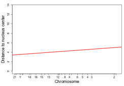
(a) Spherical Nuclei

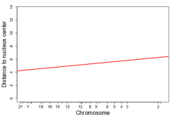
(b) Ellipsoidal Nuclei

Fig. 7: Scatter plots and regression lines for ellipsoidal chromosome territory distances to nucleus center, where penalties to enforce heterologous groupings are present in the objective. Horizontal axis is CT volume, vertical axis is distance to nucleus center.

In Table 5 we report the slopes of the regression line for all six size / shape scenarios considered in this section. These results highlight a significant difference between spherical and flat-ellipsoidal nuclei. The radial preference is consistently weaker for spherical nuclei than in flat-ellipsoidal nuclei.

Table 5: Slope of regression line for all six scenarios assuming heterologous CT groupings.

	small	medium	large
spherical	0.0031803	0.0078299	0.0072028
ellipsoidal	0.0081768	0.0102088	0.0145001

6 Discussion

We have described a bilevel optimization procedure for finding local solutions of the problem of packing spheres and ellipsoids in finite volumes, and used these procedures to model and analyze chromosome arrangement in cell nuclei. Semidefinite programming duality is used to obtain the sensitivity information needed to construct the approximation to the upper-level problem that is solved at each iteration of the trust-region procedure. Our convergence analysis takes place in a general setting in which the lower-level problems are semidefinite programs parametrized by their objective coefficient matrix; it is not confined to the specific form of the semidefinite programs arising from the S-procedure for overlapping ellipsoids. Thus it may be adaptable to other design problems involving parametrized systems that can be modeled by semidefinite programs.

In the CT packing application discussed in Section 5, we initially found that the arrangements observed experimentally could not be explained by the simple geometric principle of minimizing the maximum overlap. However, when we enhanced the model to capture the recently observed phenomenon of heterologous neighborhoods / homologous pair separation, the radial preferences observed in nature (in which larger CTs tended to lie further from the nuclear center) were recovered in our simulations. The homologous-pair-separation aspects of our model are governed by two positive parameters $c$ and $\lambda$; we reported results in Subsection 5.4 only for the values $c=100$ and $\lambda=1.25$. From an examination of Tables 3 and 5, we speculate that it would be possible to choose these parameters in such a way that the slope of the regression line for spherical nuclei would be approximately zero, while the corresponding slope for ellipsoidal nuclei would be positive. Such a result would be consistent with experimental observations that identify no clear radial preference for spherical nuclei, but a pronounced radial preference for ellipsoidal nuclei.

We obtained results on a limited but representative range of nuclei dimensions. In future work, we will explore CT configurations for a wider range of ellipsoidal shapes and sizes, corresponding to known dimensions of nuclei in different cell types. We will also enhance the model as further biological results are obtained, aiming to find biologically plausible, elementary principles that explain experimental observations (in the spirit of Occam’s Razor).

Appendix A Technical Results for Parametrized Semidefinite Programs

In this section we consider the following primal-dual pair of semidefinite programs that are parametrized by the primal objective term $C$:

$$\min_{X}\,\langle C,X\rangle\;\;\mbox{s.t.}\;\;\langle A_{i},X\rangle=b_{i},\;\;i=1,2,\dotsc,p,\;\;X\succeq 0,\\$$ (53)

$$\max_{\zeta,S}\,b^{T}\zeta\;\;\mbox{s.t.}\;\;\sum_{i=1}^{p}\zeta_{i}A_{i}+S=C,\;\;S\succeq 0.$$ (54)

We denote solutions of these problems by $X(C)$ and $(\zeta(C),S(C))$, respectively. (Our interest is in the application to the SDP pair (30), (34), but we have simplified the notation here.)

We show first that the solutions to (53) are uniformly bounded in a neighborhood of a $C$ for which a strictly feasible point for the dual (54) exists. The result is an almost immediate consequence of [17, Theorem 4.1].

Lemma 10.

Consider the primal-dual pair (53), (54) of semidefinite programs: Suppose that (53) is feasible (with feasible point $\hat{X}$), and that at some matrix $C_{0}\in S\makebox{\sf I R }^{n\times n}$, there exists a strictly feasible point $(\hat{\zeta},\hat{S})$ for (54), where the eigenvalues of $\hat{S}$ are bounded below by $\sigma>0$. Then there exists a constant $\delta>0$ such that for all matrices $C\in S\makebox{\sf I R }^{n\times n}$ with $\|C-C_{0}\|_{F}\leq\delta$, (53) has a nonempty solution set, and all solutions $X(C)$ are bounded as follows:

$$\|X(C)\|_{F}\leq\frac{2}{\sigma}(\langle\hat{X},\hat{S}\rangle+\delta\|\hat{X}\|_{F}).$$

Moreover the optimal values of the problems (53) and (54) are equal.

Proof.

We have for any $X$ feasible for the primal (note that the primal feasible region does not depend on $C$) that

$$\langle C,X\rangle =\langle C_{0},X\rangle+\langle C-C_{0},X\rangle$$

$$=\langle\sum_{i=1}^{p}\hat{\zeta}_{i}A_{i}+\hat{S},X\rangle+\langle C-C_{0},X\rangle$$

$$=b^{T}\hat{\zeta}+\langle\hat{S},X\rangle+\langle C-C_{0},X\rangle.$$

Since $b^{T}\hat{\zeta}$ is independent of $X$, we can obtain an equivalent to the primal problem by replacing its objective $\langle C,X\rangle$ by $\langle\hat{S}+C-C_{0},X\rangle$. Using the assumed feasible point $\hat{X}$ of (53) (note that there is no dependence of $\hat{X}$ on $C$), we can formulate (53) equivalently as follows:

$$\min_{X}\,\langle\hat{S}+C-C_{0},X\rangle\;\;\mbox{s.t.}\;\; \langle A_{i},X\rangle=b_{i},\;\;i=1,2,\dotsc,p,\;\;X\succeq 0,$$ (55a)

$$\langle\hat{S}+C-C_{0},X\rangle\leq\langle\hat{S}+C-C_{0},\hat{X}\rangle.$$ (55b)

By choosing $\delta\in(0,\sigma/2]$, we have that all eigenvalues of $\hat{S}+C-C_{0}$ are bounded below by $\sigma/2$. Hence from “Fact 14” of [17], we have that

$$\langle\hat{S}+C-C_{0},X\rangle\leq\langle\hat{S}+C-C_{0},\hat{X}\rangle\;\Rightarrow\;\|X\|_{F}\leq\frac{2}{\sigma}\langle\hat{S}+C-C_{0},\hat{X}\rangle\leq\frac{2}{\sigma}(\langle\hat{S},\hat{X}\rangle+\delta\|\hat{X}\|_{F}).$$

Hence, (55) involves the minimization of a continuous function over a nonempty compact set, so the solution set exists, and moreover, all solutions are bounded as claimed.

The last claim can be derived exactly as in [17, Theorem 4.1]. ∎

The next result examines the solution of a sequence of parametrized SDPs.

Theorem 11.

Given $A_{i}$, $i=1=1,2,\dotsc,p$ and $b\in\makebox{\sf I R }^{p}$ as in Lemma 10, such that (53) is feasible, let $\bar{C}\in S\makebox{\sf I R }^{n\times n}$ be such that there exists a strictly feasible point for (54) when $C=\bar{C}$. Consider a sequence $\{C_{k}\}$ with $C_{k}\in S\makebox{\sf I R }^{n\times n}$ and $C_{k}\to\bar{C}$. Then the following is true:

• There is a constant $\beta>0$ and index $K$ such that (53) with $C=C_{k}$ has nonempty solution set for all $k\geq K$, and $\|X(C_{k})\|_{F}\leq\beta$ for all such solutions.

• If $\{X(C_{k})\}$ is a sequence of solutions of (53) with $C=C_{k}$, then this sequence has at least one accumulation point, and all such accumulation points are solutions of (53) with $C=\bar{C}$.

Proof.

The first claim (i) is an immediate consequence of Lemma 10. For (ii), note that boundedness of $X(C_{k})$ ensures existence of accumulation points. Suppose that $\bar{X}$ is such a point and assume WLOG that $X(C_{k})\to\bar{X}$. Note first that $\bar{X}$ is feasible for (53) regardless of $C$. If $\bar{X}$ were not optimal for (53) with $C=\bar{C}$, then there would exist another feasible matrix $\tilde{X}$ with $\langle\bar{C},\tilde{X}\rangle<\langle\bar{C},\bar{X}\rangle$. But since

$$\lim_{k}\,\langle C_{k},\tilde{X}\rangle=\langle\bar{C},\tilde{X}\rangle<\langle\bar{C},\bar{X}\rangle=\lim_{k}\,\langle C_{k},X(C_{k})\rangle,$$

we have that $\langle C_{k},\tilde{X}\rangle<\langle C_{k},X(C_{k})\rangle$ for all $k$ sufficiently large, contradicting optimality of $X(C_{k})$. Hence (ii) is true. ∎

We next prove some elementary and useful facts about the value function of (53), which we denote by $t(C)$.

Lemma 12.

Suppose that (53) is feasible, and let $\bar{C}\in S\makebox{\sf I R }^{n\times n}$ be such that there exists a strictly feasible point for (54) when $C=\bar{C}$. Then there exists a neighborhood ${\cal N}$ of $\bar{C}$ within which the following claims are true.

• $t(\cdot)$ is a concave function.

• For all $C\in{\cal N}$ and all $\Delta C\in S\makebox{\sf I R }^{n\times n}$, we have

  $$t(C+\Delta C)\leq t(C)+\langle X(C),\Delta C\rangle,$$ (56)

  where $X(C)$ is any solution of (53).

• Any $X(C)$ that solves (53) belongs to the Clarke subdifferential of $t(\cdot)$ at $C$.

• $t(\cdot)$ is Lipschitz continuous in ${\cal N}$.

Proof.

The proof of (i) is elementary.

For (ii), note first from Lemma 10 that we can choose ${\cal N}$ so as to ensure that a solution $X(C)$ to (53) exists for all $C\in{\cal N}$. We have (denoting by $\Psi$ the feasible set for (53)) that

$$t(C+\Delta C)=\min_{X\in\Psi}\,\langle C+\Delta C,X\rangle\leq\langle C+\Delta C,X(C)\rangle=t(C)+\langle\Delta C,X(C)\rangle,$$

as required.

For (iii), note that (by taking the negative of the inequality (56)) $-X(C)$ is a subgradient of the convex function $(-t)(C)$, and so $-X(C)$ belongs to the Clarke subdifferential of $(-t)(C)$. It follows from [2, p. 128, Exercise 8(c)] (with $\lambda=-1$) that $X(C)$ belongs to the Clarke subdifferential of $t(C)$, as claimed.

For (iv), note from Lemma 10 that we can choose ${\cal N}$ such that $\|X(C)\|$ is uniformly bounded for all $C\in{\cal N}$ (by $\beta>0$, say). Denoting by $C_{1}$ and $C_{2}$ any two points in ${\cal N}$, we have from (56) that

$$t(C_{2}) \leq t(C_{1})+\langle X(C_{1}),C_{2}-C_{1}\rangle,$$

$$t(C_{1}) \leq t(C_{2})+\langle X(C_{2}),C_{1}-C_{2}\rangle.$$

Thus

$$|t(C_{1})-t(C_{2})|\leq\max\left(\|X(C_{1})\|,\|X(C_{2})\|\right)\|C_{1}-C_{2}\|\leq\beta\|C_{1}-C_{2}\|,$$

proving the Lipschitz property. ∎

Acknowledgments

We thank Saira Mian for helpful discussions about the application to chromosome arrangement in cell nuclei. We are grateful to the Institute for Mathematics and its Applications at the University of Minnesota for supporting visits by both authors while this research was conducted.

References

- [1] A. Bolzer, G. Kreth, I. Solovei, D. Koehler, K. Saracoglu, C. Fauth, S. Müller, R. Eils, C. Cremer, M. R. Speicher, and T. Cremer. Three-dimensional maps of all chromosomes in human male fibroblast nuclei and prometaphase rosettes. PLoS Biol., 3, 2005.
- [2] J. Borwein and A. S. Lewis. Convex Analysis and Nonlinear Optimization: Theory and Examples. CMS Books in Mathematics. Springer, 2000.
- [3] S. Boyd and L. Vandenberghe. Convex Optimization. Cambridge University Press, 2003.
- [4] F. H. Clarke. Optimization and Nonsmooth Analysis. John Wiley, New York, 1983.
- [5] T. Cremer and M. Cremer. Chromosome territories. Cold Spring Harb. Perspect. Biol., 2010.
- [6] A. Donev, I. Cisse, D. Sachs, E. A. Variano, F. H. Stillinger, R. Connelly, S. Torquato, and P. M. Chaikin. Improving the density of jammed disordered packings using ellipsoids. Science, 303:990–993, February 2004.
- [7] M. Grant and S. Boyd. CVX User’s Guide. Stanford University, version 1.22 edition, February 2012.
- [8] T. A. Hales. A proof of the Kepler conjecture. Annals of Mathematics, Second Series, 162(3):1065–1185, November 2005.
- [9] A. Khalil, J. L. Grant, L. B. Caddle, E. Atzema, K. D. Mills, and A. Arneodo. Chromosome territories have a highly nonspherical morphology and nonrandom positioning. Chromosome Res., 15:899–916, 2007.
- [10] B. D. Lubachevsky and R. L. Graham. Curved hexagonal packings of equal disks in a circle. Discrete and Computational Geometry, 18(2):179–194, June 2007.
- [11] N. V. Marella, S. Bhattacharya, L. Mukherjee, J. Xu, and R. Berezney. Cell type specific chromosome territory organization in the interphase nucleus of normal and cancer cells. J. Cell. Physiol., 221:130–138, 2009.
- [12] I. Müller, S. Boyle, R. H. Singer, W. A. Bickmore, and J. R. Chubb. Stable morphology, but dynamic internal reorganisation, of interphase human chromosomes in living cells. PLoS One, 5, 2010.
- [13] R. T. Rockafellar. Convex Analysis. Princeton University Press, Princeton, N.J., 1970.
- [14] C. A. Rogers. Packing and Covering, volume 54 of Cambridge Tracts in Mathematics and Mathematical Physics. Cambridge University Press, 1964.
- [15] H. Tanabe, S. Müller, M. Neusser, J. von Hase, E. Calcagno, M. Cremer, I. Solovei, C. Cremer, and T. Cremer. Evolutionary conservation of chromosome territory arrangements in cell nuclei from higher primates. Proc. Natl. Acad. Sci., 99:4424–4429, 2002.
- [16] A. Thue. Über die dichteste Zusammenstellung von kongruenten Kreisen in einer Ebene. Norske Vod. Selsk. Skr., 1:1–9, 1910.
- [17] M. J. Todd. Semidefinite optimization. Acta Numerica, 10:515–560, 2001.
- [18] M. J. Zeitz, L. Mukherjee, S. Bhattacharya, J. Xu, and R. Berezney. A probabilistic model for the arrangement of a subset of human chromosome territories in WI38 human fibroblasts. J. Cell. Physiol., 221:120–129, 2009.