Path integral Monte Carlo with importance sampling for excitons interacting with an arbitrary phonon bath

Sangwoo Shim    Alán Aspuru-Guzik Department of Chemistry and Chemical Biology, Harvard University, Cambridge, Massachusetts 02138, USA
Abstract

The reduced density matrix of excitons coupled to a phonon bath at a finite temperature is studied using the path integral Monte Carlo method. Appropriate choices of estimators and importance sampling schemes are crucial to the performance of the Monte Carlo simulation. We show that by choosing the population-normalized estimator for the reduced density matrix, an efficient and physically-meaningful sampling function can be obtained. In addition, the nonadiabatic phonon probability density is obtained as a byproduct during the sampling procedure. For importance sampling, we adopted the Metropolis-adjusted Langevin algorithm. The analytic expression for the gradient of the target probability density function associated with the population-normalized estimator cannot be obtained in closed form without a matrix power series. An approximated gradient that can be efficiently calculated is explored to achieve better computational scaling and efficiency. Application to a simple one-dimensional model system from the previous literature confirms the correctness of the method developed in this manuscript. The displaced harmonic model system within the single exciton manifold shows the numerically exact temperature dependence of the coherence and population of the excitonic system. The sampling scheme can be applied to an arbitrary anharmonic environment, such as multichromophoric systems embedded in the protein complex. The result of this study is expected to stimulate further development of real time propagation methods that satisfy the detailed balance condition for exciton populations.

I Introduction

Recent 2D non-linear spectroscopy experiments suggested the existence of long-lived quantum coherence during the electronic energy transfer process within the Fenna-Matthews-Olson complex of green sulfur bacteria, marine algae and plants even under physiological conditions Engel2007 ; Panitchayangkoon2010 ; Schlau-Cohen2012 ; Wong2012 ; Collini2010 ; Kolli2012 . These results attracted a large amount of attention from theoretical physicists and chemists. The energy transfer process usually has been modeled as the dynamics of excitons coupled to a phonon bath in thermal equilibrium within the single exciton manifold. This approximation leads to the famous spin-Boson Hamiltonian. The solution of this type of Hamiltonian has been studied extensively. For example, by assuming a certain relative magnitude between the reorganization energy and coupling terms, one can obtain quantum master equations valid in specific regimesForster1948 ; May2004 ; Redfield1957 . Another approximation, the Haken-Strobl-Reineker model works in both the coherent and incoherent regimes, but incorrectly converges to the high temperature limit in the long time even at the low temperature  Haken1972 ; Haken1973 . More recently, numerically exact approaches which interpolate both limits have been investigated and applied to many systems of interest. Two of the most popular methods are the hierarchical equation of motion  Ishizaki2005 ; Ishizaki2009a ; Ishizaki2009 and the quasiadiabatic path integral method Topaler1992 ; Makri1992 . These methods are being actively developed, improved, and applied to many systems of interests Zhu2011 .

Although having been successful in many applications, many of the models described above have assumed the phonon bath to be a set of independent harmonic oscillators and encode all the complexity of the bath environment in the spectral density, which is essentially a frequency dependent distribution of exciton-phonon coupling. However, for studying the anharmonic effects of a very sophisticated bath environment, like the protein complexes of photosynthesis, being able to directly include the atomistic details of the bath structure into the exciton dynamics has a distinct advantage. In other words, approaches that can evaluate the influence functional first suggested by Feynman and Vernon Feynman1963 have more straightforward descriptions and are applicable to arbitrary systems. Evaluation of the exact influence functional for arbitrary environment requires the simulation of the full quantum dynamics, which is still not practical with currently available computational resources. There have been several attempts to incorporate atomistic details of the large scale bath by combining the exciton dynamics and molecular dynamics simulations  Shim2012 ; Olbrich2010 ; Olbrich2011 . However, these theories are still in their early stages and the propagation scheme used does not satisfy some fundamental properties, like the detailed balance condition at finite temperature. In pursuit of more accurate theory, it is crucial to know the correct asymptotic behavior in the limit of infinite time. In this context, we decided to explore the numerically exact reduced density matrix in a finite temperature using path integral Monte Carlo Thirumalai1983 ; Allinger1986 ; Behrman1985 ; Cao1993 method. Recently, Moix et al applied path integral Monte Carlo for the equilibrium reduced density matrix of the FMO complex within the framework of open quantum systems Moix2012 .

II Theory

II.1 Path integral formulation of the reduced thermal density matrix

We want to evaluate the reduced density matrix of an excitonic system coupled to phonons on arbitrary Born-Oppenheimer surfaces at a finite temperature. For photosynthetic energy transfer, we usually restrict the excitons to be within the single exciton manifold because at normal light intensity, in average, one photon is present at a given time in the complexes of interest. However, the formulation itself is not limited to the single exciton manifold. The Hamiltonian operator for such a system can be written as

H^^𝐻\displaystyle\hat{H} =m𝑑𝑹[Vm(𝑹)Vg(𝑹)]|mm||𝑹𝑹|+mn𝑑𝑹Jmn(𝑹)|mn||𝑹𝑹|H^exc=H^S+H^SBabsentsubscriptsubscript𝑚tensor-producttensor-productdifferential-d𝑹delimited-[]subscript𝑉𝑚𝑹subscript𝑉𝑔𝑹ket𝑚bra𝑚ket𝑹quantum-operator-product𝑹subscript𝑚𝑛differential-d𝑹subscript𝐽𝑚𝑛𝑹𝑚bra𝑛ket𝑹bra𝑹subscript^𝐻excsubscript^𝐻𝑆subscript^𝐻𝑆𝐵\displaystyle=\underbrace{\sum_{m}\int d\bm{R}\ \left[V_{m}(\bm{R})-V_{g}(\bm{R})\right]|m\rangle\langle m|\otimes|\bm{R}\rangle\langle\bm{R}|+\sum_{m\neq n}\int d\bm{R}\ J_{mn}(\bm{R})|m\rangle\langle n|\otimes|\bm{R}\rangle\langle\bm{R}|}_{\hat{H}_{\rm exc}=\hat{H}_{S}+\hat{H}_{SB}}
+|𝟏𝟏|[T^+𝑑𝑹Vg(𝑹)|𝑹𝑹|]H^B.subscripttensor-productket1bra1delimited-[]^𝑇differential-d𝑹subscript𝑉𝑔𝑹ket𝑹bra𝑹subscript^𝐻𝐵\displaystyle+\underbrace{|\bm{1}\rangle\langle\bm{1}|\otimes\left[\hat{T}+\int d\bm{R}\ V_{g}(\bm{R})|\bm{R}\rangle\langle\bm{R}|\right]}_{\hat{H}_{B}}. (1)

The Hamiltonian was written in terms of the diabatic basis |m,𝑹|m|𝑹ket𝑚𝑹tensor-productket𝑚ket𝑹|m,\bm{R}\rangle\equiv|m\rangle\otimes|\bm{R}\rangle, where m𝑚m is the index for the exciton state and R𝑅R is the phonon coordinate. Vg(𝑹)subscript𝑉𝑔𝑹V_{g}(\bm{R}) is the potential energy surface (PES) of the phonons in the electronic ground state and Vm(𝑹)subscript𝑉𝑚𝑹V_{m}(\bm{R}) is the PES of the phonons in the m𝑚mth exciton state. T^^𝑇\hat{T} is the kinetic operator of the phonons defined as T^=2212,^𝑇superscriptPlanck-constant-over-2-pi22superscript1superscript2\hat{T}=-\frac{\hbar^{2}}{2}\mathcal{M}^{-1}\nabla^{2}, where \mathcal{M} is the mass tensor of the phonons. This expression is generally applicable to any molecular system with multiple potential energy surfaces. The reduced thermal density matrix ρSsubscript𝜌𝑆\rho_{S} is defined as the partial trace of the full thermal density matrix with respect to the bath degrees of freedom:

ρSsubscript𝜌𝑆\displaystyle\rho_{S} =1Z(β)TrBexp(βH^)absent1𝑍𝛽subscriptTrB𝛽^𝐻\displaystyle=\frac{1}{Z(\beta)}{\rm Tr_{B}}\exp\left(-\beta\hat{H}\right)
=1Z(β)𝑑𝑹0𝑹0|exp(βH^)|𝑹0,absent1𝑍𝛽differential-dsubscript𝑹0quantum-operator-productsubscript𝑹0𝛽^𝐻subscript𝑹0\displaystyle=\frac{1}{Z(\beta)}\int d\bm{R}_{0}\ \langle\bm{R}_{0}|\exp\left(-\beta\hat{H}\right)|\bm{R}_{0}\rangle, (2)

where Z(β)𝑍𝛽Z(\beta) is the partition function of the total system. We proceed by relying on the following identity:

𝑹0|exp(βH^)|𝑹0quantum-operator-productsubscript𝑹0𝛽^𝐻subscript𝑹0\displaystyle\langle\bm{R}_{0}|\exp(-\beta\hat{H})|\bm{R}_{0}\rangle =𝑹0|{exp(βH^M)}M|𝑹0absentquantum-operator-productsubscript𝑹0superscript𝛽^𝐻𝑀𝑀subscript𝑹0\displaystyle=\langle\bm{R}_{0}|\left\{\exp\left(-\frac{\beta\hat{H}}{M}\right)\right\}^{M}|\bm{R}_{0}\rangle
=𝑑𝑹1𝑑𝑹2𝑑𝑹M1absentdifferential-dsubscript𝑹1differential-dsubscript𝑹2differential-dsubscript𝑹𝑀1\displaystyle=\int d\bm{R}_{1}\int d\bm{R}_{2}\cdots\int d\bm{R}_{M-1}
×𝑹0|exp(βH^M)|𝑹M1𝑹M1|exp(βH^M)|𝑹M2absentquantum-operator-productsubscript𝑹0𝛽^𝐻𝑀subscript𝑹𝑀1quantum-operator-productsubscript𝑹𝑀1𝛽^𝐻𝑀subscript𝑹𝑀2\displaystyle\ \times\langle\bm{R}_{0}|\exp\left(-\frac{\beta\hat{H}}{M}\right)|\bm{R}_{M-1}\rangle\langle\bm{R}_{M-1}|\exp\left(-\frac{\beta\hat{H}}{M}\right)|\bm{R}_{M-2}\rangle\cdots
×𝑹2|exp(βH^M)|𝑹1𝑹1|exp(βH^M)|𝑹0.absentquantum-operator-productsubscript𝑹2𝛽^𝐻𝑀subscript𝑹1quantum-operator-productsubscript𝑹1𝛽^𝐻𝑀subscript𝑹0\displaystyle\ \times\langle\bm{R}_{2}|\exp\left(-\frac{\beta\hat{H}}{M}\right)|\bm{R}_{1}\rangle\langle\bm{R}_{1}|\exp\left(-\frac{\beta\hat{H}}{M}\right)|\bm{R}_{0}\rangle. (3)

For any positive integer M𝑀M, the expression above is exact. When the Trotter decomposition is applied, an imaginary timestep τβM𝜏𝛽Planck-constant-over-2-pi𝑀\tau\equiv\frac{\beta\hbar}{M} is usually defined for convenience. Then, the thermal density matrix can be interpreted as an imaginary time evolution. In the limit of an infinitesimal imaginary timestep, the Trotter decomposition converges to the exact result,

𝑹1|exp(βH^M)|𝑹0quantum-operator-productsubscript𝑹1𝛽^𝐻𝑀subscript𝑹0\displaystyle\langle\bm{R}_{1}|\exp\left(-\frac{\beta\hat{H}}{M}\right)|\bm{R}_{0}\rangle =𝑹1|exp(τH^/)|𝑹0absentquantum-operator-productsubscript𝑹1𝜏^𝐻Planck-constant-over-2-pisubscript𝑹0\displaystyle=\langle\bm{R}_{1}|\exp\left(-\tau\hat{H}/\hbar\right)|\bm{R}_{0}\rangle
=𝑹1|eτH^exc/2eτH^B/eτH^exc/2|𝑹0+O(τ3)absentquantum-operator-productsubscript𝑹1superscript𝑒𝜏subscript^𝐻exc2Planck-constant-over-2-pisuperscript𝑒𝜏subscript^𝐻𝐵Planck-constant-over-2-pisuperscript𝑒𝜏subscript^𝐻exc2Planck-constant-over-2-pisubscript𝑹0𝑂superscript𝜏3\displaystyle=\langle\bm{R}_{1}|e^{-\tau\hat{H}_{\rm exc}/2\hbar}e^{-\tau\hat{H}_{B}/\hbar}e^{-\tau\hat{H}_{\rm exc}/2\hbar}|\bm{R}_{0}\rangle+O(\tau^{3})
=𝑑𝑹2𝑑𝑹3𝑹1|eτH^exc/2|𝑹3absentdifferential-dsubscript𝑹2differential-dsubscript𝑹3quantum-operator-productsubscript𝑹1superscript𝑒𝜏subscript^𝐻exc2Planck-constant-over-2-pisubscript𝑹3\displaystyle=\int d\bm{R}_{2}\int d\bm{R}_{3}\ \langle\bm{R}_{1}|e^{-\tau\hat{H}_{\rm exc}/2\hbar}|\bm{R}_{3}\rangle
×𝑹3|eτH^B/|𝑹2𝑹2|eτH^exc/2|𝑹0+O(τ3).absentquantum-operator-productsubscript𝑹3superscript𝑒𝜏subscript^𝐻𝐵Planck-constant-over-2-pisubscript𝑹2quantum-operator-productsubscript𝑹2superscript𝑒𝜏subscript^𝐻exc2Planck-constant-over-2-pisubscript𝑹0𝑂superscript𝜏3\displaystyle\ \times\langle\bm{R}_{3}|e^{-\tau\hat{H}_{B}/\hbar}|\bm{R}_{2}\rangle\langle\bm{R}_{2}|e^{-\tau\hat{H}_{\rm exc}/2\hbar}|\bm{R}_{0}\rangle+O(\tau^{3}). (4)

Subsequently, we will recast the system part of H^excsubscript^𝐻exc\hat{H}_{\rm exc} as a single matrix to simplify the notation,

H^excsubscript^𝐻exc\displaystyle\hat{H}_{\rm exc} =m,n𝑑𝑹Emn(𝑹)|mn||𝑹𝑹|,absentsubscript𝑚𝑛tensor-productdifferential-d𝑹subscript𝐸𝑚𝑛𝑹ket𝑚bra𝑛ket𝑹bra𝑹\displaystyle=\sum_{m,n}\int d\bm{R}\ E_{mn}(\bm{R})|m\rangle\langle n|\otimes|\bm{R}\rangle\langle\bm{R}|,
Emm(𝑹)subscript𝐸𝑚𝑚𝑹\displaystyle E_{mm}(\bm{R}) ={Vm(𝑹)Vg(𝑹)form=n,Jmn(𝑹)formn.absentcasessubscript𝑉𝑚𝑹subscript𝑉𝑔𝑹𝑓𝑜𝑟𝑚𝑛subscript𝐽𝑚𝑛𝑹𝑓𝑜𝑟𝑚𝑛\displaystyle=\left\{\begin{array}[]{rcr}V_{m}(\bm{R})-V_{g}(\bm{R})&for&m=n,\\ J_{mn}(\bm{R})&for&m\neq n.\end{array}\right. (7)

With the single exciton manifold assumption, Emmsubscript𝐸𝑚𝑚E_{mm} corresponds to the optical gap of the m𝑚m-th site. Now, the three terms in the integrand of the Eq. II.1 can be written without Dirac notation,

𝑹1|eτH^exc/2|𝑹3quantum-operator-productsubscript𝑹1superscript𝑒𝜏subscript^𝐻exc2Planck-constant-over-2-pisubscript𝑹3\displaystyle\langle\bm{R}_{1}|e^{-\tau\hat{H}_{\rm exc}/2\hbar}|\bm{R}_{3}\rangle =δ(𝑹1𝑹3)eτE(𝑹3)/2,absent𝛿subscript𝑹1subscript𝑹3superscript𝑒𝜏𝐸subscript𝑹32Planck-constant-over-2-pi\displaystyle=\delta(\bm{R}_{1}-\bm{R}_{3})e^{-\tau E(\bm{R}_{3})/2\hbar},
𝑹3|eτH^B/|𝑹2quantum-operator-productsubscript𝑹3superscript𝑒𝜏subscript^𝐻𝐵Planck-constant-over-2-pisubscript𝑹2\displaystyle\langle\bm{R}_{3}|e^{-\tau\hat{H}_{B}/\hbar}|\bm{R}_{2}\rangle =(4πτ|λ|)1/2eτVg(𝑹3)/2e(𝑹3𝑹2)Tλ1(𝑹3𝑹2)/4τeτVg(𝑹2)/2+O(τ3),absentsuperscript4𝜋𝜏𝜆12superscript𝑒𝜏subscript𝑉𝑔subscript𝑹32Planck-constant-over-2-pisuperscript𝑒superscriptsubscript𝑹3subscript𝑹2𝑇superscript𝜆1subscript𝑹3subscript𝑹24𝜏superscript𝑒𝜏subscript𝑉𝑔subscript𝑹22Planck-constant-over-2-pi𝑂superscript𝜏3\displaystyle=(4\pi\tau|\lambda|)^{-1/2}e^{-\tau V_{g}(\bm{R}_{3})/2\hbar}e^{-(\bm{R}_{3}-\bm{R}_{2})^{T}\lambda^{-1}(\bm{R}_{3}-\bm{R}_{2})/4\tau}e^{-\tau V_{g}(\bm{R}_{2})/2\hbar}+O(\tau^{3}),
𝑹2|eτH^exc/2|𝑹0quantum-operator-productsubscript𝑹2superscript𝑒𝜏subscript^𝐻exc2Planck-constant-over-2-pisubscript𝑹0\displaystyle\langle\bm{R}_{2}|e^{-\tau\hat{H}_{\rm exc}/2\hbar}|\bm{R}_{0}\rangle =δ(𝑹2𝑹0)eτE(𝑹0)/2,absent𝛿subscript𝑹2subscript𝑹0superscript𝑒𝜏𝐸subscript𝑹02Planck-constant-over-2-pi\displaystyle=\delta(\bm{R}_{2}-\bm{R}_{0})e^{-\tau E(\bm{R}_{0})/2\hbar}, (8)

where λ12𝜆Planck-constant-over-2-pisuperscript12\lambda\equiv\frac{\hbar\mathcal{M}^{-1}}{2}. By the Eq. II.1 and Eq. II.1,

𝑹1|exp(βH^M)|𝑹0quantum-operator-productsubscript𝑹1𝛽^𝐻𝑀subscript𝑹0\displaystyle\langle\bm{R}_{1}|\exp\left(-\frac{\beta\hat{H}}{M}\right)|\bm{R}_{0}\rangle =(4πτ|λ|)1/2eτVg(𝑹1)/2e(𝑹1𝑹0)Tλ1(𝑹1𝑹0)/4τeτVg(𝑹0)/2absentsuperscript4𝜋𝜏𝜆12superscript𝑒𝜏subscript𝑉𝑔subscript𝑹12Planck-constant-over-2-pisuperscript𝑒superscriptsubscript𝑹1subscript𝑹0𝑇superscript𝜆1subscript𝑹1subscript𝑹04𝜏superscript𝑒𝜏subscript𝑉𝑔subscript𝑹02Planck-constant-over-2-pi\displaystyle=(4\pi\tau|\lambda|)^{-1/2}e^{-\tau V_{g}(\bm{R}_{1})/2\hbar}e^{-(\bm{R}_{1}-\bm{R}_{0})^{T}\lambda^{-1}(\bm{R}_{1}-\bm{R}_{0})/{4\tau}}e^{-\tau V_{g}(\bm{R}_{0})/2\hbar}
×eτE(𝑹1)/2eτE(𝑹0)/2+O(τ3).absentsuperscript𝑒𝜏𝐸subscript𝑹12Planck-constant-over-2-pisuperscript𝑒𝜏𝐸subscript𝑹02Planck-constant-over-2-pi𝑂superscript𝜏3\displaystyle\ \times e^{-\tau E(\bm{R}_{1})/2\hbar}e^{-\tau E(\bm{R}_{0})/2\hbar}+O(\tau^{3}). (9)

Note that Eq. II.1 is a matrix with the same dimension as the  reduced density matrix of the system. Substituting Eq. II.1 to Eq. II.1, we obtain

ρSsubscript𝜌𝑆\displaystyle\rho_{S} =1Z(β)𝑑𝑹0𝑑𝑹1𝑑𝑹M1absent1𝑍𝛽differential-dsubscript𝑹0differential-dsubscript𝑹1differential-dsubscript𝑹𝑀1\displaystyle=\frac{1}{Z(\beta)}\int d\bm{R}_{0}\int d\bm{R}_{1}\cdots\int d\bm{R}_{M-1}
×eτE(𝑹0)/2eτE(𝑹M1)/eτE(𝑹1)/eτE(𝑹0)/2absentsuperscript𝑒𝜏𝐸subscript𝑹02Planck-constant-over-2-pisuperscript𝑒𝜏𝐸subscript𝑹𝑀1Planck-constant-over-2-pisuperscript𝑒𝜏𝐸subscript𝑹1Planck-constant-over-2-pisuperscript𝑒𝜏𝐸subscript𝑹02Planck-constant-over-2-pi\displaystyle\ \times e^{-\tau E(\bm{R}_{0})/2\hbar}e^{-\tau E(\bm{R}_{M-1})/\hbar}\cdots e^{-\tau E(\bm{R}_{1})/\hbar}e^{-\tau E(\bm{R}_{0})/2\hbar}
×eτVg(𝑹0)/eτVg(𝑹1)/eτVg(𝑹M1)/absentsuperscript𝑒𝜏subscript𝑉𝑔subscript𝑹0Planck-constant-over-2-pisuperscript𝑒𝜏subscript𝑉𝑔subscript𝑹1Planck-constant-over-2-pisuperscript𝑒𝜏subscript𝑉𝑔subscript𝑹𝑀1Planck-constant-over-2-pi\displaystyle\times e^{-\tau V_{g}(\bm{R}_{0})/\hbar}e^{-\tau V_{g}(\bm{R}_{1})/\hbar}\cdots e^{-\tau V_{g}(\bm{R}_{M-1})/\hbar}
×e(𝑹0𝑹M1)Tλ1(𝑹0𝑹M1)/4τe(𝑹M1𝑹M2)Tλ1(𝑹M1𝑹M2)/4τabsentsuperscript𝑒superscriptsubscript𝑹0subscript𝑹𝑀1𝑇superscript𝜆1subscript𝑹0subscript𝑹𝑀14𝜏superscript𝑒superscriptsubscript𝑹𝑀1subscript𝑹𝑀2𝑇superscript𝜆1subscript𝑹𝑀1subscript𝑹𝑀24𝜏\displaystyle\times e^{-(\bm{R}_{0}-\bm{R}_{M-1})^{T}\lambda^{-1}(\bm{R}_{0}-\bm{R}_{M-1})/4\tau}e^{-(\bm{R}_{M-1}-\bm{R}_{M-2})^{T}\lambda^{-1}(\bm{R}_{M-1}-\bm{R}_{M-2})/4\tau}
××e(𝑹1𝑹0)Tλ1(𝑹1𝑹0)/4τabsentsuperscript𝑒superscriptsubscript𝑹1subscript𝑹0𝑇superscript𝜆1subscript𝑹1subscript𝑹04𝜏\displaystyle\ \times\cdots\times e^{-(\bm{R}_{1}-\bm{R}_{0})^{T}\lambda^{-1}(\bm{R}_{1}-\bm{R}_{0})/4\tau}
=𝑑𝑹0𝑑𝑹1𝑑𝑹M1absentdifferential-dsubscript𝑹0differential-dsubscript𝑹1differential-dsubscript𝑹𝑀1\displaystyle=\int d\bm{R}_{0}\int d\bm{R}_{1}\cdots\int d\bm{R}_{M-1}
×KZ(β)eτE(𝑹0)/2eτE(𝑹M1)/eτE(𝑹1)/eτE(𝑹0)/2ρPIMC(𝑹0,,𝑹M1)absentsubscript𝐾𝑍𝛽superscript𝑒𝜏𝐸subscript𝑹02Planck-constant-over-2-pisuperscript𝑒𝜏𝐸subscript𝑹𝑀1Planck-constant-over-2-pisuperscript𝑒𝜏𝐸subscript𝑹1Planck-constant-over-2-pisuperscript𝑒𝜏𝐸subscript𝑹02Planck-constant-over-2-pisubscript𝜌PIMCsubscript𝑹0subscript𝑹𝑀1\displaystyle\ \times\underbrace{\frac{K}{Z(\beta)}e^{-\tau E(\bm{R}_{0})/2\hbar}e^{-\tau E(\bm{R}_{M-1})/\hbar}\cdots e^{-\tau E(\bm{R}_{1})/\hbar}e^{-\tau E(\bm{R}_{0})/2\hbar}}_{\rho_{\rm PIMC}(\bm{R}_{0},\cdots,\bm{R}_{M-1})}
×1KeβVPIMC(𝑹0,𝑹1,,𝑹M1)fg(𝑹0,,𝑹M1),absentsubscript1𝐾superscript𝑒𝛽subscript𝑉PIMCsubscript𝑹0subscript𝑹1subscript𝑹𝑀1subscript𝑓𝑔subscript𝑹0subscript𝑹𝑀1\displaystyle\ \times\underbrace{\frac{1}{K}e^{-\beta V_{\rm PIMC}(\bm{R}_{0},\bm{R}_{1},\cdots,\bm{R}_{M-1})}}_{f_{g}(\bm{R}_{0},\cdots,\bm{R}_{M-1})}, (10)

where,

VPIMC(𝑹0,𝑹1,,𝑹M1)subscript𝑉PIMCsubscript𝑹0subscript𝑹1subscript𝑹𝑀1\displaystyle V_{\rm PIMC}(\bm{R}_{0},\bm{R}_{1},\cdots,\bm{R}_{M-1}) =1Mi=0M1Vg(𝑹i)absent1𝑀superscriptsubscript𝑖0𝑀1subscript𝑉𝑔subscript𝑹𝑖\displaystyle=\frac{1}{M}\sum_{i=0}^{M-1}V_{g}(\bm{R}_{i})
+i=0M1M2β22{𝑹i𝑹mod(i+1,M)}T{𝑹i𝑹mod(i+1,M)}.superscriptsubscript𝑖0𝑀1𝑀2superscript𝛽2superscriptPlanck-constant-over-2-pi2superscriptsubscript𝑹𝑖subscript𝑹mod𝑖1𝑀𝑇subscript𝑹𝑖subscript𝑹mod𝑖1𝑀\displaystyle\ +\sum_{i=0}^{M-1}\frac{M}{2\beta^{2}\hbar^{2}}\{\bm{R}_{i}-\bm{R}_{{\rm mod}(i+1,M)}\}^{T}\mathcal{M}\{\bm{R}_{i}-\bm{R}_{{\rm mod}(i+1,M)}\}. (11)

The expressions above show that the reduced thermal density matrix ρSsubscript𝜌𝑆\rho_{S} can be evaluated as an expectation value of ρPIMC(𝑹0,,𝑹M1)subscript𝜌PIMCsubscript𝑹0subscript𝑹𝑀1\rho_{\rm PIMC}(\bm{R}_{0},\cdots,\bm{R}_{M-1}) where the joint probability density function of the M𝑀M N𝑁N-dimensional random variables (𝑹0,,𝑹M1)subscript𝑹0subscript𝑹𝑀1(\bm{R}_{0},\cdots,\bm{R}_{M-1}) is fgsubscript𝑓𝑔f_{g}. This type of multidimensional integral can be efficiently evaluated using Monte Carlo integration. Because fg(𝑹0,,𝑹M1)subscript𝑓𝑔subscript𝑹0subscript𝑹𝑀1f_{g}(\bm{R}_{0},\cdots,\bm{R}_{M-1}) is invariant to cyclic permutation of the phonon coordinate, usually the averaged estimator ρPIMCsubscript𝜌PIMC\rho_{\rm PIMC} over the cyclic permutation is used in the actual Monte Carlo evaluation:

ρPIMC¯=1Mi=0M1ρPIMC(𝑹i,𝑹mod(i+1,M),,𝑹mod(i+M1,M)).subscript𝜌¯PIMC1𝑀superscriptsubscript𝑖0𝑀1subscript𝜌PIMCsubscript𝑹𝑖subscript𝑹mod𝑖1𝑀subscript𝑹mod𝑖𝑀1𝑀\displaystyle\rho_{\rm\overline{PIMC}}=\frac{1}{M}\sum_{i=0}^{M-1}\rho_{\rm PIMC}(\bm{R}_{i},\bm{R}_{{\rm mod}(i+1,M)},\cdots,\bm{R}_{{\rm mod}(i+M-1,M)}). (12)

II.2 Population-normalized estimator and importance sampling

In the previous approach described in Eq. II.1, the phonon coordinates are sampled according the electronic ground state PES. The estimator should converge to the target quantity in the long time limit, taking into account the discretization error. As long as fg(𝑹0,,𝑹M1)subscript𝑓𝑔subscript𝑹0subscript𝑹𝑀1f_{g}(\bm{R}_{0},\cdots,\bm{R}_{M-1}) is positive definite everywhere in the phonon space, the sampling efficiency depends on the selection of the probability density. Obviously, the actual distribution of the phonon coordinate depends heavily on the excited state PES. Therefore, the Monte Carlo points coordinates sampled according to the reduced dynamics of the bath by taking the partial trace with respect to the exciton degrees of freedom, as explored in multiple surface path integral Monte Carlo approaches, are expected to give the better estimates. This choice of the probability density reweights the estimator in the following way:

fI(𝑹0,,𝑹M1)subscript𝑓𝐼subscript𝑹0subscript𝑹𝑀1\displaystyle f_{I}(\bm{R}_{0},\cdots,\bm{R}_{M-1}) =TrS[ρPIMC¯(𝑹0,,𝑹M1)]fg(𝑹0,,𝑹M1),absentsubscriptTrSdelimited-[]subscript𝜌¯PIMCsubscript𝑹0subscript𝑹𝑀1subscript𝑓𝑔subscript𝑹0subscript𝑹𝑀1\displaystyle={\rm Tr_{S}}\left[\rho_{\rm\overline{PIMC}}(\bm{R}_{0},\cdots,\bm{R}_{M-1})\right]f_{g}(\bm{R}_{0},\cdots,\bm{R}_{M-1}),
ρI(𝑹0,,𝑹M1)subscript𝜌𝐼subscript𝑹0subscript𝑹𝑀1\displaystyle\rho_{I}(\bm{R}_{0},\cdots,\bm{R}_{M-1}) =ρPIMC¯(𝑹0,,𝑹M1)TrS[ρPIMC¯(𝑹0,,𝑹M1)].absentsubscript𝜌¯PIMCsubscript𝑹0subscript𝑹𝑀1subscriptTrSdelimited-[]subscript𝜌¯PIMCsubscript𝑹0subscript𝑹𝑀1\displaystyle=\frac{\rho_{\rm\overline{PIMC}}(\bm{R}_{0},\cdots,\bm{R}_{M-1})}{{\rm Tr_{S}}\left[\rho_{\rm\overline{PIMC}}(\bm{R}_{0},\cdots,\bm{R}_{M-1})\right]}. (13)

In the expression above, we call ρI(𝑹0,,𝑹M1)subscript𝜌𝐼subscript𝑹0subscript𝑹𝑀1\rho_{I}(\bm{R}_{0},\cdots,\bm{R}_{M-1}) the population normalized estimator for the reduced density matrix because the sum of its populations is always constrained to be 1. The effective energy gap term of 1βlogTrρPIMC¯(𝑹0,,𝑹M1)1𝛽Trsubscript𝜌¯PIMCsubscript𝑹0subscript𝑹𝑀1-\frac{1}{\beta}\log{\rm Tr}\rho_{\rm\overline{PIMC}}(\bm{R}_{0},\cdots,\bm{R}_{M-1}) was added to the Eq. II.1 to enable the phonons follow the excited state dynamics depending on the exciton state ρS.subscript𝜌𝑆\rho_{S}. For the estimator of the reduced density matrix in Eq. II.1, the normalization must obtained by the estimates of its diagonal elements, leading to more uncertainties in the coherence. However, the population-normalized estimator preserves the correct normalization by construction, and does not suffer from any additional uncertainty.

Local gradient information can improve the efficiency and scaling of the sampling procedure by means of a gradient-based approach such as the Metropolis-adjusted Langevin algorithm (MALA). Robert2004 ; Pillai2011 However, the exact closed form of the gradient of the effective energy gap term, logTrSρPIMC¯(𝑹0,,𝑹M1)subscriptTrSsubscript𝜌¯PIMCsubscript𝑹0subscript𝑹𝑀1\log{\rm Tr_{S}}\rho_{\rm\overline{PIMC}}(\bm{R}_{0},\cdots,\bm{R}_{M-1}) can only be expressed as a function of a power series of matrices. Nevertheless, with the following approximation:

k=0nAkBAnkk=0n12n(nk)AkBAnk,superscriptsubscript𝑘0𝑛superscript𝐴𝑘𝐵superscript𝐴𝑛𝑘superscriptsubscript𝑘0𝑛1superscript2𝑛binomial𝑛𝑘superscript𝐴𝑘𝐵superscript𝐴𝑛𝑘\displaystyle\sum_{k=0}^{n}A^{k}BA^{n-k}\approx\sum_{k=0}^{n}\frac{1}{2^{n}}{\binom{n}{k}}A^{k}BA^{n-k}, (14)

an accurate approximated of the gradient can be obtained and employed in the sampling procedure,

RijlogTrS[ρPIMC¯(𝑹0,,𝑹M1)]subscript𝑅𝑖𝑗subscriptTrSdelimited-[]subscript𝜌¯PIMCsubscript𝑹0subscript𝑹𝑀1\displaystyle\frac{\partial}{\partial R_{ij}}\log{\rm Tr_{S}}\left[\rho_{\rm\overline{PIMC}}(\bm{R}_{0},\cdots,\bm{R}_{M-1})\right] =TrS[RijρPIMC¯(𝑹0,,𝑹M1)]TrS[ρPIMC¯(𝑹0,,𝑹M1)]absentsubscriptTrSdelimited-[]subscript𝑅𝑖𝑗subscript𝜌¯PIMCsubscript𝑹0subscript𝑹𝑀1subscriptTrSdelimited-[]subscript𝜌¯PIMCsubscript𝑹0subscript𝑹𝑀1\displaystyle=\frac{{\rm Tr_{S}}\left[\frac{\partial}{\partial R_{ij}}\rho_{\rm\overline{PIMC}}(\bm{R}_{0},\cdots,\bm{R}_{M-1})\right]}{{\rm Tr_{S}}\left[\rho_{\rm\overline{PIMC}}(\bm{R}_{0},\cdots,\bm{R}_{M-1})\right]}
TrS[τ2E(𝑹i)RijρPIMC¯(𝑹0,,𝑹M1)]TrS[ρPIMC¯(𝑹0,,𝑹M1)],absentsubscriptTrSdelimited-[]𝜏2Planck-constant-over-2-pi𝐸subscript𝑹𝑖subscript𝑅𝑖𝑗subscript𝜌¯PIMCsubscript𝑹0subscript𝑹𝑀1subscriptTrSdelimited-[]subscript𝜌¯PIMCsubscript𝑹0subscript𝑹𝑀1\displaystyle\approx\frac{{\rm Tr_{S}}\left[-\frac{\tau}{2\hbar}\frac{\partial E(\bm{R}_{i})}{\partial{R}_{ij}}\rho_{\rm\overline{PIMC}}(\bm{R}_{0},\cdots,\bm{R}_{M-1})\right]}{{\rm Tr_{S}}\left[\rho_{\rm\overline{PIMC}}(\bm{R}_{0},\cdots,\bm{R}_{M-1})\right]},
ilogfg(𝑹0,,𝑹M1)subscript𝑖subscript𝑓𝑔subscript𝑹0subscript𝑹𝑀1\displaystyle\nabla_{i}\log f_{g}(\bm{R}_{0},\cdots,\bm{R}_{M-1}) =βMiVg(𝑹i)absent𝛽𝑀subscript𝑖subscript𝑉𝑔subscript𝑹𝑖\displaystyle=-\frac{\beta}{M}\nabla_{i}V_{g}(\bm{R}_{i})
+M2β2(𝑹mod(i+1,M)+𝑹mod(i1,M)2𝑹i),𝑀2𝛽superscriptPlanck-constant-over-2-pi2subscript𝑹mod𝑖1𝑀subscript𝑹mod𝑖1𝑀2subscript𝑹𝑖\displaystyle\ +\frac{M}{2\beta\hbar^{2}}\mathcal{M}(\bm{R}_{{\rm mod}(i+1,M)}+\bm{R}_{{\rm mod}(i-1,M)}-2\bm{R}_{i}),
μi(𝑹0,,𝑹M1)subscript𝜇𝑖subscript𝑹0subscript𝑹𝑀1\displaystyle\mu_{i}(\bm{R}_{0},\cdots,\bm{R}_{M-1}) =TrS[τ2E(𝑹i)RijρPIMC¯(𝑹0,,𝑹M1)]TrS[ρPIMC¯(𝑹0,,𝑹M1)]absentsubscriptTrSdelimited-[]𝜏2Planck-constant-over-2-pi𝐸subscript𝑹𝑖subscript𝑅𝑖𝑗subscript𝜌¯PIMCsubscript𝑹0subscript𝑹𝑀1subscriptTrSdelimited-[]subscript𝜌¯PIMCsubscript𝑹0subscript𝑹𝑀1\displaystyle=\frac{{\rm Tr_{S}}\left[-\frac{\tau}{2\hbar}\frac{\partial E(\bm{R}_{i})}{\partial{R}_{ij}}\rho_{\rm\overline{PIMC}}(\bm{R}_{0},\cdots,\bm{R}_{M-1})\right]}{{\rm Tr_{S}}\left[\rho_{\rm\overline{PIMC}}(\bm{R}_{0},\cdots,\bm{R}_{M-1})\right]}
+ilogfg(𝑹0,,𝑹M1)subscript𝑖subscript𝑓𝑔subscript𝑹0subscript𝑹𝑀1\displaystyle+\nabla_{i}\log f_{g}(\bm{R}_{0},\cdots,\bm{R}_{M-1})
ilogfI(𝑹0,,𝑹M1).absentsubscript𝑖subscript𝑓𝐼subscript𝑹0subscript𝑹𝑀1\displaystyle\approx\nabla_{i}\log f_{I}(\bm{R}_{0},\cdots,\bm{R}_{M-1}). (15)

Here, isubscript𝑖\nabla_{i} is the gradient operator with respect to 𝑹isubscript𝑹𝑖\bm{R}_{i}.

Note that if we choose an appropriate Metropolis criterion, no bias in the distribution is introduced even with the approximate gradient AspuruGuzik2003 . Firstly, a trial move 𝑹isubscriptsuperscript𝑹𝑖\bm{R}^{\prime}_{i} obtained by

𝑹i=𝑹i+μi(𝑹0,,𝑹M1)Δt+ξiΔt,subscriptsuperscript𝑹𝑖subscript𝑹𝑖subscript𝜇𝑖subscript𝑹0subscript𝑹𝑀1Δ𝑡subscript𝜉𝑖Δ𝑡\displaystyle\bm{R}^{\prime}_{i}=\bm{R}_{i}+\mu_{i}(\bm{R}_{0},\cdots,\bm{R}_{M-1})\Delta t+\xi_{i}\sqrt{\Delta t}, (16)

where ΔtΔ𝑡\Delta t is the timestep for the Monte Carlo step and ξisubscript𝜉𝑖\xi_{i} is a N𝑁N-dimensional vector of independent standard Gaussian random variables. Then, Risuperscriptsubscript𝑅𝑖R_{i}^{\prime} is probabilistically accepted according to the acceptance ratio,

fI(𝑹0,,𝑹M1)fI(𝑹0,,𝑹M1)×i=0M1exp[|𝑹i{𝑹i+μi(𝑹0,,𝑹M1)}|22Δt]i=0M1exp[|𝑹i{𝑹i+μi(𝑹0,,𝑹M1)}|22Δt].subscript𝑓𝐼subscriptsuperscript𝑹0subscriptsuperscript𝑹𝑀1subscript𝑓𝐼subscript𝑹0subscript𝑹𝑀1superscriptsubscriptproduct𝑖0𝑀1superscriptsubscriptsuperscript𝑹𝑖subscript𝑹𝑖subscript𝜇𝑖subscript𝑹0subscript𝑹𝑀122Δ𝑡superscriptsubscriptproduct𝑖0𝑀1superscriptsubscript𝑹𝑖subscriptsuperscript𝑹𝑖subscript𝜇𝑖subscriptsuperscript𝑹0subscriptsuperscript𝑹𝑀122Δ𝑡\displaystyle\frac{f_{I}(\bm{R}^{\prime}_{0},\cdots,\bm{R}^{\prime}_{M-1})}{f_{I}(\bm{R}_{0},\cdots,\bm{R}_{M-1})}\times\frac{\prod_{i=0}^{M-1}\exp\left[-\frac{|\bm{R}^{\prime}_{i}-\{\bm{R}_{i}+\mu_{i}(\bm{R}_{0},\cdots,\bm{R}_{M-1})\}|^{2}}{2\Delta t}\right]}{\prod_{i=0}^{M-1}\exp\left[-\frac{|\bm{R}_{i}-\{\bm{R}^{\prime}_{i}+\mu_{i}(\bm{R}^{\prime}_{0},\cdots,\bm{R}^{\prime}_{M-1})\}|^{2}}{2\Delta t}\right]}. (17)

The Monte Carlo timestep ΔtΔ𝑡\Delta t is only a tunable parameter for the Monte Carlo sampling procedure and not related to the physics of the simulated system.

III Application

III.1 Alexander’s 1D test model

Our formulation is equivalent to the multiple electronic state extension of matrix multiplication path integral (MMPI) method of Alexander Thirumalai1983 ; Alexander2001 when the population normalized estimator is chosen and only the vibrational degrees of freedom are considered. Therefore, the 1D model employed in Ref. 30 was calculated to test the validity of our method. The elements of the electronic Hamiltonian in this model are given by,

V11(x)subscript𝑉11𝑥\displaystyle V_{11}(x) =12k11(xx11)2+ε11,absent12subscript𝑘11superscript𝑥subscript𝑥112subscript𝜀11\displaystyle=\frac{1}{2}k_{11}(x-x_{11})^{2}+\varepsilon_{11},
V22(x)subscript𝑉22𝑥\displaystyle V_{22}(x) =12k22(xx22)2+ε22,absent12subscript𝑘22superscript𝑥subscript𝑥222subscript𝜀22\displaystyle=\frac{1}{2}k_{22}(x-x_{22})^{2}+\varepsilon_{22},
V12(x)subscript𝑉12𝑥\displaystyle V_{12}(x) =cexp[α(xx12)2],absent𝑐𝛼superscript𝑥subscript𝑥122\displaystyle=c\exp\left[-\alpha(x-x_{12})^{2}\right], (18)
Parameters Value
k11subscript𝑘11k_{11} 4×1054superscript1054\times 10^{-5}
k22subscript𝑘22k_{22} 3.2×1053.2superscript1053.2\times 10^{-5}
x11subscript𝑥11x_{11} 777
x22subscript𝑥22x_{22} 10.510.510.5
ε11subscript𝜀11\varepsilon_{11} 00
ε22subscript𝜀22\varepsilon_{22} 2.2782×1052.2782superscript1052.2782\times 10^{-5}
c𝑐c 5×1055superscript1055\times 10^{-5}
α𝛼\alpha 0.40.40.4
x12subscript𝑥12x_{12} 8.758.758.75
m𝑚m 3.6743×1033.6743superscript1033.6743\times 10^{3}
Table 1: Summary of the parameters for the model system by Alexander et al Alexander2001 . All values are given in atomic units.

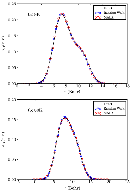
The total nuclear probability density evaluated as histograms from the Metropolis random walk and MALA simulations are compared to the grid-based result from Alexander et al. Alexander2001 in Fig. 1. The distributions converged to the exact probability density after 2×1072superscript1072\times 10^{7} steps with 8 beads at both temperatures of 8K and 30K.
Refer to caption
Figure 1: The estimated nuclear probability densities of Alexander’s model Alexander2001 at (a) 8K and (b) 30K. For path integral Monte Carlo simulations, densities were obtained by histograms with 50 bins. The discretization number of 8 was enough to converge to the exact probability densitiies.

III.2 Model of a chromophore heterodimer with displaced harmonic oscillators

To test the proposed method, a system of two chromophores in a photosynthetic complex was modeled using displaced harmonic oscillator model. In this model, the ground and excited electronic states of the monomer are modeled as harmonic oscillators with different displacement, but the same harmonic constant May2004 . The thermal reduced density matrix was calculated within the single exciton manifold. The Hamiltonian for this model is then given as follows:

Vg(x1,x2)subscript𝑉𝑔subscript𝑥1subscript𝑥2\displaystyle V_{g}(x_{1},x_{2}) =12(k1x12+k2x22),absent12subscript𝑘1superscriptsubscript𝑥12subscript𝑘2superscriptsubscript𝑥22\displaystyle=\frac{1}{2}(k_{1}x_{1}^{2}+k_{2}x_{2}^{2}),
Ve(x1,x2)subscript𝑉𝑒subscript𝑥1subscript𝑥2\displaystyle V_{e}(x_{1},x_{2}) =(12k1{(x1d1)2x12}+ε1JJ12k2{(x2d2)2x22+ε2}),absent12subscript𝑘1superscriptsubscript𝑥1subscript𝑑12superscriptsubscript𝑥12subscript𝜀1𝐽𝐽12subscript𝑘2superscriptsubscript𝑥2subscript𝑑22superscriptsubscript𝑥22subscript𝜀2\displaystyle=\left(\begin{array}[]{cc}\frac{1}{2}k_{1}\{(x_{1}-d_{1})^{2}-x_{1}^{2}\}+\varepsilon_{1}&J\\ J&\frac{1}{2}k_{2}\{(x_{2}-d_{2})^{2}-x_{2}^{2}+\varepsilon_{2}\}\end{array}\right), (21)
\displaystyle\mathcal{M} =(m100m2).absentsubscript𝑚100subscript𝑚2\displaystyle=\left(\begin{array}[]{cc}m_{1}&0\\ 0&m_{2}\end{array}\right). (24)
Parameter Value
k1subscript𝑘1k_{1} 2.227817×1032.227817superscript1032.227817\times 10^{-3}
k2subscript𝑘2k_{2} 2.227817×1032.227817superscript1032.227817\times 10^{-3}
d1subscript𝑑1d_{1} 3.000003.000003.00000
d2subscript𝑑2d_{2} 2.000002.000002.00000
ε1subscript𝜀1\varepsilon_{1} 8.064745×1028.064745superscript1028.064745\times 10^{-2}
ε2subscript𝜀2\varepsilon_{2} 7.976238×1027.976238superscript1027.976238\times 10^{-2}
J𝐽J 4.738588×1044.738588superscript104-4.738588\times 10^{-4}
m1subscript𝑚1m_{1} 3.418218×1063.418218superscript1063.418218\times 10^{6}
m2subscript𝑚2m_{2} 3.418218×1063.418218superscript1063.418218\times 10^{6}
Table 2: Summary of the parameters for the displaced harmonic oscillator model used in Sec. III.2. All values are given in atomic units.

Some of the parameters were set according to our molecular dynamics/quantum chemistry calculation of the FMO complex Shim2012 . The parameter values are listed in table 2.

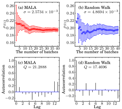
The model system was simulated at seven different temperatures ranging from 30K to 300K with a number of beads (discretization number) of 4, 8, 16, 32 and 64. The number of timesteps propagated in each simulation was 4×1074superscript1074\times 10^{7}. The value of each timestep was tuned so that the acceptance ratio of the MALA run is close to 0.574, and 0.234 for the Metropolis random walk as maintaining these acceptance ratio is known to provide most efficient sampling Pillai2011 . We used non-overlapping batch means Flegal2010 with a batch size of 106superscript10610^{6} to estimate the standard error of the correlated samples. The batch size was adjusted so that the null hypothesis of uncorrelated batches was not rejected by using Ljung-Box test Ljung1978 at a significance level of 5%percent55\%.

Refer to caption
Figure 2: Estimates of (1,2) matrix elements of the thermal reduced density matrix evaluated using MALA and Metropolis random walk at 77K with 64 beads. MALA estimate has a smaller confidence interval thus a more accurate estimate than that of the Metropolis random walk. The error bar indicates the 95% confidence interval evaluated with the batch means. The 0.950.950.95 quantile of the χ2superscript𝜒2\chi^{2} distribution with 13 degrees of freedom is 22.362 and both Ljung-Box statistics (Q𝑄Q) are smaller. Thus, the uncorrelation hypothesis is not rejected in both cases at the 5% significance level.

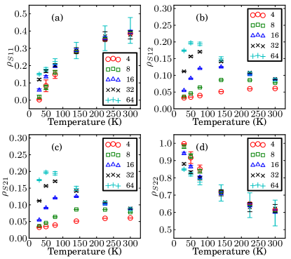
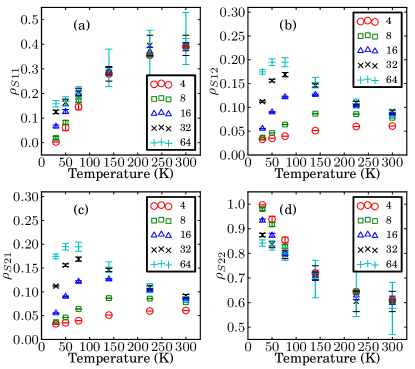
As shown in Fig. 2, the standard error of the simulation decreases modestly as the number of Monte Carlo steps increases. Fig. 3 shows the temperature dependence of the estimates of reduced density matrix elements as a function of various discretization numbers using MALA. Although the Metropolis random walk simulation gives a smaller confidence interval for the 4 bead case, MALA provides better estimates as the dimension of the sample space increases. The Metropolis random walk result is given in Fig. 4. While the population of the low energy site decreases as the temperature increases, the quantum coherence does not monotonically decrease. We believe that this pheonomenon is an artifact of an insufficient discretization number at low temperatures. As can be seen in Fig. 3, 64 or more beads are needed for the coherence to converge at 77K, while 16 beads are enough at 300K with acceptable accuracy. This is a well known limition of imaginary time path integral Monte Carlo simulations. Figure 5 shows the probability density function of the phonon coordinate at 77K and 300K. The population difference in the reduced density matrix is reflected to the difference in the probability mass of the two diabatic potential energy minimum at (3,0)30(3,0) and (0,2).02(0,2).

Refer to caption
Figure 3: Estimates of matrix elements of the thermal reduced density matrix evaluated at 30K, 50K, 77K, 140K, 225K and 300K with different discretization numbers of 4, 8 and 16 using MALA. (a) is the (1,1) element, (b), (c) and (d) are (1,2), (2,1) and (2,2) elements, respectively. The error bar indicates the 95% confidence interval evaluated with the batch means.
Refer to caption
Figure 4: Estimates of matrix elements of the thermal reduced density matrix evaluated at 30K, 50K, 77K, 140K, 225K and 300K with different discretization numbers of 4, 8 and 16 using random walk Metropolis. (a) is the (1,1) element, (b), (c) and (d) are (1,2), (2,1) and (2,2) elements, respectively. The error bar indicates the 95% confidence interval evaluated with the batch means.
Refer to caption
Figure 5: The phonon probability density function evaluated at (a) 77K and (b) 300K with 16 beads using MALA. At the lower temperature, the contribution of the exciton with lower energy at (0,2)02(0,2) becomes larger. Therefore, the population differenece becomes more distinct, as can be seen in the temperature dependence of the exciton population in Fig. 3.

IV Conclusion

We explore a method for obtaining the thermal reduced density matrix of an exciton system coupled to an arbitrary phonon bath for path integral Monte Carlo simulation. Note that our scheme is closely related to the path integral Monte Carlo simulation for nonadiabatic systems for vibrational coherence Schwieters1999 ; Alexander2001 ; Schmidt2007 . Although the phonon state can be obtained as a byproduct, we mainly focused on the evaluation of the reduced density matrix of the excitonic system to explore the asymptotic behavior of the populations and coherences in this paper. In addition, we implemented an importance sampling scheme for better spatial scaling and sampling efficiency. Although the path integral Monte Carlo cannot evaluate the real time evolution of density matrices, the method gives the exact asymptotic values with all quantum effects from both the system and bath environments if a sufficient number of beads are used. We believe that in some of the cases where the bath has a nontrivial coupling to the system, or the non-Markovianity of the bath manifests very strongly, treating the environment around the system of interest as a set of harmonic oscillators is not sufficient. If this is the case, the system should be studied in its entirety. We are trying to develop a real time propagation scheme to treat the system exactly, and the bath semiclassically. The method studied in this paper offers a foundation for it by providing the correct asymptotic behaviors.

Acknowledgements.
S.S. thanks the Samsung Scholarship for financial support. This work was supported by the Defense Advanced Research Project Agency Award No. N66001-10-4060 and by the Center of Excitonics, and Energy Frontier Research Center funded by the U.S. Department of Energy, Office of Science, and Office of Basic Energy Sciences under Award No. DE-SC0001088. A.A.-G. also acknowledges generous support from the Alfred P. Sloan and the Camille and Henry Dreyfus foundations.

References

  • (1) G. S. Engel, T. R. Calhoun, E. L. Read, T.-K. Ahn, T. Mancal, Y.-C. Cheng, R. E. Blankenship, and G. R. Fleming, Nature. 446, 782 (2007).
  • (2) G. Panitchayangkoon, D. Hayes, K. A. Fransted, J. R. Caram, E. Harel, J. Wen, R. E. Blankenship, and G. S. Engel, Proc. Natl Acad. Sci. USA. 107, 12766 (2010).
  • (3) G. S. Schlau-Cohen, A. Ishizaki, T. R. Calhoun, N. S. Ginsberg, M. Ballottari, R. Bassi, and G. R. Fleming, Nat. Chem. advance online publication. (2012).
  • (4) C. Y. Wong, R. M. Alvey, D. B. Turner, K. E. Wilk, D. A. Bryant, P. M. G. Curmi, R. J. Silbey, and G. D. Scholes, Nat. Chem. advance online publication. (2012).
  • (5) E. Collini, C. Y. Wong, K. E. Wilk, P. M. G. Curmi, P. Brumer, and G. D. Scholes, Nature. 463, 644 (2010).
  • (6) A. Kolli, E. J. O’Reilly, G. D. Scholes, and A. Olaya-Castro, The fundamental role of localised vibrations in excitation dynamics in photosynthetic light-harvesting systems, arXiv:1203.5056v1, 2012.
  • (7) T. Föster, Ann. Phys. 437, 55 (1948).
  • (8) V. May and O. Kühn, Charge and Energy Transfer Dynamics in Molecular Systems, Wiley-VCH Verlag, Weinheim, 2004.
  • (9) A. G. Redfield, IBM J. Res. Dev. 1, 19 (1957).
  • (10) H. Haken and P. Reineker, Z. Phys. 249, 253 (1972).
  • (11) H. Haken and G. Strobl, Z. Phys. 262, 135 (1973).
  • (12) A. Ishizaki and Y. Tanimura, J. Phys. Soc. Jpn 74, 3131 (2005).
  • (13) A. Ishizaki and G. R. Fleming, J. Chem. Phys. 130, 234111 (2009).
  • (14) A. Ishizaki and G. R. Fleming, Proc. Natl Acad. Sci. USA. 106, 17255 (2009).
  • (15) M. Topaler and N. Makri, J. Chem. Phys. 97, 9001 (1992).
  • (16) N. Makri, Chem. Phys. Lett. 193, 435 (1992).
  • (17) J. Zhu, S. Kais, P. Rebentrost, and A. Aspuru-Guzik, J. Phys. Chem. B. 115, 1531 (2011).
  • (18) R. Feynman and F. Vernon, Ann. Phys. 24, 118 (1963).
  • (19) S. Shim, P. Rebentrost, S. Valleau, and A. Aspuru-Guzik, Biophys. J. 102, 649 (2012).
  • (20) C. Olbrich and U. Kleinekathöfer, J. Phys. Chem. B. 114, 12427 (2010).
  • (21) C. Olbrich, J. Strümpfer, K. Schulten, and U. Kleinekathöfer, J. Phys. Chem. B 115, 758 (2011).
  • (22) D. Thirumalai, E. J. Bruskin, and B. J. Berne, J. Chem. Phys. 79, 5063 (1983).
  • (23) K. Allinger, B. Carmeli, and D. Chandler, J. Chem. Phys. 84, 1724 (1986).
  • (24) E. C. Behrman, G. a. Jongeward, and P. G. Wolynes, J. Chem. Phys. 83, 668 (1985).
  • (25) J. Cao and B. J. Berne, J. Chem. Phys. 99, 2902 (1993).
  • (26) J. M. Moix, Y. Zhao, and J. Cao, Phys. Rev. B 85, 115412 (2012).
  • (27) C. P. Robert and G. Casella, Monte Carlo statistical methods., Springer Verlag, New York, 2004.
  • (28) N. S. Pillai, A. M. Stuart, and A. H. Thiery, Optimal Scaling and Diffusion Limits for the Langevin Algorithm in High Dimensions, arXiv:1103.0542v2, 2011.
  • (29) A. Aspuru-Guzik and W. A. Lester Jr., Quantum Monte Carlo methods for the solution of the Schrödinger equation for molecular systems, in Special Volume, Computational Chemistry, edited by C. L. Bris, volume 10 of Handbook of Numerical Analysis, pp. 485 – 535, Elsevier, 2003.
  • (30) M. H. Alexander, Chem. Phys. Lett. 347, 436 (2001).
  • (31) J. M. Flegal and G. L. Jones, Ann. Stat. 38, 1034 (2010).
  • (32) G. M. Ljung and G. E. P. Box, Biometrika. 65, 297 (1978).
  • (33) C. D. Schwieters and G. a. Voth, J. Chem. Phys. 111, 2869 (1999).
  • (34) J. R. Schmidt and J. C. Tully, J. Chem. Phys. 127, 094103 (2007).