Critical behavior of the SIS epidemic model with time-dependent infection rate

Abstract

In this work we study a modified Susceptible-Infected-Susceptible (SIS) model in which the infection rate $\lambda$ decays exponentially with the number of reinfections $n$, saturating after $n=l$. We find a critical decaying rate $\epsilon_{c}(l)$ above which a finite fraction of the population becomes permanently infected. From the mean-field solution and computer simulations on hypercubic lattices we find evidences that the upper critical dimension is $6$ like in the SIR model, which can be mapped in ordinary percolation.

Keywords: Stochastic Processes, Epidemic Models, Population Dynamics, Monte Carlo Simulation

1 Introduction

Epidemic models have long been studied in the physics community both to infer patterns and to develop policies to stop and prevent epidemics on natural environments [1, 2, 3, 4] and as a playground to test theoretical ideas [5, 6, 7, 8]. In the simplest models, individuals can be either susceptible or infected and, in the latter case, can infect others with a given infection rate. If, after some time, the infected individual is susceptible to reinfection the model is known susceptible-infected-susceptible (SIS). If, otherwise, infected individuals become immune it is called susceptible-infected-recovered (SIR) model. Despite the simplicity of these models, they have succesfully modelled a varied class of diseases, like dengue [9, 10, 11], HIV [12, 13] and influenza A (H1N1) [1, 2, 14, 15].

A fundamental question in the analysis of epidemic models is whether a disease will spread through a finite fraction of the population or will it only affect a small fraction of the individuals. Also of great importance is the development of efficient immunization strategies, both answers depending fundamentally on the underlying topology of interconnections between individuals of the population [16].

Although one could create a variety of infection dynamics and network structures, an exact mapping of epidemic models onto reaction-diffusion models [6] and subsequent development of operator algebras and field-theories [17, 18, 19] show that a small number of universality classes might exist, linking different models to the same quantitative behavior around the onset of epidemic state [18, 20]. Scaling analysis also reveal that an upper critical dimension might exist for each process, above which dimensional effects are irrelevant and critical exponents and amplitude ratios are the same as in the mean-field approximation (which mimics infinite-dimensional systems, as the number of individuals $N\to\infty$).

Effects of network topology might also affect the properties of epidemic models: while on networks with randomly connected agents there is a finite threshold separating epidemic from non-epidemic states, networks with large connectivity fluctuations, such as scale-free networks, lack epidemic thresholds on both SIS and SIR models [7, 21, 22, 23, 24, 25, 26].

In this work we study a modified version of the SIS model. In particular, we consider a decaying infection rate $\lambda$, i.e., each individual $j$ that recovers from the infected state in a certain time step $t$ decreases his probability to becomes infected again in the next time step $t+1$ in the form $\lambda_{j}(t+1)=\epsilon\,\lambda_{j}(t)$, where $\epsilon$ is a parameter of the model. In addition, the decrease of the infection rate occurs only a limited number $l$ of times. This type of infectivity has been known to occur both in plants [27] and in the Simian Immunodeficiency Virus infection [28]. We study the model on regular lattices and in the mean-field regime, and considering the above-mentioned modification, our results suggest that the system undergoes a phase transition at critical values $\epsilon_{c}(l)$ separating a phase where the disease reaches a finite fraction of the population ($\epsilon>\epsilon_{c}$) from a phase where the disease does not spread out ($\epsilon\leq\epsilon_{c}$). We also find that the upper critical dimension is $6$, as in the SIR model [6, 7].

2 Model and Mean-Field Approach

The population is classified into two classes: Susceptible (S) and Infected (I). The transitions between the states $S$ and $I$ occur according to the following automata rules:

• If individual $j$ is Infected at time $t$, it is Susceptible at time $t+1$ with probability $\alpha$;

• If, otherwise, individual $j$ is Susceptible at time $t$, then with probability $\lambda$ it becomes Infected at time $t+1$ if it is in contact with an Infected individual at the same time;

• Each individual $j$ starts with $\lambda(j,t=0)=\lambda_{0}$, but $\lambda$ depends on how many times the individual was infected before, i.e., if an individual $j$ performed the transition $I\to S$ in a certain time step $t$, in the following time step $t+1$ the infection rate $\lambda$ will be updated in the following form

  $$\lambda(j,t+1)=\epsilon\,\lambda(j,t)~{},$$

  where $\epsilon$ is a parameter less than $1$ that controls the decaying of the infection rate.

• In addition, this decay in the infection rate occurs only a maximum number $l$ of times, i.e., each individual has a limited capacity to decrease his probability of reinfection.

This dynamics can be relevant to describe diseases such as flu, for which our chance to be reinfected decreases with age. The above rules define a mean-field-like system because all individuals interact with all others. Thus, an analytic approach can be developed, based on the standard ordinary differential equations for SIS models. We can define $S_{k}$ as the density of Suceptible individuals that have recovered $k$ times from the disease, with $\lambda_{k}=\epsilon^{k}\lambda_{0}$ being the corresponding infection rate of these individuals. Considering that after some time steps (nothing to do with the steady state of the system) all individuals will be in two states, $I$ or $S_{l}$, we can see that the only important equation in the evolution of the system is the equation for $S_{l}$, i.e.,

Figure 1: Density of Susceptible individuals $S(t)$ (left side, from top to bottom: $\epsilon=0.80,0.85,...,1.00$) and density of Infected individuals $I(t)$ (right side, from top to bottom: $\epsilon=1.00,0.98,...,0.80$) as functions of time $t$ for a population of size $N=10^{5}$, limiting parameter $l=5$ and typical values of $\epsilon$. Data are averaged over $200$ realizations. In this case, for $\epsilon<\sim 0.87$ the disease does not spread in the system. The parameters are: $\alpha=0.05$ and $\lambda_{0}=0.1$.

$$\frac{dS_{l}}{dt}=\alpha I-\lambda_{l}S_{l}I~{}.$$ (1)

Taking into account that in the steady state, i.e., for $t\to\infty$, we have that $S_{l}=S_{{\rm steady}}$ and $dS_{l}/dt=dS_{{\rm steady}}/dt=0$, Eq. (1) give us

$$I_{{\rm steady}}\left(\alpha-\epsilon^{l}\lambda_{0}S_{{\rm steady}}\right)=0~{},$$ (2)

where we have used the notations $S_{{\rm steady}}$ and $I_{{\rm steady}}$ to represent the stationary density of Susceptible and Infected individuals, respectively, i.e., $S_{{\rm steady}}=S(t\to\infty)$ and $I_{{\rm steady}}=I(t\to\infty)$. There are two solutions of Eq. (2): $I_{{\rm steady}}=0$ and $I_{{\rm steady}}=1-(\alpha/\lambda_{0})\epsilon^{-l}$, where we have used the relation $S+I=1$. Notice that the nontrivial solution for $I_{{\rm steady}}$ may vanishes for critical values of $\epsilon$ given by

$$\epsilon_{c}=\left(\frac{\alpha}{\lambda_{0}}\right)^{1/l}~{}.$$ (3)

Using this result, we can rewrite the expression for $I_{{\rm steady}}$ as

$$I_{{\rm steady}}=1-\left(\frac{\epsilon_{c}}{\epsilon}\right)^{l}~{}.$$ (4)

Figure 2: Stationary density of Susceptible individuals $S_{{\rm steady}}$ for $l=5$ and some values of $\epsilon$ in the log-log scale. The straight line has slope $-5$ (left side). For the stationary density of Infected individuals $I_{{\rm steady}}$ we do not have a power-law dependency on the parameter $\epsilon$, as predicted analytically in Eq. (4). Thus we plot here $I^{*}_{{\rm steady}}=1-I_{{\rm steady}}$, and the slope of the straight line is $-5$ (right side). The parameters are: $N=10^{5}$, $\alpha=0.05$ and $\lambda_{0}=0.1$. Each point is averaged over 200 realizations.

In other words, we have a Disease-free phase, where the disease disappears of the system, for $\epsilon\leq\epsilon_{c}(l)$, with the critical values $\epsilon_{c}(l)$ given by Eq. (3). On the other hand, for $\epsilon>\epsilon_{c}(l)$ we have an Epidemic phase, where the disease survives and reaches a finite fraction of the population. Considering again the relation $S+I=1$, we can obtain a power-law relation between the stationary density of Susceptible individuals and the parameters of the system,

$$S_{{\rm steady}}=\left(\frac{\alpha}{\lambda_{0}}\right)\epsilon^{-l}~{}.$$ (5)

Figure 3: Density of Susceptible individuals $S(t)$ (left side, from top to bottom: $\epsilon=0.90,0.92,...,1.00$) and density of Infected individuals $I(t)$ (right side, from top to bottom: $\epsilon=1.00,0.98,...,0.90$) as functions of time $t$ for $N=10^{5}$ and limiting parameter $l=10$. Data are averaged over $200$ realizations. Notice that in this case the disease disappears of the system for $\epsilon<\sim 0.93$. The parameters are: $\alpha=0.05$ and $\lambda_{0}=0.1$.

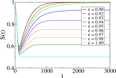
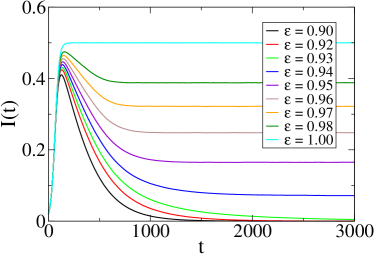
After the development of the analytical solution of the problem, we can confront it with Monte Carlo simulations. We simulated populations of size $N=10^{5}$, with probabilities $\alpha=0.05$ and $\lambda_{0}=0.1$ and different values of $\epsilon$ and $l$. We considered that $2\%$ of the individuals are initially Infected in the population, and all results were averaged over $200$ realizations. Following the rules presented in the beggining of this section, the algorithm to simulate the problem is as follows: (i) at each time step, each Infected individual $j$ returns to the Susceptible state with probability $\alpha$; (ii) at the same time, each Susceptible individual $j$ becomes Infected with probability $\lambda_{j}$ if a randomly choosen node is Infected. After each transition $I\to S$, the infection rate decreases in the form $\lambda_{j}\to\epsilon\;\lambda_{j}$.

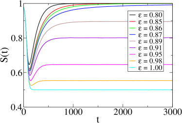
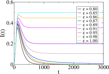
In Fig. 1 we exhibit results for the density of Susceptible individuals $S(t)$ and the density of Infected individuals $I(t)$ as functions of the simulation time $t$ for $l=5$ and typical values of $\epsilon$. We can observe that the system reaches steady states for all values of $\epsilon$, and that for $\epsilon<\sim 0.87$ the disease disappears of the system, i.e., we have $I=0$ for large $t$. Considering the mean-field calculations derived in the beggining of this section, the analytical prediction of Eq. (3) for this critical value is $\epsilon_{c}(l=5)\cong 0.87055$, in excellent agreement with the numerical result.

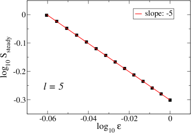
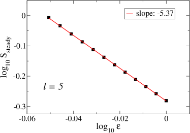
We can analyze how the stationary values $S_{{\rm steady}}=S(t\to\infty)$ depend on the parameter $\epsilon$. For this purpose, we have considered time averages of the density of susceptible individuals (after the system reach the steady states), and in addition these values were averaged over $200$ realizations of the system, for each value of $\epsilon$. We can observe the power-law behavior (see Fig. 2, left side)

$$S_{{\rm steady}}\sim\epsilon^{-\nu}~{},$$ (6)

Figure 4: Stationary density of Susceptible individuals $S_{{\rm steady}}$ for $l=10$ and some values of $\epsilon$ in the log-log scale. The straight line has slope $-10$. The parameters are $\alpha=0.05$ and $\lambda_{0}=0.1$. Each point is averaged over 200 realizations.

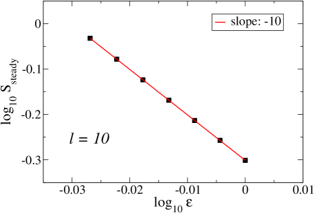
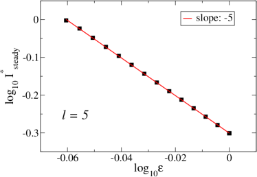
with $\nu=5$ in this case ($l=5$). Notice that this result is in agreement with the analytical prediction, Eq. (5). On the other hand, for the stationary values $I_{{\rm steady}}=I(t\to\infty)$ we do not have a power-law behavior, as predicted analytically in Eq. (4). However, we can analyze the behavior of $I^{*}_{{\rm steady}}=1-I_{{\rm steady}}$, for which Eq. (4) give us

$$I^{*}_{{\rm steady}}=\left(\frac{\epsilon_{c}}{\epsilon}\right)^{l}~{},$$ (7)

or in other words, $I^{*}_{{\rm steady}}\sim\epsilon^{-l}$, the same behavior observed for $S_{{\rm steady}}$ [see Eq. (5)]. Thus, in Fig. 2 (right side), we exhibit the simulation data for $I^{*}_{{\rm steady}}$ versus $\epsilon$ for $l=5$. Fitting data, we obtained $I^{*}_{{\rm steady}}\sim\epsilon^{-5}$ , in agreement with the analytical result, Eq. (7).

In Fig. 3 we show results for $l=10$ and different values of $\epsilon$. Again, the system reaches steady states for all $\epsilon$, but the disease spreads in the system only for $\epsilon>\sim 0.93$. Observe that this critical value $\epsilon_{c}(l=10)$ is greater than the value $\epsilon_{c}(l=5)\sim 0.87$, as expected, due to the greater capacity of the individuals to decrease their reinfection rates. The analytical result of Eq. (3) for this critical value is $\epsilon_{c}(l=10)\cong 0.93303$, again in excellent agreement with the numerical result.

Figure 5: Stationary density of Susceptible individuals $S_{{\rm steady}}$ as a function of $\epsilon$ for different values of $l$. The straight lines are fittings, which give us $S_{{\rm steady}}\sim\epsilon^{-\nu(l)}$, with $\nu(l)=l$ (left side). It is also shown the exponent $\nu$ as a function of $l$ (right side). The squares were estimated from the fittings, whereas the line is the analytical prediction, Eq. (5). The parameters in both figures are $\alpha=0.05$ and $\lambda_{0}=0.1$.

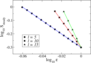
Considering the stationary values $S_{{\rm steady}}$ for different values of $\epsilon$, we can also observe a power-law behavior $S_{{\rm steady}}\sim\epsilon^{-\nu}$ (see Fig. 4), but now with a different exponent, $\nu=10$. In other words, we have the general form

$$S_{{\rm steady}}\sim\epsilon^{-\nu(l)}~{},$$ (8)

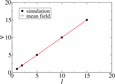
with $\nu(l)=l$, which is supported by numerical results for other values of $l$ (see Fig. 5, left side). In addition, the analytical prediction of Eq. (5) give us the same behavior of the above numerical result, Eq. (8), as we can see in Fig. 5 (right side).

Figure 6: Phase diagram of the model in the plane $\epsilon$ versus $l$, separating the Disease-free and the Epidemic phases. The squares were estimated from the simulation data, whereas the full (red) line is the mean-field prediction, Eq. (3). The parameters are $\alpha=0.05$ and $\lambda_{0}=0.1$.

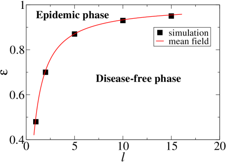
Taking into account the numerical results for $\alpha=0.05$, $\lambda_{0}=0.1$ and different values of the parameters $\epsilon$ and $l$, we show in Fig. 6 the phase diagram of the model separating the Disease-free and the Epidemic phases. The squares are the critical values $\epsilon_{c}(l)$ estimated from the simulation data, whereas the curve is the analytical prediction of Eq. (3). We can observe an excellent agreement between the analytical and the Monte Carlo results.

In the next section we will analyze how the presence of a regular topology affects the system and the mean-field results presented in this section.

3 Simulations on regular d-dimensional lattices

Figure 7: Density of Infected individuals $I(t)$ as a function of time $t$ for the model defined on a square lattice. The parameters are $l=2$ (left side, from top to bottom: $\epsilon=1.00,0.98,0.96,...,0.86$) and $l=5$ (right side, from top to bottom: $\epsilon=1.00,0.99,0.98,...,0.90$) and typical values of $\epsilon$. Data are averaged over $200$ realizations. We have used in these simulations $L=1000$, $\alpha=0.05$ and $\lambda_{0}=0.1$.

In this section we will analyze the same model presented in the last section, but now it will be defined on regular d-dimensional lattices of linear sizes $L$. The algorithm to simulate the problem is as follows: (i) at each time step, each Infected individual $j$ returns to the Susceptible state with probability $\alpha$; (ii) at the same time, each Susceptible individual $j$ becomes Infected with probability $m\,\lambda(j,t)/z$, where $m=0,1,...,z$ is the number of infected nearest neighbors of the individual $j$, $z$ is the coordination number of the d-dimensional lattice ($z=2d$) and $\lambda(j,t)$ is the infection probability of the individual $j$ at a certain time step $t$. After each transition $I\to S$, the infection rate of an individual decreases in the form $\lambda\to\epsilon\;\lambda$.

Initially, we will consider a square lattice. Thus, we have $N=L^{2}$ individuals, and each individual interact with four neighbors ($z=4$). We have observed that the results do not depend strongly on the lattice size. Thus, we simulated populations of size up to $N=10^{6}$ individuals, i.e., for linear sizes up to $L=1000$, with probabilities $\alpha=0.05$ and $\lambda_{0}=0.1$ and different values of $\epsilon$ and $l$. We have considered that $2\%$ of the individuals are initially Infected in the population. All results were averaged over $200$ realizations.

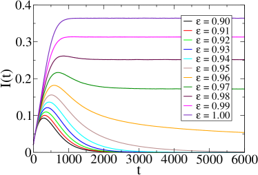
In Fig. 7 we show results for the density of Infected individuals as a function of time for $l=2$ (left side) and $l=5$ (right side). We can see that, at least qualitatively, the results are the same as in the mean-field limit. However, the critical values $\epsilon_{c}(l)$ are different. As examples, we can see in Fig. 7 that we have $\epsilon_{c}(l=2)\sim 0.88$ and $\epsilon_{c}(l=5)\sim 0.95$, whereas we have for the mean-field case $\epsilon_{c}(l=2)\sim 0.71$ and $\epsilon_{c}(l=5)\sim 0.87$. In other words, the difference bewteen the two analyses increases for increasing values of $l$. This is a consequence of the presence of a topology (neighborhood) in the model.

Figure 8: Stationary density of Susceptible individuals $S_{{\rm steady}}$ as a function of $\epsilon$ in the log-log scale for the model defined on a square lattice. The parameters are $l=2$ (left side) and $l=5$ (right side). Notice that the pure power-law behavior of Eq. (5) is not observed in the 2D case. However, there are two distinct power-law behaviors (full and dashed lines). We have used in these simulations $L=1000$, $\alpha=0.05$ and $\lambda_{0}=0.1$. Each point is averaged over 200 realizations.

Figure 9: Stationary density of Susceptible individuals $S_{{\rm steady}}$ as a function of $\epsilon$ in the log-log scale for the model defined on a simple cubic lattice. The parameters are $l=2$ (left side) and $l=5$ (right side). Notice that the pure power-law behavior of Eq. (5) is not observed in the 3D case. However, there are two distinct power-law behaviors (full and dashed lines). We have used in these simulations $L=50$, $\alpha=0.05$ and $\lambda_{0}=0.1$. Each point is averaged over 200 realizations.

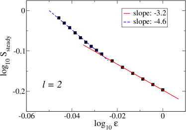
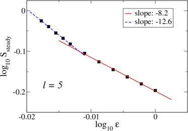
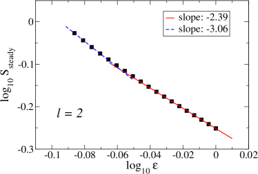
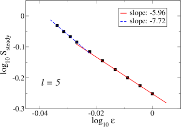
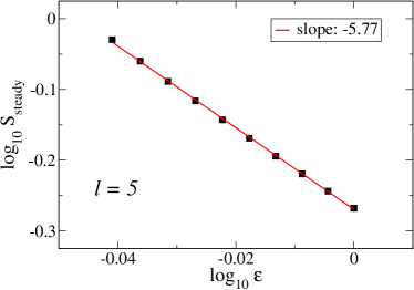
Following the procedure of the previous section, we can analyze the behavior of the stationary density of Susceptible individuals $S_{{\rm steady}}$ as a function of $\epsilon$, for different values of $l$. We show in Fig. 8 results for $l=2$ (left side) and $l=5$ (right side). We can observe deviations of the single power-law behavior given by Eq. (5). The $S_{{\rm steady}}$ values follow power laws with two different exponents: one for values of $\epsilon$ near the critical point (bigger slope, dashed lines in Fig. 8), and another to intermediary and large values of $\epsilon$, with a smaller slope (full lines in Fig. 8). The same behavior was observed for the system defined on a simple cubic lattice ($z=6$), as we can see in Fig. 9. This may be viewed as a consequence of a small number of neighbors. In fact, if we consider higher-dimensional lattices we recover a similar mean-field behavior, i.e., a power-law dependency of the $S_{{\rm steady}}$ on the parameter $\epsilon$ (see Fig. 10). Considering for example $l=5$, the numerical results give us $S_{{\rm steady}}(l=5)\sim\epsilon^{-5.77}$, $S_{{\rm steady}}(l=5)\sim\epsilon^{-5.55}$, $S_{{\rm steady}}(l=5)\sim\epsilon^{-5.37}$ and $S_{{\rm steady}}(l=5)\sim\epsilon^{-5.34}$ for $d=4$, $d=5$, $d=6$ and $d=7$, respectively. In other words, these results suggest that for $d\geq 6$ the system presents a similar behavior observed in the mean-field level, with a difference less than $7\%$ to the mean-field exponent [see Eq. (5)]. A similar behavior was also observed for other values of the parameter $l$ as $l=2$ and $l=10$.

Figure 10: Stationary density of Susceptible individuals $S_{{\rm steady}}$ as a function of $\epsilon$ in the log-log scale for the model defined on hypercubic lattices with dimensions $d=4$ (left side) and $d=6$ (right side). Notice that the pure power-law behavior of Eq. (5) is observed for $d\geq 4$, and that for $d=6$ we have essentially the same behavior as in the mean-field case, i.e., we have $S_{{\rm steady}}\sim\epsilon^{-l}$. The parameters used in the simulations are $\alpha=0.05$, $\lambda_{0}=0.1$, and the lattice sizes considered were $L=20$ (for $d=4$) and $L=8$ (for $d=6$). Each point is averaged over 200 realizations.

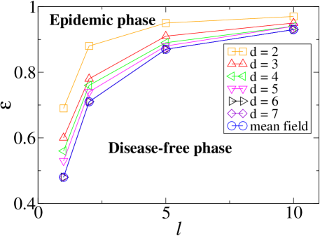
This picture becomes more clear if we estimate the critical values $\epsilon_{c}(l)$ for different dimensions $d$. In Fig. 11 we exhibit the phase diagram of the model for some values of $d$. Notice that the Epidemic phase increases for increasing values of the dimensionality $d$. This is a consequence of the increasing number of neighbors (or the coordination number $z$) on higher-dimensional lattices: it is easier to infect an individual that has more neighbors. It can be also observed in Fig. 11 that the critical values of $\epsilon_{c}(l)$ for $d=6$, $d=7$ and for the mean-field case are indistinguishable, which reinforces that the upper critical dimension of the model is $d=6$, as in the SIR model [6, 7]. This is due to the frozen state of the individuals with very low infectivity that results from multiple reinfections.

Figure 11: Comparative phase diagram of the model in the plane $\epsilon$ versus $l$ for different dimensionalities $d$. The symbols were estimated from the simulations. Notice that the Epidemic phase increases for increasing values of $d$, and that the critical values $\epsilon_{c}(l)$ for $d\geq 6$ and for the mean-field approach are the same. The parameters are $\alpha=0.05$ and $\lambda_{0}=0.1$.

4 Conclusions

In this work we studied a modified Susceptible-Infected-Susceptible (SIS) model in which we have considered that each individual in the population that recovered from the disease decreases his probability of reinfection. This decrease occurs a maximum number $l$ of times for each individual. This dynamics can be relevant to describe diseases such as flu, for which our chance to be reinfected decreases with age.

Firstly, we have analyzed the problem in the mean-field limit. In this case, every individual interact with all others, and we studied the problem with numerical simulations and analytical calculations. Considering the initial infection rate $\lambda_{0}$ (for the transition $S\to I$) and the recovering rate $\alpha$ (for the transition $I\to S$), we have found a power-law dependency between the stationary density of susceptible individuals $S_{{\rm steady}}$ and the parameter $\epsilon$ that controls the decaying of the infection rate in the form $S_{{\rm steady}}=(\alpha/\lambda_{0})\epsilon^{-l}$. In addition, we showed that the system undergoes a phase transition at critical values $\epsilon_{c}(l)=(\alpha/\lambda_{0})^{1/l}$ separating a phase where the disease reaches a finite fraction of the population (for $\epsilon>\epsilon_{c}$) from a phase where the disease does not spread out (for $\epsilon\leq\epsilon_{c}$). All results were confirmed by Monte Carlo simulations.

Considering $d$-dimensional regular lattices, we have studied the model only with numerical simulations. The evolution of the density of Susceptible and Infected individuals is qualitatively similar to the evolution obtained in the mean-field case, but the presence of a neighborhood modify some characteristics of the model. In particular, the critical values $\epsilon_{c}(l)$ are greater than in the mean-field case for $d<6$, which implies that the epidemic phase decreases for decreasing values of $d$. However, for $d=6$ and $d=7$ we have obtained the same values of the critical points $\epsilon_{c}(l)$ as in mean-field calculations. The stationary density of susceptible individuals $S_{{\rm steady}}$ depends on the parameter $\epsilon$ in a power-law form only for $d>3$, whereas for $d=2$ and $d=3$ we have the combination of two power laws. These numerical results suggest that the upper critical dimension of the model is $d=6$ as in the SIR model. This is possibly due to the frozen state of the individuals with very low infectivity that results from multiple reinfections.

Thus, the mean-field analytical calculations describe qualitatively well the model, providing us the phenomena that are expected to be observed, i.e., it predicts the phase transition and the power-law dependency between some quantities of interest. However, it fails quantitatively, as it is common in mean-field approximations, because predicts different values of the critical points and different power-law exponents.

References

- [1] A. M. Smith, A. S. Perelson, Wiley interdisciplinary Reviews: Systems Biology and Medicine 3, 429 (2011).
- [2] P. Baccam, C. Beauchemin, C. A. Macken, F. G. Hayden, A. S. Perelson, Journal of Virology 80, 7590 (2006).
- [3] B. Gönci, V. Németh, E. Balogh, B. Szabó, A. Dénes, Z. Környei, T. Vicsek, PLoS ONE 5(12): e15571 (2010).
- [4] R. M. Anderson, R. M. May, Infectious Diseases of Humans: Dynamics and Control (Oxford University Press, 1991).
- [5] J. Marro, R. Dickman, Nonequilibrium Phase Transitions in Lattice Models (Cambridge University Press, Cambridge, 1999).
- [6] H. Hinrichsen, Advances in Physics 49, 815 (2000).
- [7] M.E.J. Newman, Phys. Rev. E 66, 016128 (2002).
- [8] N. T. J. Bailey, The Mathematical Theory of Infectious Diseases and its Applications (Hafner Press, New York, 1975).
- [9] M. Derouich, A. Boutayeb, E. H. Twizell, BioMedical Engineering 2:4 (2003).
- [10] L. Esteva, C. Vargas, J. Math. Biol. 46, 31 (2003).
- [11] N. Nuraini, E. Soewono, K. A. Sidarto, Bull. Malays. Math. Sci. Soc 30, 143 (2007).
- [12] R.M.Z. dos Santos, S. Coutinho, Phys. Rev. Lett. 87, 168102 (2001).
- [13] F. Baryarama, L. S. Luboobi, J. Y. T. Mugisha, Amer. J. Infect. Diseases 1, 55 (2005).
- [14] I. Gordo, M. G. M. Gomes, D. G. Reis, P. R. A. Campos, PLos ONE 4(3):e4876 (2009).
- [15] G. Katriel, L. Stone, PLoS Curr. 1: RRN10460 (2009).
- [16] R. Cohen, S. Havlin, D. ben-Avraham, Physical Review Letters 91, 247901 (2003).
- [17] M. Doi, J. Phys. A 9, 1479 (1976).
- [18] H. K. Janssen, Z. Phys. B 42, 151 (1981).
- [19] P. Grassberger, A. de la Torre, Ann. Phys. 122, 373 (1979).
- [20] P. Grassberger, Z. Phys. B 47, 365 (1982).
- [21] R. M. May, A. L. Lloyd, Phys. Rev. E 64, 066112 (2001).
- [22] Y. Moreno, R. Pastor-Satorras, A. Vespignani, Eur. Phys. J. B 26, 521 (2002).
- [23] R. Pastor-Satorras, A. Vespignani, Phys. Rev. E 63, 066117 (2001).
- [24] R. Pastor-Satorras, A. Vespignani, Phys. Rev. Lett. 86, 3200 (2001).
- [25] R. Parshani, S. Carmi, S. Havlin, Phys. Rev. Lett 104, 258701 (2010).
- [26] M. Boguñá, R. Pastor-Satorras, A. Vespignani, in Statistical Mechanics of Complex Networks, edited by R. Pastor-Satorras, M. Rubi and A. Díaz-Guilera (Springer Verlag, Berlib, 2003), vol. 625 of Lecture Notes in Physics.
- [27] C. A. Gilligan, S. Gubbins, S. A. Simons, Phyl. Trans. R. Soc. Lond. B 352, 353 (1997).
- [28] N. K. Vaidya, R. N. Ribeiro, C. J. Miller, A. S. Perelson, Journal of Virology 84, 4302 (2010).