Fermi edge singularity and finite frequency spectral features in a semi-infinite 1D wire
Abstract
We theoretically study a charge qubit interacting with electrons in a semi-infinite 1D wire. The system displays the physics of the Fermi edge singularity. Our results generalize known results for the Fermi-edge system to the regime where excitations induced by the qubit can resolve the spatial structure of the scattering region. We find resonant features in the qubit tunneling rate as a function of the qubit level splitting. They occur at integer multiples of . Here is the Fermi velocity of the electrons in the wire, and is the distance from the tip of the wire to the point where it interacts with the qubit. These features are due to a single coherent charge fluctuation in the electron gas, with a half-wavelength that fits into an integer number of times. As the coupling between the qubit and the wire is increased, the resonances are washed out. This is a clear signature of the increasingly violent Fermi-sea shake-up that accompanies strong coupling.
pacs:
73.40.Gk, 72.10.FkI Introduction
Systems in which a localized impurity, with an internal quantum mechanical degree of freedom, interacts with an electron gas, play an important role in many-body theory. On the one hand, they allow theorists to investigate interaction effects and many-body correlations beyond the perturbative regime. On the other hand they explain observed phenomena such as the resistance minimum (as a function of temperature) in dilute magnetic alloys, i.e. the Kondo effect.kon64 Another impurity phenomenon that has been studied extensively is the so called Fermi edge singularity.mah67 ; noz69 In its original incarnation, the effect refers to power law singularities in the soft-x-ray absorption, emission, and photoemmision spectra of metallic samples. As with the Kondo effect,pus04 the phenomenon has received renewed attention due to technological breakthroughs in nano-physics and quantum transport. The same physics that is behind the Fermi edge singularity describes for instance tunneling into and out of a small quantum dot coupled to an electron reservoir.aba04 Recent studies have focused on non-equilibrium,muz03 ; amb04 ; aba05 ; sny07 ; gut10 ; bet11 ; gut11 non-stationary,bet11b and band structuremkh11 phenomena.
In this paper, we confine our attention to the equilibrium situation but consider a setup in which the spectral function has interesting features at energies away from the singularity. The setup can be realized with current technology. The system we study consists of an electron gas interacting with a two level system (charge qubit). A concrete realization of the qubit could be an electron that may occupy the lowest two states of a double quantum dot.elz03 ; pet04 From the point of view of the electron gas, the qubit acts as a dynamic localized impurity, while from the point of view of the qubit, the electron gas acts as a dissipative environment. The qubit state-space is spanned by the vectors and . The total Hamiltonian for the system is where
| (1) |
The energy represents a gate voltage that controls the qubit level splitting and is a small tunneling amplitude between the two qubit states. Both these parameters are typically under experimental control.
The Hamiltonians describe the electron gas. The kinetic term is the same for both Hamiltonians. The finite range potentials represent the electrostatic potential produced by the qubit. This potential depends on the internal state of the qubit, so that . We will specify the system in more detail in Sec. II.
The quantity of interest in this article is the qubit tunneling rate , which is defined as follows: Consider the situation where initially the tunneling amplitude is zero, and the qubit is prepared in the state . The electron gas is allowed to equilibrate. We assume zero temperature so that it equilibrates to the Fermi-sea ground state of the Hamiltonian . At time , the tunneling amplitude is then switched on, and the state acquires a finite lifetime. Provided that this lifetime is long enough that we can still speak of well-defined qubit levels, the probability to find the qubit in the state decays exponentiallyf1
| (2) |
where is the qubit tunneling rate.
In order to formulate a quantitative criterion for when exponential decay occurs, it is useful to define an energy
| (3) |
Here are the ground state energies associated with the Fermi sea ground states of . For the system described by , the minimum energy difference between a configuration (of qubit plus Fermi gas) with the qubit in the state and one with the qubit in the state is . Due to the finite lifetime , there is an uncertainty of order in the qubit level splitting. For the energy levels associated with to remain well-defined, the minimum energy difference between a and a configuration must be much larger than this uncertainty, i.e.
| (4) |
In this regime shows exponential decay.
By applying Fermi’s Golden, one obtains
| (5) |
(See Appendix A for details). We will use this result to obtain an explicit expression for in terms of the energy and the potentials . In the original incarnation of the problem, this quantity corresponds to the photoemmision spectrum, i.e. the intensity of electrons ejected from the metal, at a fixed x-ray frequency . (See for instance Sec. IV of Ref. oth90, .)
In the language of the Fermi edge singularity, the quantity , that appears in Eq. 5 is known as the closed loop factor. (See for instance Sec. III D of Ref. oth90, .) It is known that, for much larger than the time an individual electron spends in the scattering region
| (6) |
where is the difference between the ground state energies of and and is an ultra-violet energy scale. (The branch with is implied.) The power law exponent is determined by the single particle scattering matrices associated with the fermion Hamiltonians. Explicitlyaba04 ; amb04
| (7) |
For sufficiently small , the asymptotic form of Eq. 6 gives rise to a tunneling rate
| (8) |
with the unit step function, i.e. for and for . This power law remains valid while . Here is the Fermi velocity, is the Fermi energy measured from the bottom of the conduction band, and is the band width. The length scale is the size of the scattering region. This is not necessarily the same length scale as the range of the qubit interaction potentials , which we denote . Consider for instance a qubit placed next to a semi-infinite wire. (See Fig. 1.) Here the size of the scattering region is the distance from the tip of the wire to the point closest to the qubit, which can be much larger that the range of the potential produced by the charge of the qubit. In general .
The condition comes about as follows. An energy corresponds to density fluctuations in the electron gas with wavelengths at least . The result of Eq. 8 breaks down as soon as this wavelength is short enough for these excitations to resolve the spatial structure of the scattering region. The restriction is due to the fact that Eq. 8 becomes invalid when particle or hole excitations are created in the electron gas close to the band edges.
An analytical expression for was obtained by Tanabe and Othakatan85 in the regime , where the wavelength of electrons near the Fermi level are too long to resolve the spatial structure of the scattering region, so that the potentials may be approximated as -functions. (This is referred to as the limit of contact potentials.) was found to be of the order of . In the same limit, approximate results for the finite behavior of has been obtained. As a function of , these results contain features on the scale of that are associated with the band structure of the model. For more detail the reader is referred to the review [oth90, ].
The regime of applies in a semi-conductor, where it is not uncommon for the Fermi wave-length to be large compared other length scales in the problem. However, the opposite regime, where , also has physical relevance: In a metallic sample, the Fermi wavelength is comparable to the lattice constant, while all length-scales associated with the potential are much larger. We are not aware of any work in which this regime is investigated.
In this article we study the regime where . There are two significant differences between this regime and the previously studied regime. Firstly, the ultra-violet energy is no longer of order , but rather is determined by the potential . Secondly, the rate as function of starts deviating from the power law of Eq. 8, at energies rather than at energies . The source of the deviations is no longer related to band structure, but to excitations resolving the spatial structure of the scattering region. We confine our attention to the case of an electron gas in a single chiral channel at zero-temperature. We pay particular attention to the example mentioned above of a qubit interacting with a semi-infinite wire, where . We were able to obtain exact analytical expressions for and for the closed loop factor at arbitrary times. We find that , and that depends only on the shape, not the magnitude, of , i.e. scaling leaves unchanged. We were able to compute the tunneling rate away from the threshold . We find that has resonant features at an energy scale , that reveal the nature of many-body correlations induced by the qubit. Our main results are contained in Eqs. 53, 58, 61, and 68.
Our analysis is based on the approximation of taking the limit and linearizing the electrons’ dispersion relation around the Fermi level, while still taking into account the full spatial dependence of the potentials . As pointed out by Gutman et al. (footnote 36 of Ref. gut10, ) special care must be taken when linearizing the dispersion relation in order to account for the anomalous contribution to that is related to the Schwinger anomaly.sch59 In the derivation that we present, this anomalous contribution appears quite naturally.mat65 Our results are obtained by means of bosonization,hal81 ; del98 the application of which to the Fermi edge singularity was pioneered by Schotte and Schotte.sch69 Bosonization maps the Hamiltonian of Eq. 1 onto an equivalent spin-boson model,leg87 where a spin is coupled to a bosonic bath. For the example of a semi-infinite wire interacting with a qubit at a point on the wire that is a distance from the tip of the wire, the bosonic bath spectrum has non-trivial structure. This in turn is what leads to the non-trivial finite behavior of the tunneling rate .
The rest of this article is structured as follows. In Sec. II we specialize to a Fermi gas consisting of a single chiral channel, and introduce a model to describe a semi-infinite wire interacting with a qubit at a point a distance from the tip of the wire. In Sec. III we collect the results from the theory bosonization that are required for our analysis. We also discuss Anderson’s orthogonality catastrophe from the point of view provided by bosonization. In Sec. IV we give a general and exact formula for the closed loop factor. This allows us to calculate the ultraviolet energy scale exactly. In Sec. V we apply the general results of Sec. IV to the specific system introduced in Sec. II, for which the tunneling rate has non-trivial features at finite .
II a Single chiral channel
Here we give a mathematical definition of the type of electron gas we study. Associated with the electrons in a chiral channel of length with periodic boundary conditions are creation and annihilation operators and that respectively create or annihilate a fermion in the state localized at position . They obey the usual anti-commutation relations
| (9) |
and are periodic with period . At the point in our derivation where it becomes convenient to do so, we send the system size to infinity.
The non-interacting many-fermion Hamiltonians have the same linear dispersion but different external potentials. Without loss of generality (see Appendix B for details), we can set the external potential in to zero, so that
| (10) |
while with
| (11) |
(Here we work in units where the Fermi velocity .) Associated with is the one-dimensional scattering matrix where
| (12) |
The ground state of is the Fermi-sea
| (13) |
where is the state with no particles, the operator
| (14) |
creates a fermion in a momentum eigenstate and is quantized in integer multiples of .
(a)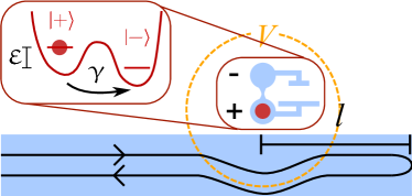 (b)
(b)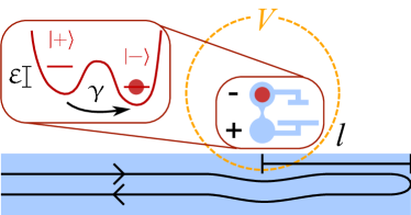
The general results we obtain will be applied to the case where the electron gas resides in a semi-infinite 1D quantum wire. In the limit of a large Fermi energy, this system is mapped onto Eqs. 1, 10, and 11 through the standard trick of “unfolding”, so that coordinates and refer to the same spatial point, but to “different sides of the road”, i.e. and create electrons at the same position but moving in opposite directions.fab95 Thus the potential is symmetric about . The system is depicted in Figure 1. As a simple model for the interaction between the qubit and the electron gas, we will take with
| (15) |
Here is the distance from the tip of the wire to the point on the wire nearest to the qubit and is the range of the potential produced by the qubit. This choice of allows us to obtain an exact analytical expression for . In the regime where we expect qualitatively similar results for any choice of that is localized to a region of length .
III Bosonization
In this section we collect together the known operator bosonization results that are required for our analysis. For a tutorial derivation, we refer the reader to Ref. del98, . Our notation closely follows Haldane’s. hal81 We use these results to write and in terms of bosonic operators. This casts the Hamiltonian into the form of a spin-boson model with a structured environment. We also calculate the overlap , where, as stated below Eq. 3, are the many body ground states of , which will be relevant when we analyze the tunneling rate in Sec. IV.
The free fermion Hamiltonian (10) together with the Fermi sea ground state is the starting point for the bosonization procedure. Associated with density fluctuations in the fermion system are operators
| (16) |
and , , that satisfy bosonic commutation relations
| (17) |
The bosonic annihilation operators annihilate the Fermi sea , i.e.
| (18) |
A central (and non-trivial) result of bosonization is that, in terms of the bosonic operators, and for fixed particle number
| (19) |
The fermion density can be expressed in terms of the bosonic operators as
| (20) |
where counts the total number of fermions and
| (21) |
The operators satisfy the commutation relations
| (22) | |||||
| (23) |
Using Eqs. 20 and 21 to express the potential in terms of the bosonic operators, and using expression 19 for , we find for
| (24) |
where
| (25) |
The Hamiltonian is diagonalized by completing the square. For this purpose we define new bosonic operators
| (26) |
that also obey the standard bosonic commutation relations. In terms of these operators the Hamiltonian reads
| (27) |
where
| (28) |
Substitution of from Eqs. 19 and 27 into the full Hamiltonian of Eq. 1 reveals that the system is described by the same Hamiltonian as the spin-boson model. (See for instance Ref. leg87, .) A quantity that plays a central role in the spin-boson model, is the bosonic environment’s spectral function which in our notation is given by
| (29) |
(Here we have implicitly taken the limit.) In the context of dissipative quantum mechanics, spectral functions for smaller than some large cut-off, play an important role. The case with is known as an Ohmic environment. We see that a potential that is peaked around , for instance , produces an Ohmic environment. When the spectral function has a more complicated form, one talks of a structured bath. A structured bath is obtained by engineering the potential . As we shall show in Sec. V, the potential of Eq. 15 produces an environment with an interesting structure.
The ground state energy of is and the ground state solves , or using the definition of in terms of ,
| (30) |
From this follows that the normalized ground state of is the coherent state
| (31) | |||||
For future reference we note that the overlap is easily calculated from Eq. 31. The details of the calculation can be found in Appendix C. The result is
| (32) |
where is the energy appearing in Eq. 6, and, consistent with Eq. 7, (cf. Eq. 12),
| (33) |
For an explicit formula for , see Eq. 58. The fact that the overlap tends to zero as is known as the orthogonality catastrophe.and67 The fact that the same ultraviolet energy appears in the closed loop factor and in the orthogonality catastrophe has previously been established (for a contact type potential) by Feldkamp and Davis fel80 , and by Tanaka and Othabetan85 .
IV Closed loop factor
In this section our goal is to calculate the closed loop factor
| (34) |
where
| (35) |
(The convenience of including the factor , with given by Eq. 28, will become apparent below.)
Having mapped the system under consideration onto a spin-boson Hamiltonian, we can simply quote the answer from the literature, namely
| (36) |
with given by Eq. 29. (See for instance Eqs. 3.35 and 3.36 of Ref. leg87, , but note that in that work refers to a different quantity than the one in Eq. 34 of the present work.) However, we prefer to give a self-contained derivation of this result. This derivation goes slightly further than simply calculating , namely, it produces a bosonic expression for the operator that is normal ordered, i.e. in which all creation operators are to the left of all annihilation operators. This expression may in future prove useful for studying non-equilibrium effects. Readers prepared to take Eq. 36 as given may wish to skip to the paragraph below Eq. 54.
The starting point of our derivation is to consider the time derivative of , i.e.
| (37) |
Since the Hamiltonian is also the momentum operator, is simply translation by a distance , so that
| (38) |
Thus we find
| (39) | |||
| (40) |
where , .
Let us now consider one of the individual factors in the ordered exponent of Eq. 40. Using Eq. 20 to relate the density operator to the bosonic operators and , we find
| (41) |
where
| (42) |
so that
| (43) |
Since operators and commute to a -number we have . Explicitly
| (44) | |||
| (45) |
We therefore find
| (46) |
When substituted back into Eq. 40, this leads to the result
| (47) |
We can rewrite this as
| (48) |
Factor is what Gutman et al.gut10 (see their footnote 36) calls the “anomalous” contribution to the closed loop factor. An expression involving the determinant of an operator acting on single particle Hilbert space often appears in the literaturemuz03 ; amb04 ; aba04 ; aba05 in connection with the closed loop factor. In Appendix E we show that this determinant is equal to the expectation value of factor .
Below we consider factors and separately. From Eq. 44 we have
| (49) |
We write factor in boson normal ordered form. This is done to facilitate the calculation of the expectation value with respect to .
| (50) | |||||
| (51) |
Explicitly evaluating the commutator in Eq. 50, we find
| (52) |
Combining this with the result in Eq. 49 for factor , we obtain
| (53) |
In the expression for , the infinite system size limit can straight-forwardly be taken to obtain
| (54) |
in agreement with Eq. 36.
The large time asymptotics of Eq. 54 can be extracted as follows. Firstly we write as
| (55) | |||||
This expression is then split up into three terms, , where
| (56) |
The integral in is straight forward and leads to where as in Eq. 33, and consistent with Eq. 7. In Appendix D we show that and hence vanishes in the large limit. Term can be written as
| (57) |
Thus, for large , we obtain where
| (58) |
This implies that is determined by the shape of but not by its overall magnitude: The transformation does not affect .
V Semi-infinite wire
We apply the results of the previous section to the case of a semi-infinite wire with given by Eq. 15 so that
| (59) |
Substitution into Eq. 54 then yields
| (60) | |||||
where . Thus in the limit of large , where
| (61) |
This last result could also have been obtained using Eq. 58. We see that , and thus also the tunneling rate , grows as for ,
Some insight into the origin of this result may be obtained by considering the result in Eq. 32 for the overlap , that displays the orthogonality catastrophe. For given by Eq. 61, . Therefore increasing mitigates the orthogonality catastrophe. The tunneling rate can be written as (cf. Eq. 74)
| (62) |
where and are the energies and many-body eigenstates of , the Hamiltonian that describes the electrons when the qubit is in state . The results of Appendix C can be extended to show that not only the ground state to ground state overlap, but every overlap where contains a finite number of particle hole excitations on top of , scales like . Thus the scaling behavior of can be understood as a consequence of the mitigation of the orthogonality catastrophe. The effect relies on the phase coherence of electrons in the section of the wire between and . Hence it is destroyed if the electron phase is randomized by impurity scattering or if there is inelastic scattering. Thus the increase in with increasing should persist until exceeds either the elastic or inelastic mean free path in the wire. Of course the result is also only valid as long as so that excitations created by the qubit do not resolve the spatial structure of the potential. Thus, the larger , the smaller the energy window in which the enhancement of due to mitigation of the orthogonality catastrophe can be observed.

The tunneling rate is calculated by expanding the third factor in Eq. 60 in a Taylor series in and Fourier transforming each term separately. Using the identities
| (63) |
for , and
| (64) |
we obtain
| (65) |
where is the result
| (66) |
The factor can be rewritten
| (67) |
Substituting this into Eq. 65 we identify the series as the Taylor expansion of the hypergeometric function , yielding one of our main results
| (68) |
As , tends to , so that indeed has the expected power law singularity for small (cf. Eq. 8) with given by Eq. 61. When becomes of the order , excitations in the wire are able to resolve the spatial structure of the potential and starts deviating from simple power law behavior. In the weak coupling limit, i.e. small , the hypergeometric function reduces to , and therefore shows oscillations with period as a function of . These oscillations can be understood as being due to the resonant creation of a single particle-hole excitation with an energy that satisfies the resonance condition . (This condition maximizes the single particle matrix element , where and refer to the single particle orbitals of the hole and the excited particle respectively.)
As shown in Figure 2, the oscillations become damped as is increased. The damping is a signature of a phenomenon known as Fermi-sea shake-up. At strong coupling (large ), rather than creating a single particle hole pair, a large number of particle hole pairs are created. This corresponds to many charge density excitations (created by the bosonic operators ) with a broad distribution of wavelengths . As a result there is no clear resonance any more, and the oscillations in are washed out.
It is also instructive to investigating the regime . Here the asymptotic behavior of the hypergeometric function is
| (69) |
If we substitute this into the expression (Eq. 68) for , assuming , we obtain
| (70) |
This is the same rate as would be obtained from a closed loop factor
| (71) |
Such a closed loop factor could also be obtained by coupling the qubit to two independent chiral channels, where the potential the qubit produces in either channel equals of Eq. 15, i.e. one of the peaks in the full potential . This means that, in the single channel semi-infinite wire, at energies , the potential experienced by right-moving electrons and the potential experienced by left-moving electrons, contribute incoherently to the rate , as if left-movers and right-movers belong to separate channels. Could this indicate that electrons reflected at the tip of the wire have lost all memory of their in-bound encounter with the qubit by the time that they again reach the qubit on their out-bound journey? Since the electrons undergo no relaxation between encounters with the qubit, the answer is “no”. Rather, what Eq. 70 indicates, is that processes in which an individual electron wave-packet with width is scattered twice, once while incident on the tip, and once after being reflected at the tip, are rare and make a vanishingly small contribution to the rate .
As stated in the introduction, corresponds to the exponential decay rate of the probability to find the qubit in state , provided that . We conclude this section by investigating when this inequality holds. For , diverges when , and the criterion for exponential decay is violated at small . From the small asymptotics , we conclude that, for , exponential decay with rate occurs when
| (72) |
When , on the other hand, no longer diverges, but rather reaches a maximum value of order at . Thus, for , exponential decay with rate occurs for all , provided that
| (73) |
The same regime for exponential decay as in Eqs. 72 and 73 was identified more rigorously by Legget et al.leg87 in the context of the spin boson Hamiltonian with an unstructured Ohmic bath (corresponding to in our system). (See their Sec. VII.B, and in particular their Eq. 7.17a. Note that the quantity that we denote is twice the quantity that they denote .) The fact that our qubit is immersed in a structured bath does not affect the result because the bath spectral function still has the same large and small asyptotics as in the case of an Ohmic bath.
VI Summary and conclusions
In this paper we studied the quantity , known in the language of the Fermi edge singularity as closed loop factor, for the case where the Hamiltonians describe electrons in a single chiral channel. We investigated the regime where is the typical length scale on which the potentials associated with vary, a regime not studied before. We investigated a system where the Fourier transform of the closed loop factor gives the tunneling rate of a two-level system (charge qubit) coupled to the electron gas. Under the assumption of linear dispersion (cf. Eq. 10) we obtained the exact expression for the closed loop factor valid for arbitrary and arbitrary times. We studied its large time asymptotics, and obtained an exact formula for the ultraviolet energy that appears in Eq. 6. Unlike in the previously studied regime where , here we find . Furthermore it turns out that is determined by the shape, but not the overall magnitude of the potentials , i.e. scaling leaves invariant.
We applied our general results to the example a semi-infinite wire. The qubit interacts with the wire at a point that is a distance from the tip of the wire. In this system we found that the tunneling rate could be enhanced without increasing either or . decreases like so that grows like . Thus the tunneling rate becomes larger the further the qubit is from the tip of the wire. This effect is due to a mitigation of the orthogonality catastrophe. It holds as long as is less than the phase-coherence length of electrons in the wire and for level splittings .
Armed with an expression for the closed loop factor that is valid also for small times, we obtain an exact expression for for the semi-infinite wire system. The finite features of probe the spatial profile of the potential at length scales (in units where ). We study how the dependence of changes as the coupling between the qubit and the electron gas grows. At weak coupling (small ), we find that the rate oscillates as a function of , and that the period is . This is due to the resonant excitation of a single particle-hole pair in the Fermi sea. The wavelength of the associated charge density fluctuation is . The resonance condition is that an integer number of half wavelengths fit into the part of the wire between the tip and the point where the qubit interacts with the wire. At strong coupling (large ) on the other hand, many particle hole excitations are created. This is known as Fermi sea shake-up. The corresponding density fluctuations have a broad distribution of wavelengths and hence there are no clear resonances. This results in the damping of the oscillations in as is increased. One of our main results (Eq. 68) is an exact formula for this damping by means of Fermi sea shake-up. The result is illustrated in Fig. 2. We also analyzed rate in the limit and saw that here the left and right moving electrons contribute to the rate as if they belong to independent channels. This happens despite the fact that each electron incident on the tip encounters the qubit twice, once before being reflected at the tip, and once afterwards, and no electron relaxation occurs between qubit encounters. The result therefore indicates that processes in which an individual electron wave-packet with width is scattered twice, once while incident on the tip and once after being reflected at the tip, make a vanishingly small contribution to the rate .
Appendix A Obtaining from Fermi’s golden rule
In this Appendix we apply Fermi’s golden rule to obtain the expression in Eq. 5 for the transition rate . The initial state for the transition is with energy . Possible final states are of the form , where is an eigenstate of and has energy . We have to sum over all eigenstates of . Thus
| (74) | |||||
Appendix B Gauging away .
In the main text we chose the potential as zero, and stated that this does not involve any loss of generality. Here we prove this claim. Suppose
| (75) |
Now define position dependent phases
| (76) |
and total phase shifts . Then define a new set of fermion operators related to by
| (77) |
The operators and obey the same anti-commutation relations as and and are also periodic with period .
Appendix C Anderson’s orthogonality catastrophe
Andersonand67 states that the overlap vanishes as a power law as the system size grows. For the present system we can calculate this overlap exactly for arbitrary potentials . Our starting point is Eq. 31 and the operator identity , provided that .
| (80) | |||||
In the large limit, we rewrite this as
| (81) |
where as in Eq. 33. The limit of the two factors marked and can be taken separately. Referring back to Eq. 58, we identify the factor marked as the energy that appears in Eqs. 6. The sum in the exponent of the factor marked is the Taylor expansion of the logarithm function and hence
| (82) |
This leads to the result
| (83) |
Appendix D Asymptotics of
In the main text, in the derivation of the asymptotic form of , we stated that in Eq. 56 vanishes like in the large limit. Here we give a proof. By Fourier transforming from to we obtain
| (84) |
The integral can be performed to obtain
| (85) |
Expanding in we find .
Appendix E Determinantal formula related to closed loop contribution
Here we show that the expectation value of the factor in Eq. 48 with respect to equals a determinant of an operator acting on single particle Hilbert space.
The proof relies on the following general result for fermionic systems. Let be a set of orthonormal single particle orbitals and let and be the associated fermionic creation and annihilation operators. Let be a subset of . Without loss of generality, we may take . Let be the many-fermion state
| (86) |
Let be the operator
| (87) |
Then , where the fermionic operator creates a particle in the orbital , where
| (88) |
is an operator acting on single particle Hilbert space. This implies that is a Slater determinant where is an matrix with entries
| (89) |
The operator projects onto the subspace spanned by the set , and hence the matrix has the same determinant as the operator , leading to the result
| (90) |
We derived this result for a state containing a finite number of particles. We postulate that a similar result holds for the state representing an infinitely deep Fermi sea.
Acknowledgements.
This research was supported by the National Research Foundation (NRF) of South Africa.References
- (1) J. Kondo, Prog. Theor. Phys. 32, 37, (1964).
- (2) G. D. Mahan, Phys. Rev. 163, 612, (1967).
- (3) P. Nozières and C. T. DeDominicis, Phys. Rev. 178, 1097, (1969).
- (4) M. Pustilnik and L. I. Glazman, J. Phys.: Condens. Matter 16, R513, (2004).
- (5) D. A.Abanin and L. S. Levitov, Phys. Rev. Lett. 93, 126802, (2004).
- (6) B. Muzykantskii, N. d’Ambrumenil, and B. Braunecker, Phys. Rev. Lett. 91, 266602, (2003).
- (7) N. d’Ambrumenil and B. Muzykantskii, arXiv:cond-mat/0405457.
- (8) D. A. Abanin and L. S. Levitov, Phys. Rev. Lett. 94, 186803, (2005).
- (9) I. Snyman and Yu. V. Nazarov, Phys. Rev. Lett. 99, 096802, (2007).
- (10) D. B. Gutman, Y. Gefen, and A. D. Mirlin, Phys. Rev. B 81, 085436, (2010).
- (11) E. Bettelheim, Y. Kaplan, and P. Wiegmann, J. Phys. A: Math. Theor. 44, 282001, (2011).
- (12) D. B. Gutman, Y. Gefen, and A. D. Mirlin, J. Phys. A: Math. Theor. 44, 165003, (2011).
- (13) E. Bettelheim, Y. Kaplan, and P. Wiegmann, Phys. Rev. Lett. 106, 166804, (2011).
- (14) V. V. Mkhitaryan and M. E. Raikh, Phys Rev. Lett. 106, 197003, (2011).
- (15) J. M. Elzerman, R. Hanson, J. S. Greidanus, L. H. Willems van Beveren, S. De Franceschi, L. M. K. Vandersypen, S. Tarucha, and L. P. Kouwenhoven, Phys. Rev. B 67, 161308R, (2003).
- (16) J. R. Petta, A. C. Johnson, C. M. Marcus, M. P. Hanson, and A. C. Gossard, Phys. Rev. Lett. 93, 186802 (2004).
- (17) The exponential decay of can be justified using the general textbook argument, cf. Chapter 18 of E. Merzbacher Quantum Mechanics, 2nd ed., (Wiley, New York, 1970). Alternatively, exponential decay can be proven for the specific system that we study by mapping it onto a spin boson Hamiltonian, as we do in Sec. III, and then using the results obtained by Legget et al.,leg87 by means of their “non-interacting blip” approximation. The advantage of this approach is that it yields a rigorous criterion for the regime of exponential decay. (See their Eq. 7.13.) It turns out that they find exponential decay in the same region of parameter space as that predicted by the intuitive argument we provide in the Introduction. See also the discussion at the end of Sec. V.
- (18) K. Ohtaka and Y. Tanabe, Rev. Mod. Phys. 62, 929, (1990).
- (19) Y. Tanabe and K. Ohtaka, Phys. Rev. B, 32, 2036, (1985).
- (20) J. Schwinger, Phys. Rev. Lett. 3, 296, (1959).
- (21) D. C. Mattis and E. H. Lieb, J. Math. Phys. 6, 304, (1965).
- (22) F. D. M. Haldane, J. Phys. C: Solid State Phys. 14, 2582, (1981).
- (23) J. von Delft and H. Schoeller, Ann. Phys. 7, 225, (1998).
- (24) K. D. Schotte and U. Schotte, Phys. Rev. 182, 479, (1969).
- (25) A. J. Legget, S. Chakravarty, A. T. Dorsey, M. P. A. Fisher, A. Garg, and W. Zwerger, Rev. Mod. Phys. 59, 1, (1987).
- (26) M. Fabrizio and A. O. Gogolin, Phys. Rev. B, 51, 17827 (1995)
- (27) P. W. Anderson, Phys. Rev. Lett. 18, 1049, (1967).
- (28) L. A. Feldkamp and L. C. Davis, Phys. Rev. B 22, 4994, (1980).