A new low magnetic field magnetar: the 2011 outburst of Swift J1822.3–1606

Abstract

We report on the long term X-ray monitoring with Swift, RXTE, Suzaku, Chandra, and XMM–Newton of the outburst of the newly discovered magnetar Swift J1822.3–1606 (SGR 1822-1606), from the first observations soon after the detection of the short X-ray bursts which led to its discovery, through the first stages of its outburst decay (covering the time-span from July 2011, until end of April 2012). We also report on archival ROSAT observations which witnessed the source during its likely quiescent state, and on upper limits on Swift J1822.3–1606’s radio-pulsed and optical emission during outburst, with the Green Bank Telescope (GBT) and the Gran Telescopio Canarias (GTC), respectively. Our X-ray timing analysis finds the source rotating with a period of $P=8.43772016(2)$ s and a period derivative $\dot{P}=8.3(2)\times 10^{-14}$ s s^-1 , which entails an inferred dipolar surface magnetic field of $B\simeq 2.7\times 10^{13}$ G at the equator. This measurement makes Swift J1822.3–1606  the second lowest magnetic field magnetar (after SGR 0418$+$5729; Rea et al. 2010). Following the flux and spectral evolution from the beginning of the outburst, we find that the flux decreased by about an order of magnitude, with a subtle softening of the spectrum, both typical of the outburst decay of magnetars. By modeling the secular thermal evolution of Swift J1822.3–1606, we find that the observed timing properties of the source, as well as its quiescent X-ray luminosity, can be reproduced if it was born with a poloidal and crustal toroidal fields of $B_{p}\sim 1.5\times 10^{14}$  G and $B_{tor}\sim 7\times 10^{14}$  G, respectively, and if its current age is $\sim$550 kyr.

1. Introduction

The availability of sensitive, large field-of-view X-ray monitors such as the Burst Alert Telescope on board Swift, and the Gamma-ray Burst Monitor on Fermi, makes us witness a golden age for magnetar studies. Since the discovery of the first magnetar outbursts (Gavriil et al., 2002; Kouveliotou et al., 2003; Kaspi et al., 2003; Ibrahim et al., 2004), five new members of the class have been discovered through the serendipitous detection of the typical short X-ray bursts emitted by these highly energetic X-ray pulsars, and the accompanying increase in the persistent emission (see Rea & Esposito 2011 for a recent review on magnetar outbursts).

Magnetars, usually recognized in the anomalous X-ray pulsar (AXP) and soft gamma-ray repeater (SGR) classes, are isolated neutron stars with bright persistent X-ray emission ($L_{\rm X}\sim 10^{33}$–$10^{36}$ ${\rm erg\,s}^{-1}$), rotating at spin periods of $\sim$0.3–12 s and with large period derivatives ($10^{-13}$–$10^{-10}$ s s^-1; see Mereghetti 2008; Rea & Esposito 2011 for a review). Sporadically, they emit bursts and flares which can last from a fraction of seconds to minutes, releasing $\sim$$10^{38}$–$10^{47}$ ${\rm erg\,s}^{-1}$, and are often accompanied by long-lived (up to years) increases of the persistent X-ray luminosity (outbursts).

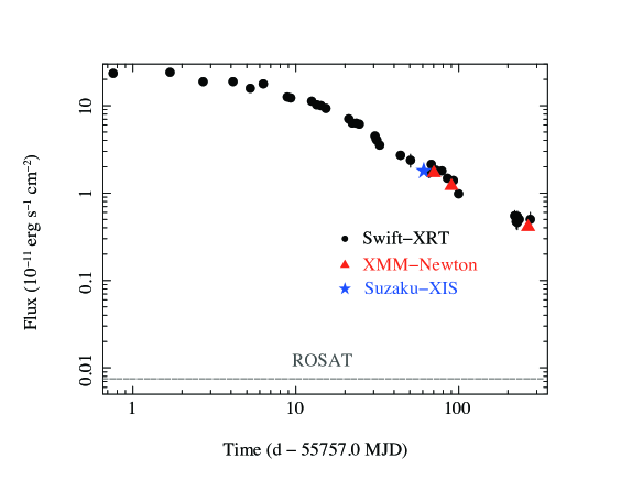
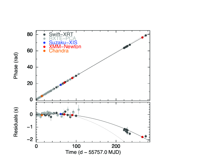
Figure 1.— Left panel: Flux decay of Swift J1822.3–1606  in the 1–10 keV energy range (see also Table 3). Right panel: pulse phase evolution as a function of time, together with the time residuals (lower panel) after having corrected for the linear component (correction to the $P$ value). The solid lines in the two panels mark the inferred $P$–$\dot{P}$ coherent solution based on the whole dataset, while the dotted lines represent the $P$–$\dot{P}$ coherent solution based on the data collected during the first 90 days only (see text for the details).

Table 1Swift J1822.3–1606  observations used for this work.

Instrument	Obs.ID	Datea	Exposure
		(MJD TBD)	(ks)
Swift/XRT	00032033001 (PC)	55 757.75058	1.6
RXTE/PCA	96048-02-01-00	55 758.48165	6.5
Swift/XRT	00032033002 (WT)	55 758.68430	2.0
Swift/XRT	00032033003 (WT)	55 759.69082	2.0
RXTE/PCA	96048-02-01-05	55 760.80853	1.7
Swift/XRT	00032033005 (WT)	55 761.54065	0.5
RXTE/PCA	96048-02-01-01	55 761.55969	5.0
Swift/XRT	00032033006 (WT)	55 762.24089	1.8
RXTE/PCA	96048-02-01-02	55 762.47384	4.9
Swift/XRT	00032033007 (WT)	55 763.30400	1.6
RXTE/PCA	96048-02-02-00	55 764.61846	6.1
RXTE/PCA	96048-02-02-01	55 765.46687	6.8
Swift/XRT	00032033008 (WT)	55 765.85252	2.2
Swift/XRT	00032033009 (WT)	55 766.28340	1.7
RXTE/PCA	96048-02-02-02	55 767.59064	3.0
RXTE/PCA	96048-02-02-03	55 769.35052	3.4
Swift/XRT	00032033010 (WT)	55 769.49531	2.1
Swift/XRT	00032033011 (WT)	55 770.39936	2.1
Chandra/HRC-I	13511	55 770.83049	11.7
Swift/XRT	00032033012 (WT)	55 771.23302	2.1
RXTE/PCA	96048-02-03-00	55 771.34185	6.8
Swift/XRT	00032033013 (WT)	55 772.40044	2.1
RXTE/PCA	96048-02-03-01	55 774.34999	6.9
RXTE/PCA	96048-02-03-02	55 777.85040	1.9
Swift/XRT	00032051001 (WT)	55 778.10744	1.7
Swift/XRT	00032051002 (WT)	55 779.18571	1.7
RXTE/PCA	96048-02-04-00	55 780.85040	6.7
Swift/XRT	00032051003 (WT)	55 780.49505	2.3
Swift/XRT	00032051004 (WT)	55 781.49878	2.3
RXTE/PCA	96048-02-04-01	55 782.57749	6.2
RXTE/PCA	96048-02-04-02	55 784.97179	6.2
Swift/XRT	00032051005 (WT)	55 786.42055	2.2
Swift/XRT	00032051006 (WT)	55 787.58688	2.2
RXTE/PCA	96048-02-05-00	55 788.05419	6.0
Swift/XRT	00032051007 (WT)	55 788.25617	2.3
Swift/XRT	00032051008 (WT)	55 789.66173	1.7
RXTE/PCA	96048-02-05-01	55 789.95880	6.0
Swift/XRT	00032051009 (WT)	55 790.36270	2.2
RXTE/PCA	96048-02-06-00	55 794.45899	6.5
RXTE/PCA	96048-02-07-00	55 799.61550	6.9
Swift/XRT	00032033015 (WT)	55 800.86278	2.9
Swift/XRT	00032033016 (WT)	55 807.48660	2.4
RXTE/PCA	96048-02-08-00	55 810.37979	6.0
Suzaku/XIS	906002010	55 817.92550	33.5
RXTE/PCA	96048-02-10-00	55 820.23970	6.7
Swift/XRT	00032033017 (WT)	55 822.82836	4.9
Swift/XRT	00032033018 (WT)	55 824.71484	1.5
RXTE/PCA	96048-02-10-01	55826.18540	5.6
XMM–Newton	0672281801	55 827.25350	10.6
Swift/XRT	00032033019 (WT)	55 829.45421	2.3
Swift/XRT	00032033020 (WT)	55 835.54036	2.6
RXTE/PCA	96048-02-11-00	55835.90370	7.0
Swift/XRT	00032033021 (WT)	55 842.06040	4.2
RXTE/PCA	96048-02-12-00	55842.23269	5.8
XMM–Newton	0672282701	55 847.06380	25.8
Swift/XRT	00032033022 (WT)	55 849.61916	3.4
RXTE/PCA	96048-02-13-00	55849.6597976	5.6
Swift/XRT	00032033024 (WT)	55 862.59155	10.2
RXTE/PCA	96048-02-14-00	55863.11100	5.6
Swift/XRT	00032033025 (PC)	55 977.16600	6.3
Swift/XRT	00032033026 (WT)	55 978.53399	10.2
Swift/XRT	00032033027 (PC)	55 981.99499	11.0
Swift/XRT	00032033028 (WT)	55 982.96299	7.0
Swift/XRT	00032033029 (WT)	55  985.17799	7.0
Swift/XRT	00032033030 (WT)	55  985.55000	7.0
Swift/XRT	00032033031 (WT)	55 991.09231	6.7
XMM–Newton	0672282901	56022.95692	26.9
Swift/XRT	00032033032 (WT)	56 031.141159	4.3

• Mid-point of the observations.

The broadband emission of these objects and their flaring activity are believed to be connected to their high dipolar and/or toroidal magnetic field: this is indeed supported by the measurement of surface dipolar $B$ field usually of the order of $10^{14}$–$10^{15}$ G (inferred through the assumption that, as ordinary pulsars, they are spun down via magnetic dipolar losses: $B\sim 3.2\times 10^{19}(P\dot{P})^{1/2}$ G, where $P$ is the spin period in seconds, $\dot{P}$ its first derivative and we assumed a neutron star mass and radius of $R\sim 10^{6}$ cm and $M\sim 1.4~{}M_{\odot}$, respectively). However, the recent detection of an SGR showing all the typical emission properties defining a magnetar (van der Horst et al., 2010; Esposito et al., 2010), but with an inferred dipolar surface magnetic field $<7.5\times 10^{12}$ G (Rea et al., 2010), has put into question the need of a high dipolar magnetic field (namely higher than the quantum electron critical field $B_{\rm Q}=m_{e}c^{2}/e\hbar\sim 4.4\times 10^{13}$ G ) for an object to show magnetar-like activity.

On 2011 July 14, a new SGR-like burst and associated outburst were discovered by the Swift  Burst Alert Telescope (BAT), and followed soon after by all X-ray satellites (Cummings et al., 2011). The fast slew of the Swift  X-ray telescope (XRT) promptly detected a new bright X-ray source at $\rm RA:18^{h}22^{m}18\fs 00$, $\rm Dec:-16\arcdeg 04^{\prime}26\farcs 8$ (J2000; $1\farcs 8$ error at a 90% confidence level; Pagani et al. 2011), with a spin period of $P\sim 8.43$ s (Göğüş & Kouveliotou, 2011). The lack of an optical/infrared counterpart (Bandyopadhyay et al., 2011; Rea et al., 2011b; de Ugarte Postigo & Munoz-Darias, 2011), as well as the characteristics of the bursts, the X-ray spin period and its spectral properties (Esposito et al., 2011a, b; Rea et al., 2011a), led to its identification as a new magnetar candidate (Cummings et al., 2011; Halpern, 2011).

After its discovery, many attempts were made to measure the spin period derivative of Swift J1822.3–1606 (Gogus et al., 2011; Kuiper & Hermsen, 2011; Livingstone et al., 2011) in order to estimate its surface dipolar field. We present here the timing and spectral results of the first 9 months of X-ray monitoring (§2 and §3) of the new magnetar candidate Swift J1822.3–1606, a detection of its quiescent counterpart in archival data (§4), as well as upper limits on its emission in the optical and radio bands (§5 and §6). A detailed study of the SGR-like bursts, precise X-ray position and pulse profile modeling will be reported elsewhere (Kouveliotou et al. in preparation). Using our timing and spectral results, we model the source outburst decay, and secular evolution, which resulted in an estimate of the its real age and crustal toroidal field (§7).

2. X-ray observations and data reduction

In this study, we used data obtained from different satellites (see Table 1 for a summary). Observations and data analysis are briefly described in the following.

2.1. Swift data

The X-Ray Telescope (XRT; Burrows et al. 2005) on-board Swift uses a front-illuminated CCD detector sensitive to photons between 0.2 and 10 keV. Two main readout modes are available: photon counting (PC) and windowed timing (WT). PC mode provides two dimensional imaging information and a 2.5073 s time resolution; in WT mode only one-dimensional imaging is preserved, achieving a time resolution of 1.766 ms.

The XRT data were uniformly processed with xrtpipeline (version 12, in the heasoft software package version 6.11), filtered and screened with standard criteria, correcting for effective area, dead columns, etc. The source counts were extracted within a 20-pixel radius (one XRT pixel corresponds to about $2\farcs 36$). For the spectroscopy, we used the spectral redistribution matrices in caldb (20091130; matrices version v013 and v014 for the PC and WT data, respectively), while the ancillary response files were generated with xrtmkarf, and they account for different extraction regions, vignetting and point-spread function corrections.

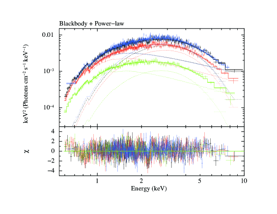
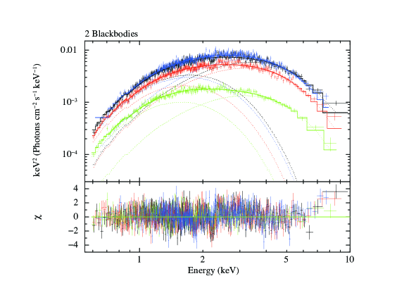
Figure 2.— Spectra of the Suzaku  (blue) and XMM–Newton  observations fitted together with a blackbody plus power-law and two-blackbody models (see text and Table 2 for details).

2.2. RXTE data

The Proportional Counter Array (PCA; Jahoda et al. 1996) on-board RXTE consists of five collimated xenon/methane multianode Proportional Counter Units (PCUs) operating in the 2–60 keV energy range. Raw data were reduced using the ftools package (version 6.11). To study the timing properties of Swift J1822.3–1606, we restricted our analysis to the data in Good Xenon mode, with a time resolution of 1 $\mu$s and 256 energy bins. The event-mode data were extracted in the 2–10 keV energy range from all active detectors (in a given observation) and all layers, and binned into light curves of 0.1 s resolution.

Table 2Spectral analysis of the Suzaku  and XMM–Newton  data.

			Blackbody $+$ Powerlaw			Two Blackbodies
Instrument	Timea	Fluxb	kT (keV)	RBB (km)c	$\Gamma$	kT1 (keV)	$R_{\rm BB1}$ (km)c	kT2 (keV)	$R_{\rm BB2}$ (km)c
Suzaku	60.93$\pm$0.48	1.78$\pm$0.01	0.678$\pm$0.008	1.2$\pm$0.1	2.90$\pm$0.04	0.39$\pm$0.01	2.6$\pm$0.4	0.79$\pm$0.01	0.9$\pm$0.1
XMM–Newton	70.25$\pm$0.06	1.70$\pm$0.01	0.689$\pm$0.006	1.1$\pm$0.1	2.86$\pm$0.03	0.40$\pm$0.01	2.6$\pm$0.4	0.84$\pm$0.01	0.8$\pm$0.1
XMM–Newton	90.06$\pm$0.11	1.20$\pm$0.03	0.679$\pm$0.005	1.0$\pm$0.1	2.99$\pm$0.03	0.37$\pm$0.02	2.5$\pm$0.4	0.79$\pm$0.01	0.7$\pm$0.1
XMM–Newton	266.1$\pm$0.2	0.4$\pm$0.1	0.623$\pm$0.008	0.61$\pm$0.08	3.05$\pm$0.04	0.35$\pm$0.01	2.0$\pm$0.2	0.78$\pm$0.01	0.4$\pm$0.1

• Times are calculated in days from MJD 55 757.0 .

• Fluxes are in units of $10^{-11}$erg s^-1cm^-2, referred to the BB+PL fit, and calculated in the 1–10 keV energy range. Errors in the table are given at 1$\sigma$ confidence level. Reduced $\chi^{2}$ and absorption values are $\chi^{2}_{\nu}/$dof =1.05/2522 and $N_{\rm H}=0.50(1)\times 10^{22}$cm^-2, $\chi^{2}_{\nu}/$dof =1.06/2522 and $N_{\rm H}=0.21(1)\times 10^{22}$cm^-2, for the BB+PL and BB+BB models, respectively.

• Radii are calculated assuming a distance of 5 kpc.

2.3. Suzaku data

Suzaku  (Mitsuda et al., 2007) observed the field of Swift J1822.3–1606  on 2012 September 13–14 with the pulsar located at the X-ray Imaging Spectrometer (XIS; Koyama et al. 2007) nominal position. The XIS consists of three front-illuminated (FI) CCD cameras (XIS0, XIS2 and XIS3), and one that is back-illuminated (BI; XIS1). One of the FI CCDs, XIS2, was not available at the time of our observation. XIS1 and XIS3 were operating in Normal Mode without any option (all the pixels on the CCD are read out every 8 s), while XIS0 was operating with the 1/8 Window option allowing a read out time of 1 s.

For each XIS, $3\times 3$ and $5\times 5$ edit modes cleaned event data were combined. Following standard practices, we excluded times within 436 s of Suzaku passing through the South Atlantic Anomaly and we also excluded the data when the line of sight was elevated above the Earth limb by less than $5^{\circ}$, or less than $20^{\circ}$ from the bright-Earth terminator. Moreover, we excluded time windows during which the spacecraft was passing through a cut-off rigidity of below 6 GV. Finally, we removed hot and flickering pixels. The resulting total effective exposure was $\sim$33.5 ks for each XIS. The SGR net count rates are 0.710(5), 1.180(6), and 1.060(6) count s^-1 in the XIS0, XIS1 and XIS3, respectively. For the spectral analysis, we used only XIS0 and XIS3, which are the best calibrated cameras, while for the timing analysis we made use only of the XIS0 data, which owing to the 1/8 Window option, have a timing resolution adequate to sample the pulsar spin period.

2.4. Chandra data

The Chandra  X-ray Observatory has observed Swift J1822.3–1606  with the High Resolution Imaging Camera (HRC–I; Zombeck et al. 1995) on 2011 July 28, for $\sim 12$ ks (ObsID: 13511). Data were analyzed using standard cleaning procedures and CIAO version 4.4. Photons were extracted from a circular region with a radius of 3^′′ around the source position, including more than 90% of the source photons (see Kouveliotou et al. 2012 in prep for further details on this observation). We inferred an effective HRC–I count-rate of $70\pm 1$ counts s^-1.

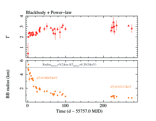
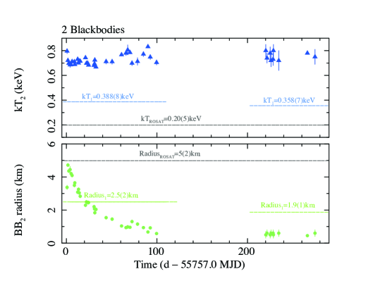
Figure 3.— Left panel: Spectral parameters for a blackbody plus power-law fit. Right panel: Spectral parameters for a two-blackbody fit (see text and Table 3 for details).

2.5. XMM-Newton data

We observed Swift J1822.3–1606  three time with XMM–Newton (Jansen et al., 2001) on 2011 September 23, October 12, and April 05, for $\sim$10, 25, and 27 ks, respectively. Only the second observation was partially affected by background flares which we have cleaned during our spectral analysis (see §3.1) resulting in a net exposure time of 19.4 ks. Data have been processed using SAS version 11, and we have employed the most updated calibration files available at the time the reduction was performed (April 2012). Standard data screening criteria are applied in the extraction of scientific products. For our analysis we used only the EPIC-pn camera, and we checked that the two MOS cameras gave consistent results. The EPIC-pn camera was set in Prime Large Window mode (timing resolution 48 ms), with the source at the aim-point of the camera. We have extracted the source photons from a circular region of 30^′′radius, and a similar region was chosen for the background in the same CCD but as far as possible from the source position. We restricted our analysis to photons having PATTERN$\leq$4 and FLAG=0. We find a EPIC-pn (background-subtracted) count rate of 5.03(3), 3.68(2) and 1.42(1) counts s^-1 for the first, second, and third observation, respectively.

Table 3Spectral analysis

			Blackbody $+$ Powerlaw∗		Two Blackbodies∗∗
ObsID	Timea	Fluxb	$\Gamma$	BB radius (km)c	kT2 (keV)	BB2 radius (km)c
33001	0.76$\pm$0.01	23.4$\pm$1.0	0.4$\pm$1.0	4.8$\pm$0.4	0.80$\pm$0.02	3.37$\pm$0.13
33002	1.69$\pm$0.01	24.1$\pm$0.5	2.0$\pm$0.1	5.4$\pm$0.1	0.72$\pm$0.01	4.7$\pm$0.1
33003	2.70$\pm$0.01	18.8$\pm$0.6	2.3$\pm$0.1	4.6$\pm$0.1	0.70$\pm$0.01	4.4$\pm$0.1
33005	4.11$\pm$0.01	18.8$\pm$0.6	2.4$\pm$0.1	3.3$\pm$0.4	0.68$\pm$0.02	4.4$\pm$0.2
33006	5.25$\pm$0.20	15.8$\pm$0.5	2.4$\pm$0.1	4.0$\pm$0.1	0.69$\pm$0.01	4.2$\pm$0.1
33007	6.31$\pm$0.08	17.8$\pm$0.7	2.1$\pm$0.1	4.2$\pm$0.1	0.71$\pm$0.01	4.1$\pm$0.1
33008	8.86$\pm$0.07	12.5$\pm$0.5	2.2$\pm$0.1	3.8$\pm$0.1	0.71$\pm$0.01	3.5$\pm$0.1
33009	9.29$\pm$0.04	12.2$\pm$0.4	2.4$\pm$0.1	3.4$\pm$0.1	0.69$\pm$0.01	3.6$\pm$0.1
33010	12.50$\pm$0.04	11.2$\pm$0.4	2.1$\pm$0.1	3.3$\pm$0.1	0.73$\pm$0.01	3.1$\pm$0.1
33011	13.40$\pm$0.07	10.2$\pm$0.3	2.4$\pm$0.1	3.4$\pm$0.1	0.70$\pm$0.01	3.2$\pm$0.1
33012	14.24$\pm$0.04	10.0$\pm$0.5	2.2$\pm$0.2	3.1$\pm$0.1	0.71$\pm$0.01	3.0$\pm$0.1
33013	15.27$\pm$0.01	9.3$\pm$0.1	2.2$\pm$0.1	2.3$\pm$0.1	0.71$\pm$0.01	2.8$\pm$0.1
51001	21.11$\pm$0.10	7.0$\pm$0.4	2.2$\pm$0.1	2.2$\pm$0.1	0.74$\pm$0.01	2.3$\pm$0.1
51002	22.19$\pm$0.16	6.3$\pm$0.3	2.4$\pm$0.1	2.0$\pm$0.2	0.70$\pm$0.01	2.5$\pm$0.1
51003	23.50$\pm$0.08	6.3$\pm$0.2	2.4$\pm$0.1	2.0$\pm$0.1	0.70$\pm$0.01	2.4$\pm$0.1
51004	24.50$\pm$0.14	6.1$\pm$0.3	2.3$\pm$0.1	1.5$\pm$0.2	0.68$\pm$0.01	2.4$\pm$0.1
51006	30.59$\pm$0.01	4.5$\pm$0.2	2.6$\pm$0.2	1.9$\pm$0.2	0.68$\pm$0.01	2.2$\pm$0.1
51007	31.07$\pm$0.07	4.1$\pm$0.2	2.7$\pm$0.2	2.0$\pm$0.1	0.69$\pm$0.02	2.1$\pm$0.1
51008	31.40$\pm$0.01	4.0$\pm$0.2	2.5$\pm$0.1	1.9$\pm$0.1	0.72$\pm$0.01	1.8$\pm$0.1
51009	32.67$\pm$0.01	3.5$\pm$0.3	2.9$\pm$0.1	1.8$\pm$0.2	0.67$\pm$0.01	2.0$\pm$0.1
33015	43.87$\pm$0.10	2.7$\pm$0.3	2.8$\pm$0.2	1.5$\pm$0.1	0.71$\pm$0.02	1.5$\pm$0.1
33016	50.49$\pm$0.31	2.4$\pm$0.4	3.0$\pm$0.3	1.6$\pm$0.1	0.71$\pm$0.02	1.4$\pm$0.1
6002010	60.93$\pm$0.48	1.78$\pm$0.03	2.85$\pm$0.03	1.30$\pm$0.01	0.77$\pm$0.01	1.03$\pm$0.02
33017	65.83$\pm$0.13	1.7$\pm$0.2	2.6$\pm$0.3	1.2$\pm$0.1	0.78$\pm$0.02	0.94$\pm$0.05
33018	67.72$\pm$0.20	2.1$\pm$0.2	2.3$\pm$0.2	1.0$\pm$0.1	0.81$\pm$0.04	1.0$\pm$0.1
81801	70.25$\pm$0.06	1.70$\pm$0.03	2.76$\pm$0.03	1.19$\pm$0.01	0.78$\pm$0.01	0.96$\pm$0.02
33019	72.45$\pm$0.35	1.8$\pm$0.1	2.3$\pm$0.6	1.5$\pm$0.1	0.70$\pm$0.02	1.3$\pm$0.1
33020	78.54$\pm$0.46	1.8$\pm$0.1	2.7$\pm$0.2	1.0$\pm$0.1	0.71$\pm$0.03	1.1$\pm$0.1
33021	85.06$\pm$0.38	1.48$\pm$0.15	2.4$\pm$0.6	1.4$\pm$0.1	0.77$\pm$0.02	0.94$\pm$0.06
82701	90.06$\pm$0.11	1.20$\pm$0.03	2.91$\pm$0.03	1.03$\pm$0.01	0.83$\pm$0.01	0.67$\pm$0.02
33022	92.62$\pm$0.38	1.4$\pm$0.1	3.1$\pm$0.2	1.2$\pm$0.1	0.75$\pm$0.02	0.92$\pm$0.07
33024	99.57$\pm$0.37	0.98$\pm$0.06	2.8$\pm$0.2	0.8$\pm$0.1	0.70$\pm$0.02	0.57$\pm$0.04
33025	220.2$\pm$0.8	0.55$\pm$0.08	2.6$\pm$0.2	0.8$\pm$0.1	0.80$\pm$0.05	0.5$\pm$0.2
33026	221.5$\pm$0.4	0.54$\pm$0.06	2.9$\pm$0.3	0.8$\pm$0.1	0.74$\pm$0.04	0.6$\pm$0.2
33027	225.0$\pm$0.1	0.47$\pm$0.08	2.9$\pm$0.4	0.9$\pm$0.1	0.78$\pm$0.05	0.5$\pm$0.2
33028	226.0$\pm$0.1	0.47$\pm$0.08	3.4$\pm$0.5	0.8$\pm$0.1	0.72$\pm$0.05	0.6$\pm$0.2
33029	228.2$\pm$0.1	0.46$\pm$0.08	3.0$\pm$0.5	0.9$\pm$0.1	0.73$\pm$0.05	0.6$\pm$0.2
33030	228.5$\pm$0.2	0.54$\pm$0.08	2.5$\pm$0.3	0.6$\pm$0.1	0.80$\pm$0.05	0.5$\pm$0.2
33031	234.5$\pm$0.4	0.50$\pm$0.08	3.1$\pm$0.5	0.8$\pm$0.1	0.72$\pm$0.08	0.6$\pm$0.2
82901	266.1$\pm$0.2	0.41$\pm$0.02	3.06$\pm$0.04	0.63$\pm$0.02	0.78$\pm$0.01	0.45$\pm$0.08
33032	274.5$\pm$0.4	0.5$\pm$0.1	2.8$\pm$0.4	0.6$\pm$0.1	0.75$\pm$0.06	0.6$\pm$0.2

• The absorption value and the blackbody temperature were fixed to be the same for all spectra of the first and second set: $N_{\rm H}=0.50(1)\times 10^{22}$cm^-2, $kT=0.660(8)$ keV and $kT=0.621(7)$ keV, for the first and second set of spectra, respectively. Reduced $\chi^{2}_{\nu}/$dof = 1.1/6501.

• The absorption value, blackbody temperature and radius were fixed to be the same for all spectra of the first and second set: $N_{\rm H}=0.21(1)\times 10^{22}$cm^-2, $kT_{1}=0.388(8)$ keV and BB₁ Radius = 2.5(1) km, and $kT_{1}=0.358(7)$ keV and BB₁ Radius = 1.9(1) km, for the first and second set of spectra, respectively. Reduced $\chi^{2}_{\nu}/$dof = 1.1/6542 .

• Times are calculated in days from MJD 55 757.0 .

• Fluxes are in units of $10^{-11}$erg s^-1cm^-2, referred to the BB+PL fit, and calculated in the 1–10 keV energy range. Errors in the table are given at 1$\sigma$ confidence level.

• Radii are calculated assuming a distance of 5 kpc.

3. Results of the X-ray monitoring

3.1. X-ray spectral modeling

Spectra were extracted as explained in §2, and rebinned in order to have at least 20 counts per bin in the Swift  spectra, and 50 counts per bin in the Suzaku  and XMM–Newton  spectra. We started our spectral analysis by fitting our higher quality spectra, those from the three XMM–Newton/pn, and Suzaku/XIS03 observations, with several models (using XSPEC version 12.7.0; see Figure 2 and Table 2). Best fits were found using a blackbody plus power-law (BB+PL; $\chi^{2}_{\nu}/$dof = 1.05/2522) and a 2 blackbodies (2BBs; $\chi^{2}_{\nu}/$dof = 1.06/2522) model, all corrected for the photoelectric absorption (phabs model with solar abundances assumed from Anders & Grevesse (1989) and photoelectric cross-section from Balucinska-Church & McCammon (1998)). The hydrogen column density along the line of sight was fixed to the same value for all of the spectra for a given model. We obtained N${}_{\rm H}=0.50(1)$ and $0.21(1)\times 10^{22}$cm^-2(errors in the text are at 1$\sigma$ level unless otherwise specified), for the BB+PL and 2BBs model, respectively (see Table 2). In Figure 2 we show the residuals of this spectral modeling, and note that, although statistically the fits can be considered equally good, the BB+BB model departs from the data at higher energies.

Already from this first analysis it is evident how the spectrum is changing in time, although very slowly.

We then expanded our spectral modeling by fitting simultaneously all the Swift/XRT, Suzaku/XIS03, and XMM–Newton/pn spectra. Again both models gave satisfactory fits (see Table 3). The hydrogen column density along the line of sight was fixed to the same values found from the modeling of our previous analysis. Table 3 summarizes the obtained spectral parameters.

For the BB+PL model, we first allowed all parameters to vary freely, and we noticed that the BB temperature was consistent with being constant in time in the early phases of the outburst (most probably changing too little for our spectral analysis to be sensible to its variations). This was visible already from Table 2 when considering only the most detailed spectra. We then tied the BB temperature across all spectra in the first 100 days of the outburst, and similarly we did for the last spectra (between 200-300 days after the trigger). Best fit (reduced $\chi^{2}_{\nu}/$dof = 1.1/6501) was found with a BB temperature of $kT=0.660(8)$ keV and $kT=0.621(7)$ keV, for the early and late times spectra, respectively. More detailed spectra would have certainly disentangled a slow decay between those two values. Figure 3 (left panel) shows the time evolution of the power-law index ($\Gamma$) and the BB area. We can see how the latter shrinks as the outburst decays, while the power law index increases slowly, anti-correlated with the X-ray flux (see also Figure 1 left panel).

On the other hand, for the BB+BB model we noticed that, by leaving all the parameters free to vary across all the spectra, the temperature and the radius of the first blackbody were not varying significantly in time. Similarly to the BB+PL case, we then fixed those values to be the same in all spectra at early and late times separately. This resulted in the best fit values of $kT_{1}=0.388(8)$ keV and BB Radius₁ = 2.5(1) km, and $kT_{1}=0.358(7)$ keV and BB Radius₁ = 1.9(1) km (to estimate the BB radii we assume a source distance of 5 kpc). The best fit had a reduced $\chi^{2}_{\nu}$/dof = 1.1/6542. The second blackbody has a relatively steady temperature around $\sim$0.7 keV (see Fig. 3 right panel) and its radius shrinks during the outburst decay.

In the late time spectra, taken $>$200 days after the outburst onset, the source flux decreases substantially (from $\sim 24$ to $0.4\times 10^{-11}$erg s^-1cm^-2), as the spectrum continues to soften.

We have also tried to model the spectra with a resonant cyclotron scattering model (Rea et al., 2007, 2008; Zane et al., 2009), and, although the fits gave a good chi-squared value ($\chi^{2}_{\nu}\sim$1.1/5912), the low magnetic field of Swift J1822.3–1606  (see §3.2) makes the use of those models, envisaged for $B\sim 10^{14}$ G, questionable (see also Turolla et al. 2011).

We note that, although the $\chi^{2}$ values of both the BB+PL and BB+BB fits might appear not acceptable from a purely statistical point of view, many systematic errors are present in the simultaneous spectral modeling of different satellites (the most severe being the uncertainties in the inter-calibration between them, which is believed to be within a 5% error). We did not add any systematic error in the spectral fitting to show the pure residuals of the fit; however, with only 5% systematic error, the reduced $\chi^{2}$ values would decrease substantially, reaching a fully acceptable fit for both models ($\chi^{2}_{\nu}\sim$1.0).

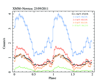
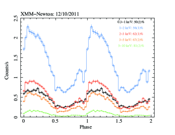
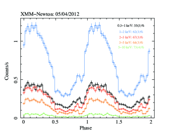
Figure 4.— Pulse profiles with 32 bins and relative pulsed fractions as a function of the energy band, for the three XMM–Newton  observations.

3.2. X-ray timing analysis

For the X-ray timing analysis we used all data listed in Table 1, after referring the event arrival times to the barycenter of the Solar System (assuming the source coordinates by Pagani et al. 2011 and the DE200 ephemeris for the Solar System). The first Swift/XRT event lists were used in order to start building up a phase coherent timing solution and to infer the SGR timing properties. We started by obtaining an accurate period measurement by folding the data from the first two XRT pointings which were separated by less than 1 day, and studying the phase evolution within these observations by means of a phase-fitting technique (see Dall’Osso et al. 2003 for details). Due to the possible time variability of the pulse shape we decided not to use a pulse template in the cross-correlation, which might artificially affect the phase shift, and we instead fit each individual folded light curve with two sine functions, the fundamental plus the first harmonic. In the following we also implicitly assume that the pulsation period (and its derivative) is a reliable estimate of the spin period (and its derivative), an assumption which is usually considered correct for isolated neutron stars.

The resulting best-fit period (reduced $\chi^{2}=1.1$ for 2 dof) is $P=8.43966(2)$ s (all errors are given at 1$\sigma$ c.l.) at the epoch MJD 55757.0 . The above period accuracy of 20 $\mu$s is enough to phase-connect coherently the later Swift, RXTE, Chandra, Suzaku, and XMM–Newton  pointings. The procedure was repeated by adding, each time, a further observation folded at the above period, and following the phase evolution of the ascending node of the fundamental sine function best fitting the profile of each observation. The relative phases were such that the signal phase evolution could be followed unambiguously for the whole visibility window until November 2011 (see Figure 1). When adding the RXTE  dataset, we also corrected the output phases by a small constant offset ($\sim$0.02), likely due to the different energy ranges and responses.

We modeled the phase evolution with a polynomial function with a linear plus quadratic term, the inclusion of the latter results in a significant improvement of the fit (an F-test gives a probability of $7\times 10^{-6}$ that the quadratic component inclusion is not required). The corresponding coherent solution (valid until November 2011) is $P=8.43772007(9)$ s and period derivative $\dot{P}=1.1(2)\times 10^{-13}$ s s^-1 ($\chi^{2}=132$ for 57 dof; at epoch MJD 55757.0). The above solution accuracy allows us to unambiguously extrapolate the phase evolution until the beginning of the next Swift visibility window which started in February 2012.

The final resulting phase-coherent solution (see also Table 4), once the latest 2012 observations are included, returns a best-fit period of $P=8.43772016(2)$ s and period derivative of $\dot{P}=8.3(2)\times 10^{-14}$ s s^-1 at MJD 55757.0 ($\chi^{2}=145$ for 67 dof; preliminary results were reported in Israel et al. 2012). The above best-fit values imply a surface dipolar magnetic field of $B\simeq 2.7\times 10^{13}$ G (at the equator), a characteristic age of $\tau_{\rm c}=P/2\dot{P}\simeq 1.6$ Myr, and a spin-down power L${}_{\rm rot}=4\pi I\dot{P}/P^{3}\simeq 1.7\times 10^{30}$ ${\rm erg\,s}^{-1}$(assuming a neutron star radius of 10 km and a mass of 1.4$M_{\odot}$).

The final solution has a relatively high r.m.s. ($\sim$ 120 ms) resulting in a best-fit reduced $\chi_{\nu}^{2}=2.1$. The introduction of high-order period derivatives in the fit of the phase evolution does not result in a significant improvement of the fit ($\chi^{2}=135$ for 66 dof; F-test gave a probability of $0.03$ that the cubic component inclusion is not required). This results in a 3$\sigma$ upper limit of the second derivative of the period of $\ddot{P}<5.8\times 10^{-21}$s s^-2 .

These values of $P$ and $\dot{P}$ are in agreement (within 1$\sigma$) with those inferred for the 2011 visibility window reported above However, this solution is not consistent, within $3\sigma$, with those already reported in the literature and based on a reduced dataset (Kuiper & Hermsen 2011; Livingstone et al. 2011; valid until 70 and 90 days from the onset of the outburst, respectively). In order to cross check our results and to compare them with those previously reported we fit only those observations of our dataset within about 90 days from the trigger. The corresponding best-fit parameters are $P=8.4377199(1)$ s and period derivative of $\dot{P}=1.6(4)\times 10^{-13}$ s s^-1 ($\chi^{2}=119$ for 52 dof; at epoch MJD 55757.0). The latter values are consistent with those of Livingstone et al. (2011).

This analysis together with the relatively high r.m.s. value suggest that the timing parameters of the pulsar are ”noisy”. Correspondingly, a timing solution based on a longer baseline may decrease the effect of a noisy behavior, while those reported earlier are likely affected by the shorter time-scale variability of the timing parameters.

In Figure 4 we show the pulse profiles as a function of energy for the three XMM–Newton  observations (see §2.5), folded with the best-fit timing solution reported above. We derived pulsed fractions (defined as $\rm{PF=[Max(counts/s)-Min(counts/s)]/[Max(counts/s})+$ $\rm{Min(counts/s)]}$) in the 0.3–1, 1–2, 2–3, 3–5, and 5–10 keV energy bands, of $47\pm 2$, $56\pm 1$, $65\pm 1$, $81\pm 1$, and $86\pm 2$ %, for the first observation; for the second observation: $50\pm 2$, $56\pm 1$, $62\pm 1$, $67\pm 2$, and $81\pm 2$ % ; and for the third observation: $55\pm 3$, $62\pm 3$, $67\pm 3$, $64\pm 3$, and $73\pm 4$% .

4. ROSAT pre-outburst observations

The Röntgensatellit (ROSAT) Position Sensitive Proportional Counter (PSPC; Pfeffermann et al. 1987) serendipitously observed the region of the sky including the position of Swift J1822.3–1606 between 1993 September 12 and 13 (obs. ID: rp500311n00), for an effective exposure time of 6.7 ks.

By means of a sliding cell source-detection algorithm, we found a 5.5$\sigma$ significant source with a 0.1–2.4 keV count rate of 0.012(3)counts s^-1 at the coordinates $\rm RA=18^{h}22^{m}18\fs 1,~{}Decl.=-16^{\circ}04^{\prime}26\farcs 4$ (positional uncertainty of 30^′′ radius at 90% c.l.; J2000). This source is also listed in the WGA and RXP catalogs, namely 1WGA J1822.2–1604 and 2RXP J182217.9–160417, with consistent values of count rate. The positions of the latter objects are $\sim$20^′′ and 10^′′ from the Swift-XRT position. Given the relatively large ROSAT/PSPC positional uncertainty, we believe the latter two sources and Swift J1822.3–1606  are the same object, which we propose as the SGR quiescent counterpart (see Figure 5).

We downloaded the relevant files of the ROSAT pointed observation and extracted the photon arrival times from a circle of $\sim 100^{\prime\prime}$ radius (corresponding to an encircled energy of $>$90%) around the X-ray position. We found that an absorbed blackbody with $N_{\rm H}$$<7\times 10^{21}$ cm^-2 (see also §3.1), $kT=0.20\pm 0.05$ keV, and a radius of $5\pm 2$ km, best fit the data (reduced $\chi^{2}=0.8$ for 4 degree of freedom). We infer an observed flux of $\approx 1.3\times 10^{-13}$ erg cm^-2 s^-1 and $\approx 4\times 10^{-14}$ erg cm^-2 s^-1 in the 0.1–2.4 keV and 1–10 keV energy ranges, respectively. Assuming a distance of 5 kpc, this flux results in a bolometric luminosity during the quiescence state of $L_{\rm qui}\sim 4\times 10^{32}$${\rm erg\,s}^{-1}$.

No significant periodic signal was found by means of a Fourier Transform, even restricting the search around the 8.44 s period. The 3$\sigma$ upper limits on the pulsed fraction (semi-amplitude of the sinusoid divided by the source average count rate) is larger than 100%.

Table 4Timing parameters for Swift J1822.3–1606.

Reference Epoch (MJD)	55757.0
Validity period (MJD)	55757– 56032
$P$ (s)	8.43772016(2)
$\dot{P}$ (s s-1)	$8.3(2)\times 10^{-14}$
$\ddot{P}$ (s s-2)	$<5.8\times 10^{-21}$
$\nu$ (Hz)	0.118515426(3)
$\dot{\nu}$(s-2)	$1.17(3)\times 10^{-15}$
$\ddot{\nu}$(Hz s-2)	$<8.1\times 10^{-23}$
$\chi^{2}/$dof	145/66
RMS residuals (ms)	120
B (Gauss)	$2.7\times 10^{13}$
Lrot (erg s-1)	$1.7\times 10^{30}$
$\tau_{\rm c}$ (Myr)	1.6

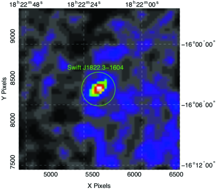
Figure 5.— ROSAT 1993 image of the region of Swift J1822.3–1606. The circle is centred at the Swift/XRT position.

         

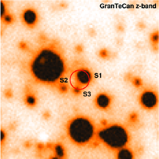
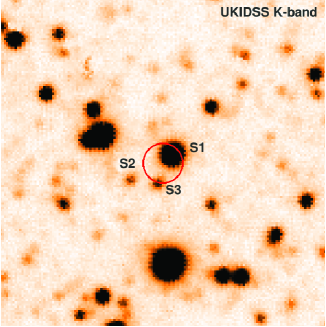
Figure 6.— Left panel: GranTeCan image of the Swift J1822.3–1606 field (30^′′$\times$ 30^′′) taken with the OSIRIS camera ($z$ band). The circle corresponds to the Swift/XRT position of the source (Pagani et al., 2011). The three objects detected close to, or within, the X-ray source error circle are labelled. Right panel: UKIRT image of the same area obtained with the WFC in the $K$ band.

5. Optical and infrared observations

We observed the field of Swift J1822.3–1606 with the 10.4-m Gran Telescopio Canarias (GranTeCan) at the Roque de los Muchachos Observatory (La Palma, Spain). Images were taken in service mode on 2011 July 21 with the OSIRIS camera, a two-chip Marconi CCD detector with a nominal un-vignetted $7\farcm 8\times 7\farcm 8$^′ field of view, and an unbinned pixel size of $0\farcs 125$. Observations were taken through the Sloan $z$ filter ($\lambda=969.4$  nm; $\Delta\lambda=261$  nm). We used a 5-point dithering pattern to correct for the effects of the CCD fringing in the Red part of the spectrum. We accurately selected the pointing of the telescope to position our target in the right CCD chip and a bright ($B\sim 10$) star $\sim$54^′′ East of it in the left one, in order to avoid the contamination from ghost images and saturation spikes. Unfortunately, the observations were taken in conditions of very high sky background due to the high lunar illumination, with the Moon phase at $\sim$0.5 and angular distance $\lesssim 90^{\circ}$, and with a seeing ranging from 1–$2\farcs 5$. Observations were taken using exposure times of 108 and 54 s, with the latter chosen to minimize the sky background induced by the Moon. The total integration time was 4100 s. We reduced the images with the dedicated tools in the IRAF ccdred package for bias subtraction and flat-fielding, using the provided bias and sky flat images. We performed the photometric calibration using exposures of the standard star PG  1528+0628. In order to achieve the highest signal–to–noise, we filtered out observations taken with the highest seeing and sky background. We aligned and co-added all the best-images by means of the swarp program (Bertin et al., 2002), applying a $3\sigma$ filter on the single pixel average to filter out residual hot and cold pixels and cosmic ray hits. We performed the astrometry calibration of the OSIRIS image with the WCStools astrometry package, using as a reference the coordinates of stars selected from the GSC2 catalogue (Lasker et al., 2008). Due to the significant and unmapped CCD distortions, we only obtained an rms of $0\farcs 3$ on the astrometric fit. We detected three objects (S1, S2, S3) within or close to the Swift J1822.3–1606  position (see also Rea et al. 2011b; Gorosabel et al. 2011). We computed their flux through standard aperture photometry using the IRAF package apphot. Their $z$-band magnitudes are $18.13\pm 0.16$, $20.05\pm 0.04$, and $19.94\pm 0.04$, for S1, S2 and S3, respectively (see Figure 5). We detected no other object consistent with the refined Swift/XRT position of Swift J1822.3–1606 (Pagani et al., 2011) down to a 3$\sigma$ limiting magnitude of $z=22.2\pm 0.2$. Given their bright optical magnitudes, we doubt that any of these objects is the optical counterpart to Swift J1822.3–1606. Based upon GranTecan spectroscopy, de Ugarte Postigo & Munos-Darias (2011) suggest that S1 and S2 are G to M-type stars.

As a reference, we inspected images of the Swift J1822.3–1606 field taken prior to our GranTeCan observations, i.e. when Swift J1822.3–1606 was probably in quiescence. To this aim, we searched for near-infrared (IR) observations taken as part of the UK Infrared Deep Sky Survey (UKIDSS; Lawrence et al. 2007), performed with the Wide Field Camera (WFCAM; Casali et al. 2007) at the UK Infrared Telescope (UKIRT) at the Mauna Kea Observatory (Hawaii). The Swift J1822.3–1606  field is indeed included in the UKIDSS Galactic Plane Survey (GPS) and data are available through Data Release 8 plus. Observations were taken on 2006 May 3rd (Bandyopadhyay et al., 2011). We downloaded the fully reduced, calibrated, and co-added $J$, $H$, $K$-band science images of the Swift J1822.3–1606  field produced by the UKIDSS pipeline (Hambly et al., 2008) together with the associated object catalogues through the WFCAM Science Archive (WSA) interface. The WFCAM astrometry is based on 2MASS (Skrutskie et al., 2006) and is usually accurate to $\sim 0\farcs 1$ (Lawrence et al., 2007). We clearly identified objects S1 ($J=13.92$; $H=12.37$; $K=11.62$), S2 ($J=16.62$; $H=15.75$; $K=15.20$), S3 ($J=16.43$; $H=15.40$; $K=14.88$) in the UKIDSS images (see Figure 5), with a relative flux comparable to the $z$-band flux measured on the OSIRIS ones. No other object is detected at the Swift J1822.3–1606 position down to $5\sigma$ limiting magnitudes of $J\sim 19.3$, $H\sim 18.3$ and $K\sim 17.3$.

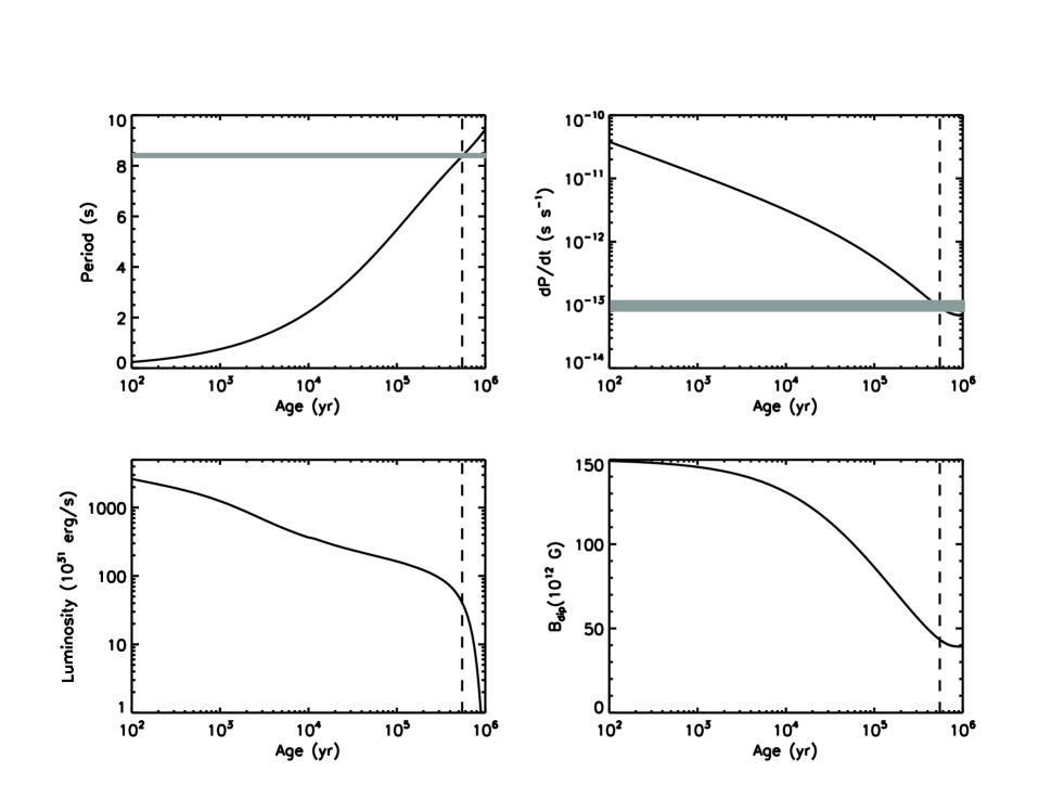
Figure 7.— From top left to bottom right, the evolution of the period, period derivative, luminosity, and surface dipole field, according to the model discussed in the text. Grey lines report on the current values of the Swift J1822.3–1606  period and period derivative (with its error). The vertical dashed lines mark the source ”real” age of 550 kyr .

Table 5GBT radio observations of Swift J1822.3–1606.

Date	Start time (MJD)	Exposure (s)	Smin (mJy)∗
2011-07-22	55764.26856481	1031.8269	0.06
2011-08-18	55792.00894675	967.3408	0.06
2011-09-20	55824.04596064	1365.0146	0.05
2011-10-19	55853.87988425	1375.7644	0.05

• S_min is the minimum flux density reached.

6. Radio observations

Radio observations of Swift J1822.3–1606  were performed at the 101 m Green Bank Telescope (GBT) on four occasions after the X-ray outburst, spaced by about a month one from the other (see Table 5). Data were acquired with the Green Bank Ultimate Pulsar Processing Instrument (GUPPI; DuPlain et al. 2008) at a central frequency of 2.0 GHz over a total observing bandwidth of 800 MHz.

For each observation, in order to correct for the dispersive effects of the interstellar medium, the bandwidth was split into 1024 channels about 250 of which were unusable because of radio frequency interferences (RFI), leaving us with 600 MHz of clean band. The observations lasted 16 to 23 minutes and were sampled every 0.6557 ms. Since the pulsar rotational parameters are known from X-ray observations (see §3.2), we first folded the data at the known period. We also folded the data at half, one third and a quarter of the nominal period in order to detect putative higher harmonics components of the intrinsic signal, in case the latter were deeply contaminated by RFI. Folding was done using dspsr (van Straten & Bailes, 2011) to form 30 s long sub-integrations subdivided into 512 time bins. The sub-integrations and the 1024 frequency channels, cleaned from RFI, were then searched around the nominal period $P$ and over a wide range of dispersion measure (DM) values (from 0 to 1000 pc cm^-3) to find the $P$–DM combination maximizing the signal-to-noise ratio. No dispersed signal was found in the data down to a flux of about 0.05 mJy depending on the observation (see Table 5).

Data were also blindly searched using the code suites presto and sigproc. In both cases, after de-dispersion of the data with 839 trial DMs (ranging from 0 to 1000 pc cm^-3) and removal of the frequency channels affected by RFI, the time series are transformed using fast Fourier algorithms and their power spectra searched for relevant peaks. These Fourier-based search techniques require a $2^{n}$ number of time samples in input; for this reason the amount of data analyzed was 1030 s, (a minute of fake data were added to the shortest observation) about two-thirds of the total of the longest observation, hence the flux limit attained, depending on the inverse of the square root of the integration time, was proportionally higher. With sigproc we also searched the data for single de-dispersed pulses but no signal was found in either the Fourier domain or the single pulse searches.

7. Discussion

7.1. The secular thermal evolution of Swift J1822.3–1606

To investigate whether the observed properties of Swift J1822.3–1606 are consistent with those of an evolved magnetar, as suggested by its characteristic age of $\tau_{\rm c}\simeq 1.6$ Myr, we followed the secular evolution of this object using a two-dimensional magneto-thermal evolution code. We refer to Pons et al. (2009) and Aguilera et al. (2008) for details about the code and the microphysical inputs of the model. This allows us to estimate the natal properties of the neutron star, its current age and internal field strength. We have considered the evolution, including magnetic field decay and heating by Ohmic diffusion, of an ultra-magnetized neutron star with a mass of 1.4 M_⊙, with no exotic phases nor fast neutrino cooling processes, but with enhanced neutrino emission from the breaking and formation of neutron and proton Cooper pairs (standard cooling scenario). We assumed an initial neutron star spin period of 10 ms and an initial dipolar field of $B_{\rm dip}(t=0)=1.5\times 10^{14}$ G. In Figure 7 we plot the evolution of spin period, period derivative, luminosity, and the dipolar surface magnetic field of a model that can match the current observed values at the “real” age of 550  kyr. The model has an initial crustal toroidal field that reaches a maximum value of $B_{\rm tor-max}(t=0)=7\times 10^{14}$  G (approximately half of the magnetic energy is stored in the toroidal component), which has now decayed to $B_{\rm tor-max}\sim 1.3\times 10^{14}$  G. We have also studied the expected outburst rate of this source, following the same procedure as in Perna & Pons (2011) and Pons & Perna (2011). We found that, at the present stage its outburst rate is very low ($\approx 10^{-3}$ yr^-1), because the magnetic field has been strongly dissipated.

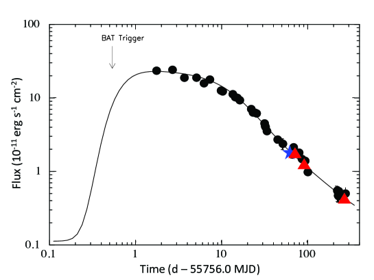
Figure 8.— Outburst model from Pons & Rea (2012) superimposed to the 1-10 keV flux decay of Swift J1822.3–1606  (see text for details).

7.2. The spectral evolution during the outburst

The spectral evolution during the outburst decay in Swift J1822.3–1606 bears resemblance to that observed in other magnetars in outburst, notably XTE J1810$-$197  (Halpern & Gotthelf, 2005; Bernardini et al., 2011), SGR 0501$+$4516  (Rea et al., 2009), CXOU J1647$-$4552  (Albano et al., 2010), and the “low field” SGR 0418$+$5729  (Esposito et al., 2010; Rea et al., 2010; Turolla et al., 2011). The decrease in flux appears, in fact, to be associated to a progressive spectral softening. Despite present data do not allow for an unambiguous spectral characterization over the entire outburst, evidence for a slow spectral softening is present in both the BB+BB and BB+PL models. In this respect we note that data are not consistent with a BB+PL fit in which the PL index is frozen to the same value in all observations (fitting the values of $\Gamma$ in Table 3 and Figure 3 with a constant function gives a reduced $\chi^{2}>10$).

A BB+PL spectrum is observed at soft X-ray energies in most magnetar sources, and is interpreted in terms of resonant cyclotron up-scattering of thermal surface photons by magnetospheric electrons in a twisted magnetosphere (e.g. Thompson et al. 2002; Nobili et al. 2008). In this framework, the evolution of Swift J1822.3–1606 is compatible with seed photons originating in a relatively small surface region which is heated by the (magnetic) event which gave rise to the outburst, magnetic energy release deep in the crust (as in Lyubarsky 2002) and/or ohmic dissipation of magnetospheric currents (Beloborodov, 2009). The heated region shrinks and cools progressively during the period covered by our observations (the equivalent BB radius decreased from $\sim 5$ km to $\sim 1$ km; in the following we always assume a 5 kpc distance) as residual heat is radiated away and the non-thermal component shows a progressive softening as the magnetosphere untwists.

On the other hand, the spectral evolution of the source can be also accommodated in the framework of a BB+BB spectral decomposition. In this model, the thermal emission is usually associated with two regions of different temperature and size which were heated during the outburst. It is well possible that a single heated region is actually produced, but with a meridional temperature gradient, which can be schematized as e.g. a hotter cap surrounded by a warm ring, similarly to the case of XTE J1810$-$197   (Perna & Gotthelf, 2008). The absence of a non-thermal tail is not in contrast with the twisted magnetosphere model if the twist is small and/or it affected only a limited bundle of closed field lines (see e.g. Esposito et al. 2010), especially if the surface field is low, as in the present source.

The archival ROSAT  observation show that, in quiescence, the source has a blackbody spectrum with $kT\sim 0.2$ keV and $R\sim 5$ km. Although the radius is somehow small, it is not unreasonable to associate the ROSAT  BB to thermal emission from the entire star surface, given the large errors and the uncertain distance determination.

If the outburst produced a heated region, which for concreteness we take to be a two-temperature cap, during the decay we witnessed a gradual shrinking of the hotter region (from $\sim 5$ km to $<1$ km). The warm ring also shrunk and cooled down slowly during the first 300 days after the outburst. Given the very slow spectral evolution of this component, we could obtain a good spectral modeling by fixing its temperature and radius to be constant during the first 100  days of the outburst, and again (at a different value) in the last 200-300 days (see Figure 3). This should be most probably interpreted as a gradual cooling which could not be followed in detail by the current observations, rather than a temperature jump.x

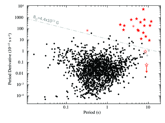
Figure 9.— Period–period derivative diagram for all known isolated pulsars. Black dots are radio pulsars (from the ATNF Catalog; Manchester et al. 2005), while red symbols are all known magnetars. Asterics denote PSR J1846$-$0258  and PSR 1622$-$4950, and empty stars are Swift J1822.3–1606  and SGR 0418$+$5729. Empty grey circles are the X-ray Dim Isolated Neutron Stars (XDINS: Turolla 2009). The dashed line represents the value of the critical electron magnetic field.

7.3. The outburst decay and timescales

The aggressive monitoring campaign we present here allowed us to study in detail the flux decay of Swift J1822.3–1606, and give an estimate of its typical timescale. Fitting the flux evolution in the first 225 days after the onset of the bursting activity, we found that an exponential function or a power law alone cannot fit the data properly, since at later time (50–80 days) the decay slope starts to change. We found an acceptable fit with an analytical function of the form $\mathrm{Flux}(t)=K_{1}+K_{2}e^{-(t/\tau)}+K_{3}t$ ($\chi^{2}$=4.7/37 dof); the best values of the parameters are $K_{1}=(1.76\pm 0.03)\times 10^{-11}$erg s^-1cm^-2, $K_{2}=(22.0\pm 0.3)\times 10^{-11}$erg s^-1cm^-2, $\tau=14.6\pm 0.3$ d, and $K_{3}=(-5.2\pm 0.2)\times 10^{-14}$erg s^-1cm^-2d^-1. The outburst decays of other magnetars are usually fitted by two components: an initial exponential or power-law component accounting for the very fast decrease in the first days or so (successfully observed only in very few cases), followed by a much flatter power-law (see Woods et al. 2004; Israel et al. 2007; Esposito et al. 2008). However, we note that the source has not reached the quiescent level yet; hence the modeling of the outburst, and relative timescale, might change slightly when adding further observations until the complete quiescent level is reached.

We have also compared the observed outburst decay with the more physical theoretical model presented in Pons & Rea (2012). We have performed numerical simulations with a 2D code designed to model the magneto-thermal evolution of neutron stars. The pre-outburst parameters are fixed by fitting the timing properties to the secular thermal evolution presented in section §7.1. We assume that Swift J1822.3–1606 is presently in an evolutionary state corresponding to that of the model presented in Figure 7 at an age of 550 kyr. We then model the outburst as the sudden release of energy in the crust, which is the progressively radiated away. We have run several of such models varying the total injected energy (between $10^{40}-10^{44}$ erg), as well as the affected volume, which are the two relevant parameters affecting the outburst decay (coupled with the initial conditions which were explored in §7.1). The depth at which the energy is injected and the injection rate bear less influence on the late-time outburst evolution (Pons & Rea 2012).

In Figure 8 we show our best representative model that reproduce the observed properties of the decay of Swift J1822.3–1606  outburst. This model corresponds to an injection of $4\times 10^{25}$ erg cm^-3 in the outer crust, in the narrow layer with density between $6\times 10^{8}$ and $6\times 10^{10}$ g cm^-3, and in an angular region of 35 degrees (0.6 rad) around the pole. The total injected energy was then $1.3\times 10^{42}$ erg .

However, we must note that this solution is not unique and the parameter space is degenerate. Equally acceptable solutions can be found varying the injection energy in the range $1-20\times 10^{25}$ erg cm^-3 and adjusting the other parameters. The outer limit (low density) of the injection region affects the timescale of the rise of the light curve, which is probably too fast (1-10 hours) to be observable in most of the cases. On the other hand, most of the light curve turns out to be insensitive to the inner limit (high density) of the injection region. Only the outburst tail (at $>50$ days) is affected by this parameter, but this effect is hard to be distinguished from similar effects from other microphysical inputs (e.g. varying the impurity content of the crust). Finally, variations of the angular size can be partially compensated by changes in the normalization factor which at present is undetermined (unknown distance). This changes the volume implied and therefore the estimate of the total energy injected. Thus we need to wait for the full return to quiescence, and combine our study with the complete analysis of the pulse profile and outburst spectrum, before we can place better constraints on the affected volume and energetics.

7.4. Radio and optical constraints

A recent study on the emission of radio magnetars has shown that all magnetars which exhibited radio pulsed emission, have a ratio of quiescent X-ray luminosity to spin-down power L${}_{\rm qui}/L_{\rm rot}<1$ (Rea et al., 2012). This suggests that the radio activity of magnetars and of radio pulsars might be due to the same basic physical mechanism, while its different observational properties are rather related to the different topology of the external magnetic field (e.g. a dipole and a twisted field; Thompson (2008).

In the case of Swift J1822.3–1606, inferring the quiescent (bolometric) and spin-down luminosities from our ROSAT data and our timing results (see §4 and §3.2), we derive L${}_{\rm qui}/L_{\rm rot}\simeq 4\times 10^{32}$ ${\rm erg\,s}^{-1}$$/1.7\times 10^{30}$ ${\rm erg\,s}^{-1}$$\simeq 235$ . This value is in line with the source not showing any radio emission (see Rea et al. 2012 for further details).

Concerning the optical and infrared observations, the bright optical fluxes of the sources S1–S3, much brighter than that of any other SGR in outburst for a comparable distance and interstellar extinction, as well as the lack of relative flux variability, suggest that objects S1–S3 are most likely unrelated to Swift J1822.3–1606. The hydrogen column density derived from the X-ray spectral fits ($N_{\rm H}=0.5\times 10^{22}$ cm^-2) corresponds to an interstellar extinction $E(B-V)\sim 0.89$ according to the relation of Predehl & Schmitt (1995). Using the wavelength-dependent extinction coefficients of Fitzpatrick (1999), this implies an absorption of $A_{z}\sim 1.33$ and $A_{K}\sim 0.32$ in the $z$ and $K$ band, respectively. Our OSIRIS upper limit would then correspond to an extinction-corrected spectral flux of $\lesssim 16.3\mu$Jy in the $z$ band, or to an integrated flux $\lesssim 1.36\times 10^{-14}$ erg cm^-2 s^-1. For an assumed Swift J1822.3–1606 distance of 5 kpc, this implies an optical luminosity $L_{z}\lesssim 4\times 10^{31}$ erg s^-1 during the outburst phase. Only very few magnetars are detected in the optical band, the only ones being 4U 0142$+$614, 1E 1048.1$-$5937, and SGR 0501$+$4516, all detected in the $I$ band (see, e.g. Mignani 2011; Dhillon et al. 2011). The optical flux of, e.g. 1E 1048.1$-$5937  during its recent flaring phase (Wang et al., 2008) corresponds to an $I$-band luminosity $L_{I}\sim(4\pm 2)\times 10^{30}$ erg s^-1 for an assumed distance of $3\pm 1$ kpc (Gaensler et al., 2005). Barring the difference in comparing fluxes obtained through two slightly different filters, our optical luminosity upper limit is about an order of magnitude above the 1E 1048.1$-$5937  luminosity. Similarly, the flux upper limit derived from the UKIDSS data implies for Swift J1822.3–1606 an IR luminosity $L_{K}\lesssim 1.1\times 10^{32}$  erg s^-1 during the quiescent phase. This upper limit is about an order of magnitude above the computed luminosities of the magnetars’ IR counterpart in quiescence and, therefore, it is not very constraining.

8. Conclusions

We have reported on the outburst evolution of the new magnetar Swift J1822.3–1606, which, despite its relatively low magnetic field ($B=2.7\times 10^{13}$ G), is in line with the outbursts observed for other magnetars with higher dipolar magnetic fields (similar energetics, flux evolution and spectral softening during the decay). Furthermore, we showed that the non detection in the radio band is in line with its high X-ray conversion efficiency ($L_{\rm qui}/L_{\rm rot}\simeq 235$; see also Rea et al. (2012) for further details).

We studied the secular thermal evolution of Swift J1822.3–1606  on the basis of the actual value of its period, period derivative and quiescent luminosity, and found that the current properties of the source can be reproduced if it has now an age of $\sim 550$ kyr, and it was born with a toroidal crustal field of $7\times 10^{14}$  G, which has by now decayed by less than an order of magnitude.

The position of Swift J1822.3–1606 in the $P$–$\dot{P}$ diagram (see Figure 9) is close to that of the “low” field magnetar SGR 0418$+$5729  (Rea et al., 2010). Although the fact that both have a sub-critical dipole field is not relevant per se, and the dipolar field in Swift J1822.3–1606 is at least four times higher than SGR 0418$+$5729, it is worth to stress that the discovery of a second magnetar-like source with a magnetic field in the radio-pulsar range strengthens the idea that magnetar-like behavior may be much more widespread than what believed in the past, and that it is related to the intensity and topology of the internal and surface toroidal components, rather than only to the surface dipolar field (Rea et al., 2010; Perna & Pons, 2011; Turolla et al., 2011).

Monitoring the source until its complete return to quiescence will be crucial to disentangle: 1) its complete spectral evolution during the outburst decay, 2) the possible presence of a second derivative of the rotational period, possibly due to the source timing noise, 3) refine further the modeling of the outburst and the surface region affected by this eruptive event.

References

- Aguilera et al. (2008) Aguilera, D. N., Pons, J. A., & Miralles, J. A. 2008, A&A, 486, 255
- Albano et al. (2010) Albano, A., Turolla, R., Israel, G. L., Zane, S., Nobili, L., & Stella, L. 2010, ApJ, 722, 788
- Anders & Grevesse (1989) Anders, E. & Grevesse, N., 1989, Geochimica et Cosmochimica Acta 53, 197
- Balucinska-Church & McCammon (1998) Balucinska-Church & McCammon, 1998, ApJ, 496, 1044
- Bandyopadhyay et al. (2011) Bandyopadhyay, R. M., Lucas, P. W., & Maccarone, T. 2011, Astron. Tel., 3502
- Beloborodov (2009) Beloborodov, A. M. 2009, ApJ, 703, 1044
- Bernardini et al. (2011) Bernardini, F., Perna, R., Gotthelf, E. G., Israel, G. L., Rea, N., & Stella, L. 2011, MNRAS, 418, 638
- Bertin et al. (2002) Bertin, E., Mellier, Y., Radovich, M., Missonnier, G., Didelon, P., & Morin, B. 2002, in Astronomical Society of the Pacific Conference Series, Vol. 281, Astronomical Data Analysis Software and Systems XI, ed. D. A. Bohlender, D. Durand, & T. H. Handley, 228
- Burrows et al. (2005) Burrows, D. N., et al. 2005, Space Science Reviews, 120, 165
- Casali et al. (2007) Casali, M., et al. 2007, A&A, 467, 777
- Cummings et al. (2011) Cummings, J. R., Burrows, D., Campana, S., Kennea, J. A., Krimm, H. A., Palmer, D. M., Sakamoto, T., & Zane, S. 2011, Astron. Tel., 3488
- Dall’Osso et al. (2003) Dall’Osso, S., Israel, G. L., Stella, L., Possenti, A., Perozzi, E. 2003, ApJ, 599, 485
- de Ugarte Postigo & Munoz-Darias (2011) de Ugarte Postigo, A. & Munoz-Darias, T. 2011, Astron. Tel., 3518
- Dhillon et al. (2011) Dhillon, V. S., et al. 2011, MNRAS, 416, L16
- DuPlain et al. (2008) DuPlain, R., Ransom, S., Demorest, P., Brandt, P., Ford, J., & Shelton, A. L. 2008, in Society of Photo-Optical Instrumentation Engineers (SPIE) Conference Series, Vol. 7019, Advanced Software and Control for Astronomy II, eds. Bridger, A. and Radzwill, N. Proceedings of the SPIE. SPIE, Bellingham WA, 70191D1–70191D10
- Esposito et al. (2010) Esposito, P., et al. 2010, MNRAS, 405, 1787
- Esposito et al. (2008) Esposito, P., et al. 2008, MNRAS, 390, L34
- Esposito et al. (2011a) Esposito, P., Rea, N., & Israel, G. L. 2011a, Astron. Tel., 3490
- Esposito et al. (2011b) Esposito, P., Rea, N., Israel, G. L., & Tiengo, A. 2011b, Astron. Tel., 3495
- Fitzpatrick (1999) Fitzpatrick, E. L. 1999, PASP, 111, 63
- Gaensler et al. (2005) Gaensler, B. M., McClure-Griffiths, N. M., Oey, M. S., Haverkorn, M., Dickey, J. M., & Green, A. J. 2005, ApJ, 620, L95
- Gavriil et al. (2002) Gavriil, F. P., Kaspi, V. M., & Woods, P. M. 2002, Nature, 419, 142
- Gogus et al. (2011) Gogus, E., Strohmayer, T., & Kouveliotou, C. 2011, Astron. Tel., 3503
- Gorosabel et al. (2011) Gorosabel, J., et al. 2011, Astron. Tel., 3496
- Göğüş & Kouveliotou (2011) Göğüş, E. & Kouveliotou, C. 2011, Astron. Tel., 3542
- Halpern & Gotthelf (2005) Halpern, J. P & Gotthelf, E. V., 2005, ApJ, 618, 874
- Halpern (2011) Halpern, J. P. 2011, GCN Circ., 12170
- Hambly et al. (2008) Hambly, N. C., et al. 2008, MNRAS, 384, 637
- Ibrahim et al. (2004) Ibrahim, A. I., et al. 2004, ApJ, 609, L21
- Israel et al. (2007) Israel, G. L., Campana, S., Dall’Osso, S., Muno, M. P., Cummings, J., Perna, R., & Stella, L. 2007, ApJ, 664, 448
- Israel et al. (2012) Israel, G. L., Esposito, P., Rea, N., Turolla, R., Zane, S., Mereghetti, S., & Tiengo, A. 2012, Astron. Tel., 3944
- Jahoda et al. (1996) Jahoda, K., Swank, J. H., Giles, A. B., Stark, M. J., Strohmayer, T., Zhang, W., & Morgan, E. H. 1996, in SPIE Conference Series, Bellingham WA, Vol. 2808, EUV, X-Ray, and Gamma-Ray Instrumentation for Astronomy VII., ed. O. H. W. Siegmund & M. A. Gummin, 59–70
- Jansen et al. (2001) Jansen, F., et al. 2001, A&A, 365, L1
- Kaspi et al. (2003) Kaspi, V. M., Gavriil, F. P., Woods, P. M., Jensen, J. B., Roberts, M. S. E., & Chakrabarty, D. 2003, ApJ, 588, L93
- Koyama et al. (2007) Koyama, K., et al. 2007, PASJ, 59, 23
- Kouveliotou et al. (2003) Kouveliotou, C., Eichler, D., Woods, P. M., et al. 2003, ApJ, 596, L79
- Kuiper & Hermsen (2011) Kuiper, L. & Hermsen, W. 2011, Astron. Tel., 3665
- Lasker et al. (2008) Lasker, B. M., et al. 2008, AJ, 136, 735
- Lawrence et al. (2007) Lawrence, A., et al. 2007, MNRAS, 379, 1599
- Livingstone et al. (2011) Livingstone, M. A., Scholz, P., Kaspi, V. M., Ng, C.-Y., & Gavriil, F. P. 2011, ApJ, 743, L38
- Lyubarsky (2002) Lyubarsky, Y. E. 2002, MNRAS, 332, 199
- Manchester et al. (2005) Manchester, R. N., Hobbs, G. B., Teoh, A., & Hobbs, M. 2005, AJ, 129, 1993
- Mereghetti (2008) Mereghetti, S. 2008, A&A Rev., 15, 225
- Mignani (2011) Mignani, R. P. 2011, Advances in Space Research, 47, 1281
- Mitsuda et al. (2007) Mitsuda, K., et al. 2007, PASJ, 59, 1
- Nobili et al. (2008) Nobili, L., Turolla, R., & Zane, S. 2008, MNRAS, 386, 1527
- Pagani et al. (2011) Pagani, C., Beardmore, A. P., & Kennea, J. A. 2011, Astron. Tel., 3493
- Perna & Gotthelf (2008) Perna, R. & Gotthelf, E. V., 2008, ApJ, 681, 522
- Perna & Pons (2011) Perna, R. & Pons, J.A., 2011, ApJ, 727, L51
- Pfeffermann et al. (1987) Pfeffermann, E., et al. 1987, in SPIE Conference Series, Bellingham, WA, Vol. 733, Soft X-ray optics and technology. Edited by E.-E. Koch & G. Schmahl, 519
- Pons et al. (2009) Pons, J. A., Miralles, J. A., & Geppert, U. 2009, A&A, 496, 207
- Pons & Perna (2011) Pons, J.A. & Perna, R. , 2011, ApJ, 741, L123
- Pons & Rea (2012) Pons, J. A. & Rea, N. 2012, ApJ, 750, L6
- Predehl & Schmitt (1995) Predehl, P. & Schmitt, J. H. M. M. 1995, A&A, 293, 889
- Rea & Esposito (2011) Rea, N. & Esposito, P. 2011, in High-Energy Emission from Pulsars and their Systems, ed. D. F. Torres & N. Rea, Astrophysics and Space Science Proceedings (Springer Berlin Heidelberg), 247–273
- Rea et al. (2011a) Rea, N., Esposito, P., Israel, G. L., Tiengo, A., & Zane, S. 2011a, Astron. Tel., 3501
- Rea et al. (2010) Rea, N., Esposito, P., Turolla, R., Israel, G. L., Zane, S., Stella, L., Mereghetti, S., Tiengo, A., Götz, D., Göğüş, E., & Kouveliotou, C. 2010, Science, 330, 944
- Rea et al. (2011b) Rea, N., Mignani, R. P., Israel, G. L., & Esposito, P. 2011b, Astron. Tel., 3515
- Rea et al. (2012) Rea, N., Pons, J. A., Torres, D. F., & Turolla, R. 2012, ApJ, 748, L12
- Rea et al. (2008) Rea, N., Zane, S., Turolla, R., Lyutikov, M. & Götz, D. 2008, ApJ, 686, 1245
- Rea et al. (2009) Rea, N., et al. 2009, MNRAS, 396, 2419
- Rea et al. (2007) Rea, N., Zane, S., Lyutikov, M. & Turolla, R. 2007, Ap&SS, 308, 505
- Skrutskie et al. (2006) Skrutskie, M. F., et al. 2006, AJ, 131, 1163
- Thompson (2008) Thompson, C. 2008, ApJ, 688, 499
- Thompson et al. (2002) Thompson, C., Lyutikov, M., & Kulkarni, S. R. 2002, ApJ, 574, 332
- Turolla (2009) Turolla, R. 2009, in Astrophysics and Space Science Library. Springer Berlin, Heidelberg, Vol. 357, Neutron stars and pulsars, ed. W. Becker, 141
- Turolla et al. (2011) Turolla, R., Zane, S., Pons, J. A., Esposito, P., & Rea, N. 2011, ApJ, 740, 105
- van der Horst et al. (2010) van der Horst, A. J., Connaughton, V., Kouveliotou, C, et al. 2010, ApJ, 711, L1
- van Straten & Bailes (2011) van Straten, W. & Bailes, M. 2011, PASA, 28, 1
- Voges et al. (1999) Voges, W., et al. 1999, A&A, 349, 389
- Wang et al. (2008) Wang, Z., Bassa, C., Kaspi, V. M., Bryant, J. J., & Morrell, N. 2008, ApJ, 679, 1443
- Woods et al. (2004) Woods, P. M., Kaspi, V. M., Thompson, C., Gavriil, F. P., Marshall, H. L., Chakrabarty, D., Flanagan, K., Heyl, J., & Hernquist, L. 2004, ApJ, 605, 378
- Zane et al. (2009) Zane, S., Rea, N., Turolla, R., & Nobili, L.. 2009, MNRAS, 398, 1403
- Zombeck et al. (1995) Zombeck, M. V., et al. 1995, SPIE, 2518, 96