From blockade to transparency: controllable photon transmission through a circuit QED system

Abstract

A strong photon-photon nonlinear interaction is a necessary condition for photon blockade. Moreover, this nonlinearity can also result a bistable behavior in the cavity field. We analyze the relation between detecting field and photon blockade in a superconducting circuit QED system, and show that photon blockade cannot occur when the detecting field is in the bistable regime. This photon blockade is the microwave-photonics analog of the Coulomb blockade. We further demonstrate that the photon transmission through such system can be controlled (from photon blockade to transparency) by the detecting field. Numerical calculations show that our proposal is experimentally realizable with current technology.

I Introduction

Superconducting circuit quantum electrodynamics (QED) allows studying the interaction between superconducting qubits (or superconducting artificial atoms) and quantized microwave fields (see, e.g., the reviews You11 ; Buluta11 ; Schoelkopf08 ). The coupling strengths have been explored from the strong-coupling regime to the ultrastrong one Bourassa09 ; Niemczyk10 ; Forn10 ; Ashhab10 . It is well known that the equally-spaced energy structure of the quantized microwave field can be changed to an anharmonic one, including dressed states Liu06 ; Wilson07 ; Wilson10 . The nonlinear energy splitting in circuit QED has been experimentally shown by the Rabi frequencies for different numbers of microwave quanta inside the cavity Hofheinz08 . Moreover, the experimental spectrum with the square root of the photon-number nonlinearity was reported Fink08 . Furthermore, the nonlinear response of the vacuum Rabi resonance was demonstrated Bishop09 .

Current experimental data indicate that the nonlinearity of the microwave photons can be many orders of magnitude larger than that of macroscopic media. These experiments Wilson07 ; Wilson10 ; Hofheinz08 ; Fink08 lay a solid foundation for developing microwave nonlinear interactions, which might be used to improve qubit readout Ginossar10 ; Boissonneault10 , and open the door to further study microwave nonlinear quantum optics at the level of single artificial atoms and single microwave photons. For example, the photon blockade phenomenon Imamoglu97 ; Birnbaum05 ; Faraon08 ; Miranowicz13 , where subsequent photons are prevented from resonantly entering a cavity, has recently been observed in circuit QED systems with resonant Lang11 and dispersive Hoffman11 qubit-cavity-field interactions.

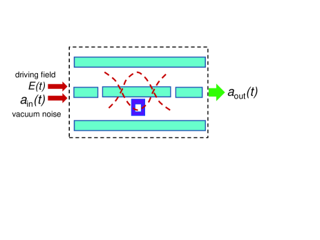
Figure 1: Schematic diagram for the circuit QED system of a superconducting charge qubit (denoted by the small purple square) coupled to a transmission line resonator, indicated by the black dashed box. The input (output) is denoted by the arrows going to (the arrow leaving from) the black dashed box. We assume that the input field, including the classical driving field $E(t)$ and the vacuum noise $a_{\rm in}(t)$, is applied to the cavity at the left port. The output field is measured at the right port.

Photon blockade originates from the anharmonic energy-level structure of the light field when the strong photon-photon interaction is induced by the nonlinear medium Imamoglu97 ; Miranowicz13 . In circuit QED systems in resonance, the anharmonicity of the microwave field is from a highly hybridization of the qubit and the microwave cavity field Lang11 . However, for the nonresonant case, the qubit can induce the photon-photon interaction when the qubit degrees of freedom are adiabatically eliminated Hoffman11 . This photon blockade is the analogue of Coulomb blockade Fulton87 , where single-electron transport, through a small metallic or semiconductor island sandwiched by two tunnel junctions in electron devices, occurs one by one due to the Coulomb interaction. Therefore, similar to the single-electron devices using the Coulomb blockade, the photon blockade could be used as a single-photon source or single-photon transistor.

One of the basic conditions for photon blockade is that the decay rate of the cavity field should be less than the photon-photon interacting strength. However, the decay of the photon-number states is very different from those of coherent states Lu89 ; Wang08 ; thus, photon blockade might not be observed when the photon number inside the cavity is extremely large. In addition, bistability is one of the basic properties of nonlinear systems, but there is a lack of studies on the effect of bistability on the photon blockade. Here we will study the relation between bistability and photon blockade and explore the possibility of unblocking the photon of the detecting field by using electromagnetically-induced transparency Liu12 ; Ian10 .

In our paper, we will first describe the model Hamiltonian in Sec. II, and also give detailed comparison between the photon and the Coulomb blockades. Then in Sec. III, we will study the relation between the bistability and the photon blockade. In Sec. IV, we will discuss the effect of the driving field on the photon blockade. In Sec. V, we will study how the photon blockade can be lifted and thus the system would become transparent. Finally, we summarize our results in Sec. VI.

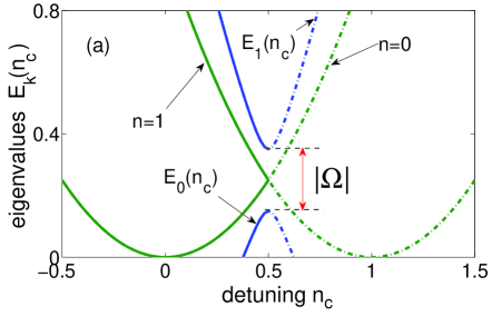
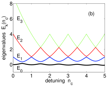
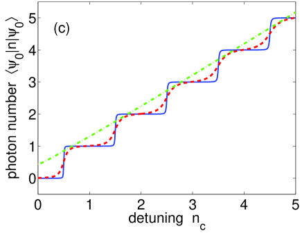
Figure 2: (Color online) (a) Eigenvalues $E_{k}(n_{c})$ (green curves) of the free Hamiltonian $\hbar\chi(n-n_{c})$ in Eq. (7) versus the rescaled detuning $n_{c}=(\chi-\Delta_{d})/(2\chi)$ for the photon numbers $n=0$ and $n=1$ inside the cavity, in energy units of $\hbar\chi$. Blue curves denote the eigenvalues $E_{0}(n_{c})$ and $E_{1}(n_{c})$ of the ground and first excited states for the Hamiltonian in Eq. (7) versus the rescaled detuning $n_{c}$ near the point $n_{c}=0.5$, with an effective Hamiltonian $\hbar\chi(n_{c}-0.5)(|1\rangle\langle 1|-|0\rangle\langle 0|)+\hbar(\Omega|1\rangle\langle 0|+\Omega^{*}|0\rangle\langle 1|)$, when the external field is included. The degeneracy of the two eigenvalues in the free Hamiltonian is lifted at the point $n_{c}=0.5$, with distance $\hbar|\Omega|$, by the external field. All dot-dashed curves mean $n_{c}>0.5$, however solid curves mean $n_{c}<0.5$. (b) Several eigenvalues $E_{k}(n_{c})$ (up to four) of the Hamiltonian in Eq. (7) versus the detuning $n_{c}$ for the ratio $\chi/|\Omega|=10$. (c) The mean photon number in the ground state $|\psi_{0}\rangle$ of the Hamiltonian in Eq. (7) versus the detuning $n_{c}$ for $\chi/|\Omega|=1$ (green dash-dotted curve), $10$ (red dashed curve), and $100$ (blue solid curve). This is the photon analog of the Coulomb staircase.

II Model Hamiltonian

As schematically shown in the black dashed box of Fig. 1, we study a circuit QED system in which the microwave cavity field with frequency $\omega_{0}$ inside the transmission line resonator, and the superconducting charge qubit with frequency $\omega_{q}$ are coupled to each other with the coupling strength $g$. We make the following assumptions:

(i) The cavity field and the qubit satisfy the large-detuning condition $|\omega_{0}-\omega_{q}|\gg g$. That is, they are in the dispersive interaction regime. Without loss of generality, hereafter we also assume $\Delta\equiv\omega_{0}-\omega_{q}>0$.

(ii) The rotating wave approximation can be used. In this case, the dynamics of the interaction Hamiltonian between the cavity field and the qubit can be easily solved.

(iii) Other upper levels of the qubit system are far from the first excited energy level, and the transition frequency between the first and second excited states is much bigger than the frequency of the cavity field. Thus, the cavity field only interacts with the qubit.

(iv) The circuit QED system is in the bad-cavity-limit, i.e., the decay rate of the microwave cavity field is much higher than that of the qubit.

The above conditions can be satisfied in circuit QED systems You11 ; Schoelkopf08 by well chosen sample design and fabrication. The interaction between the cavity field and the external environment, including the classical driving field and the vacuum noise, can be described via the input-output theory Walls94 .

Let us first neglect the vacuum noise and assume that a weak driving field $\varepsilon(t)$ is applied to the cavity; then the driven Hamiltonian

$$\widetilde{H}=\hbar\omega_{0}a^{\dagger}a+\hbar\frac{\omega_{q}}{2}\sigma_{z}+\hbar g(a^{\dagger}\sigma_{-}+a\sigma_{+})+\hbar[\varepsilon(t)a^{\dagger}+\text{H.c.}],$$ (1)

under the rotating wave approximation, can be transformed to an effective Hamiltonian $H=T^{\dagger}\widetilde{H}T$ with

$$H=\hbar\omega_{0}a^{\dagger}a+\frac{\hbar}{2}\left[\omega_{0}-E(N)\right]\sigma_{z}+\hbar\left[\varepsilon(t)a^{\dagger}+\varepsilon^{*}(t)a\right]$$ (2)

in the dispersive qubit-cavity-field interaction regime by applying a canonical transformation Compagno80

$$T=\exp\left[-\frac{\theta}{\sqrt{4N}}(a\sigma_{+}-a^{\dagger}\sigma_{-})\right],$$ (3)

with $\tan\theta=-2g\sqrt{N}/\Delta$ and

$$E(N)=\sqrt{\Delta^{2}+4g^{2}N}.$$ (4)

Here the total number operator $N$ of excitations of the qubit and the cavity field is given by

$$N=a^{\dagger}a+\frac{1}{2}(\sigma_{z}+1).$$ (5)

$a^{\dagger}$and $a$ are the creation and annihilation operators of the cavity field, respectively; $\sigma_{z}$ is Pauli’s operator, and $\sigma_{+}$ ($\sigma_{-}$) is the qubit raising (lowering) operator. In the derivation of Eq. (2), the terms proportion to $\textit{O}(N^{-1/2})$ are neglected.

The excited and ground states of the qubit with sign $\pm$ for $\sigma_{z}$ in the effective Hamiltonian in Eq. (2) are considered as the attractive and repulsive photon-photon interactions for $\Delta>0$. However, they are considered as the repulsive and attractive photon-photon interactions for $\Delta<0$.

We also assume that the cavity field and the qubit are in the strong-dispersive bad-cavity regime as in Refs. Hoffman11 ; Bishop10 . That is, the decay rate $\kappa$ of the microwave cavity field is much higher than the decay $\gamma$ and dephasing $\gamma_{\phi}$ rates of the qubit, and also satisfies the condition,

$$\gamma,\gamma_{\phi}\ll\kappa\ll\frac{g^{2}}{\Delta}\ll g\ll\Delta.$$ (6)

Thus, the environmental effect on the qubit can be neglected in our following discussions.

Table 1: Equivalence between photon and Coulomb blockades (or similarity between photon blockade and superconducting charge qubits).

Quanta	Photons	Electrons
Characteristic energy	Kerr energy $\hbar\chi$	Charging energy $E_{c}$
Energy offset control	Driving field frequency $\omega_{d}$	Gate voltage $V_{g}$
Detecting method	Driving field $E(t)$	Bias voltage $V_{b}$
Measurement of output	Photon number $\langle n\rangle$	Electron current $I$
Tunneling energy	Coupling energy $\hbar|\Omega|$	Josephson energy $E_{J}$

If a monochromatic driving field with frequency $\omega_{d}$ is applied to the cavity mode; then the Hamiltonian in Eq. (2) with $\varepsilon(t)=\Omega e^{-i\omega_{d}t}$ can be used to describe the photon blockade Imamoglu97 ; Liu12 when the coupling strength $\Omega$ between the driving field and the cavity field is much smaller than the photon-photon coupling constant $\chi$ given below. Moreover, the decay rate $\kappa$ of the cavity field should also be much smaller than $\chi$ to experimentally observe photon blockade. In the dispersive regime, the single two-level atom-induced photon blockade can be understood by expanding the Hamiltonian in Eq. (2), up to third order in the parameter $g/\Delta$, as

$$H_{\rm eff} = \hbar\chi(n-n_{\rm c})^{2}+\hbar(\Omega a^{\dagger}+\Omega^{*}a)$$ (7)

with $n=a^{\dagger}a$ in the rotating reference frame with the frequency $\omega_{d}$ for the driving field. Here, $\chi=g^{4}/\Delta^{3}$ denotes the photon-photon interaction strength, $n_{c}=(\chi-\Delta_{d})/(2\chi)$ is the rescaled detuning $\Delta_{d}=\omega_{0}-\omega_{d}$ between the driving and the cavity fields. We notice that an effective Hamiltonian as in Eq. (7) can also be derived for the case that the cavity field interacts with the multi-level superconducting quantum systems. The detailed derivations are in Ref. Boissonneault10 .

In the derivation of Eq. (7), we have used the weak-excitation condition $\Delta>2g\langle N\rangle$ for the photon blockade, also several constant terms and the qubit state-dependent cavity-frequency shift have been neglected with the assumption $\sigma_{z}=1$. That is, the qubit is in its excited state. Actually, the sign of the effective Hamiltonian in Eq. (7), derived from the Hamiltonian in Eq. (2), depends both on the qubit state and the detuning $\Delta$ between the qubit frequency $\omega_{q}$ and the cavity-field frequency $\omega_{q}$. In the following numerical discussions, we use our assumption $\Delta=\omega_{0}-\omega_{q}>0$ and $\sigma_{z}=1$ (the qubit is in the excited state). These selections are only used for the numerical calculations. These assumptions are equivalent to the case $\Delta<0$ and $\sigma_{z}=-1$ (when the qubit is in the ground state).

Equation (7) shows that the Kerr energy $\hbar\chi$ corresponds to the charging energy $E_{c}$, while the driving field frequency $\omega_{d}$ (or, equivalently, the rescaled detuning $n_{\rm c}$) corresponds to the gate voltage $V_{g}$ in single-electron devices for Coulomb blockade (see Table I). Equation (7) also shows that the parameters $\chi$, $\omega_{d}$ (or $n_{\rm c}$), and $|\Omega|$ play similar functions as the charging energy, the gate voltage, and the Josephson energy of the charge qubit, respectively. For resonant driving, $\Delta_{d}=0$ and $n_{\rm c}=0.5$, the photon states $|0\rangle$ and $|1\rangle$ are degenerate for the free Hamiltonian $\hbar\chi(n-0.5)^{2}$. As shown in Fig. 2(a), this degeneracy can be lifted by the coupling strength $|\Omega|$. Figures 2(b,c) show the variations of the eigenenergies and the mean photon number $\langle n\rangle$ of the ground state for the Hamiltonian in Eq. (7) as functions of the parameter $n_{\rm c}$. Variations for both the eigenenergy and the mean photon number are the same as those of the eigenenergy and mean charge number of charge qubits or single-electron devices for Coulomb blockade. The staircase shape for the mean photon number was experimentally demonstrated in circuit QED system Hoffman11 . Moreover, Fig. 2(a) also shows that a large ratio $\chi/|\Omega|$ corresponds to a sharper step. Namely, a weak driving field and strong photon-photon interaction are more useful for detecting photon blockade.

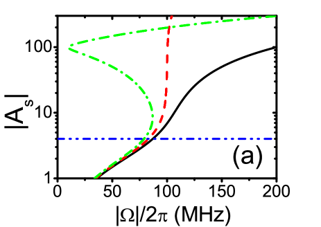
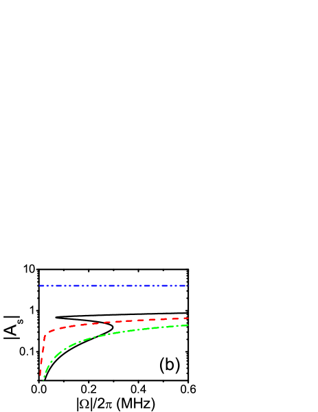
Figure 3: (Color online) Logarithm ${\rm log}(|A_{s}|)$ of the steady-state solution $|A_{s}|$ versus the strength of the driving field $|\Omega|$, for different detunings $\Delta_{d}/2\pi$ equal to: (a) $-1$ MHz (solid black), 0 MHz (dashed red) and 1 MHz (dot-dashed green), and (b) 36 MHz (solid black), 37 MHz (dashed red) and 38 MHz (dot-dashed green curves). Here, $N_{\rm up}$ (double-dot-dashed blue lines) is the upper bound photon number for the photon blockade, $\Delta/2\pi=1$ GHz, $\kappa/2\pi=0.1$ MHz, and $g/2\pi=200$ MHz. For the above-given parameters, $|A_{s}|$ has two stable states when $9.1\,{\rm kHz}<\Delta_{\rm d}<36.95\,{\rm MHz}$

III Bistability and blockade

We know that driven nonlinear photonic systems can exhibit bistability. To study the relation between bistability and photon blockade, we now write the equation of motion, using the driven Hamiltonian in Eq. (2) with $\varepsilon(t)=\Omega e^{-i\omega_{d}t}$, as

$$\frac{\partial a}{\partial t}=-\left[i\omega_{0}+\kappa-i\frac{g^{2}\sigma_{z}}{E(N)}\right]a-i\Omega e^{-i\omega_{d}t}-\sqrt{2\kappa}a_{\rm in}(t)$$ (8)

by using the relation $[a,f(a,a^{\dagger})]=\partial f(a,a^{\dagger})/\partial a^{\dagger}$ between the operator $a$ and the function $f(a,a^{\dagger})$ of the operators $a$ and $a^{\dagger}$. For example, we have the following relation

$$\left[a,\sqrt{\Delta^{2}+4g^{2}N}\right]=\frac{2g^{2}a}{\sqrt{\Delta^{2}+4g^{2}N}}.$$ (9)

Here, we have neglected the detailed derivation of the decay rate $\kappa$ and the quantum fluctuation $a_{\rm in}$ of the cavity field and phenomenologically added them to Eq. (8) according to Ref. Walls94 . As schematically shown in Fig. 1, we notice that the input includes both the quantum fluctuations $a_{\rm in}$ and the driving field $E(t)$. We assume that the quantum fluctuations $a_{\rm in}$ due to the vacuum field are Gaussian and have a zero mean value $\langle a_{\rm in}(t)\rangle=0$ and satisfy the Markov correlation

$$\langle a_{\rm in}(t)a^{\dagger}_{\rm in}(t^{\prime})\rangle=\delta(t-t^{\prime}).$$ (10)

If we denote $a(t)=A(t)e^{-i\omega_{d}t}$, then the steady-state solution $A_{s}\equiv\langle A\rangle_{s}$ for the cavity field becomes

$$A_{s}=-i\frac{\Omega}{\kappa+i[\Delta_{d}-g^{2}\sigma_{z}/E(\overline{N})]},$$ (11)

by setting $(\partial a/\partial t)=0$ in Eq. (8) and using the mean-field approximation, e.g., $\langle a^{\dagger}a\rangle_{s}=\langle a^{\dagger}\rangle_{s}\langle a\rangle_{s}$. We note in Eq. (11) and hereafter, although the operator $\sigma_{z}$ still remains in many equations, the operator $\sigma_{z}$ is actually set to $\sigma_{z}\equiv 1$ in all numerical calculations by assuming that the qubit is always in its excited state. In this case, the qubit, which is in the ground state, can also be easily discussed by setting $\sigma_{z}\equiv-1$. We also note that $E(\overline{N})$ in Eq. (11) is the expression of $E(N)$ when replacing the operator $a^{\dagger}a=N$ by the steady-state value $\overline{N}=|A_{s}|^{2}$, i.e.,

$$E(\overline{N})=\sqrt{\Delta^{2}+4g^{2}\left[|A_{s}|^{2}+\frac{1}{2}(1+\sigma_{z})\right]}.$$ (12)

Equation (11) shows that the cavity-field amplitude $|A_{s}|^{2}$ has two stable states when $\Delta_{d}$ satisfies the condition

$$\Delta_{-}<\Delta_{d}<\Delta_{+},$$ (13)

with

$$\Delta_{\pm}=\frac{g^{2}}{E(\overline{N})}-\frac{2g^{4}|A_{s}|^{2}\mp\sqrt{4g^{8}|A_{s}|^{4}-\kappa^{2}E^{6}(\overline{N})}}{E^{3}(\overline{N})}.$$ (14)

Equation (11) also clearly shows when the qubit is decoupled from the cavity field (i.e., $g=0$) or when the driving field makes $|A_{s}|^{2}$ extremely large, such that $g\sigma_{z}/E(\overline{N})\approx 0$, then the response of the system is the same as that of the harmonic oscillator. However, when $g\neq 0$, the resonant peak of $|A_{s}|^{2}$ will move to $\omega_{d}=\omega_{0}-g\sigma_{z}/E(\overline{N})$. That is, when the cavity contains $|A_{s}|^{2}$ photons, the frequency $\omega_{d}$ of the driving field should be increased an amount $-g\sigma_{z}/E(\overline{N})$ to overcome the photon blockade Imamoglu97 . The upper-bound photon number inside the cavity for the photon blockade is

$$N_{\rm up}\;\sim\;\frac{g^{4}}{\Delta^{3}\kappa}\;=\;\frac{\chi}{\kappa}$$ (15)

in the dispersive regime, as discussed in Ref. Bishop10 .

In Fig. 3, the steady-state $|A_{s}|$ versus the input $|\Omega|$ is plotted for several different detunings $\Delta_{d}$ and other experimentally accessible parameters Hoffman11 . Figure 3 clearly shows that the bistability disappears for either $\Delta_{d}>\Delta_{+}$ or $\Delta_{d}<\Delta_{-}$. Figure 3 also shows that most values for $|A_{s}|$ are smaller than the upper bound value $\sqrt{N_{\rm up}}$ for some values of $\Delta_{d}$ in the bistable regime, e.g., values in the region near $\Delta_{d}/2\pi=37$ MHz, as shown in Fig. 3(b). However, as shown in Fig. 3 (a) for other parameter regimes of $\Delta_{d}$, we find that the upper bound value $\sqrt{N_{\rm up}}$ can be smaller than some values of $|A_{s}|$ corresponding to the lower branch of the bistable curve. Therefore, Fig. 3 tells us that $N_{\rm up}$ is a necessary but not sufficient condition for photon blockade. Because one input corresponds to two stable outputs in the hysteresis region, thus the photon blockade is not well defined in such region.

Figure 4: (Color online) (a) Coherence $g^{(2)}(0)$ versus the driving field strength $|\Omega|$. (b) $g^{(2)}(\tau)$ versus the delay time $\tau$, where the solid-black and dashed-red curves correspond to the driving strengths $|\Omega|/2\pi=0.01$ MHz and 1 MHz, respectively. Also, $\Delta_{d}=38.5$ MHz, $\Delta/2\pi=1$ GHz, $g/2\pi=200$ MHz, and $\kappa/2\pi=0.1$ MHz. Also, $g^{(2)}(0)$ versus the detuning $\Delta_{d}$ in: (c) for $g/2\pi=100$ MHz and (d) for $g/2\pi=200$ MHz; with $\Delta/2\pi=1$ GHz, $|\Omega|/2\pi=0.01$ MHz, and $\kappa/2\pi=0.1$ MHz. For parameters given in (c) and (d), the condition of stable states for the driving field is $18\,{\rm kHz}<\Delta_{\rm d}<9.627\,{\rm MHz}$ and $9.1\,{\rm kHz}<\Delta_{\rm d}<36.95\,{\rm MHz}$, respectively.

IV Dependence of photon blockade on detuning $\Delta_{d}$ and driving strength $\Omega$

To show the effect of the driving field on the photon blockade, let us now study the statistical properties of the cavity field when the input $a_{\rm in}$ of the vacuum fields in Eq. (8) is considered. We assume that the vacuum fields $a_{\rm in}$ in Eq. (8) result in a small fluctuation $A_{f}(t)$ of the cavity field near its stable steady-state $A_{s}$ by writing the cavity operator as

$$A(t)=A_{s}+A_{f}(t).$$ (16)

In addition to the steady-state solution as in Eq. (11), with the input $a_{\rm in}(t)=A_{\rm in}(t)e^{-i\omega_{d}t}$, we can obtain an equation of motion for the fluctuation operator $A_{f}(t)$ as

$$\frac{\partial A_{f}(t)}{\partial t}=-\big{[}i\widetilde{\Delta}_{d}(\overline{N})+\kappa\big{]}A_{f}(t)-i\alpha(\overline{N})A^{\dagger}_{f}(t)-\sqrt{2\kappa}A_{\rm in}(t)$$ (17)

with

$$\widetilde{\Delta}_{d}(\overline{N})=\Delta_{d}-\delta\omega(\overline{N}),$$ (18)

$$\alpha(\overline{N})=2\frac{g^{4}A^{2}_{s}\sigma_{z}}{E^{3}(\overline{N})},$$ (19)

and

$$\delta\omega(\overline{N})=\frac{g^{2}\sigma_{z}}{E^{3}(\overline{N})}\left[E^{2}(\overline{N})-2g^{2}|A_{s}|^{2}\right].$$ (20)

Here the terms with higher orders of $A_{f}(t)$ and $A_{f}^{\dagger}(t)$, e.g., the term $A_{f}(t)A_{f}(t)$, have been neglected. By applying the Fourier transform

$$A_{f}(t)=\int_{-\infty}^{\infty}\frac{d\omega}{\sqrt{2\pi}}\exp(-i\omega t)A_{f}(\omega)$$ (21)

and also using the conjugate of Eq. (17) with $A^{\dagger}_{f}(\omega)\equiv[A_{f}(-\omega)]^{\dagger}$, we obtain the solution of the fluctuation as

$$A_{f}(\omega)=\frac{i\sqrt{2\kappa}}{d(\omega)}\left[\left(\widetilde{\Delta}_{\rm d}-\omega+i\kappa\right)A_{\rm in}(\omega)+\alpha(\overline{N})A^{\dagger}_{\rm in}(\omega)\right]$$ (22)

with the denominator factor

$$d(\omega)=(i\omega+\kappa)^{2}+\widetilde{\Delta}^{2}_{d}-|\alpha(\overline{N})|^{2}.$$ (23)

The statistical properties of the cavity field can be described via the second-order degree of coherence $g^{(2)}(\tau)$. Because we assume that the vacuum input is Gaussian and satisfies the Markov correlation, thus $g^{(2)}(\tau)$ can be obtained by just calculating the correlation function with two operators using Wick’s theorem, that is

$$g^{(2)}(\tau) = \frac{2{\rm Re}[A_{s}^{2}\langle A_{f}^{\dagger}(t)A^{\dagger}_{f}(t^{\prime})\rangle+|A_{s}|^{2}\langle A^{\dagger}_{f}(t)A_{f}(t^{\prime})\rangle]}{(|A_{s}|^{2}+\langle n_{f}(t)\rangle)^{2}}$$ (24)

$$+ \frac{|\langle A_{f}^{\dagger}(t)A^{\dagger}_{f}(t^{\prime})\rangle|^{2}+|\langle A^{\dagger}_{f}(t^{\prime})A_{f}(t)\rangle|^{2}}{(|A_{s}|^{2}+\langle n_{f}(t)\rangle)^{2}}+1$$

with $t^{\prime}=t+\tau$ and $\langle n_{f}(t)\rangle=\langle A^{\dagger}_{f}(t)A_{f}(t)\rangle$.

It is easy to obtain $g^{(2)}(\tau)$ straightforwardly by calculating all correlation functions in Eq. (24) using Eq. (22) and $[A_{f}(-\omega)]^{\dagger}$. The second-order degrees of coherence $g^{(2)}(0)$ and $g^{(2)}(\tau)$ are plotted in Figs. 4(a,b) using experimentally-accessible parameters, e.g., in Ref. Hoffman11 . Figures 4(a,b) show that the cavity field tends to the classical behavior when increasing the strength $\Omega$. In this case, the photons might not be blockaded and can transparently pass through the circuit QED system. To explore the effect of the frequency of the driving field, $g^{(2)}(0)$ is plotted as a function of the detuning $\Delta_{d}$ in Figs. 4(c,d) for different coupling strengths between the qubit and the cavity field with other parameters given in the caption of Fig. 4. Figures 4(c,d) clearly demonstrate that the nonclassical behavior of the cavity field is out of the bistable regime for detuning $\Delta_{d}$. For example, Fig. 4(c) shows $g^{(2)}(0)\leq 1$ when $\Delta_{d}/2\pi\geq 9.85$ MHz, which is larger than the upper bound value $9.627$ MHz of $\Delta_{d}$ for the bistabilility, and thus the photon blockade cannot occur in the bistable regime.

V Photon blockade and transparency

To further discuss properties of the light field transmission when the photons are blockaded, we now study the response of the circuit QED system to the vacuum input field, which can be considered as a weak detecting field. According to the input-output theory Walls94 , the output field can be expressed as

$$a_{\rm out}(t)=\sqrt{2\kappa}a(t)+a_{\rm in}(t)+i\frac{\Omega}{\sqrt{2\kappa}}\exp(-i\omega_{d}t)$$ (25)

by using the cavity field and the input fields. From the former study, we know

$$a(t)=A(t)\exp(-i\omega_{d}t)=\left[A_{s}+A_{f}(t)\right]\exp(-i\omega_{d}t).$$ (26)

Thus, the Fourier components of the output field can be written as

$$a_{\rm out}(\omega)=A_{\rm in}(\omega^{\prime})+\sqrt{2\kappa}A_{f}(\omega^{\prime})+\left[\frac{2\kappa A_{s}+i\Omega}{\sqrt{2\kappa}}\right]\delta(\omega^{\prime}),$$ (27)

with $\omega^{\prime}=\omega+\omega_{d}$ and $A_{f}(\omega)$ given in Eq. (22). The physical meaning becomes clear if the vacuum input $a_{\rm in}(t)$ is assumed as a single-mode field $a_{\rm in}(t)=\xi\exp(-i\omega t)$ with the real parameter $\xi\ll|\Omega|$; that is, this weak detecting field does not change the statistical properties of the cavity field. In this case, $\omega^{\prime}$ in Eq. (27) is changed to $\omega^{\prime}=\omega_{d}-\omega$, and the terms $A_{\rm in}(\omega^{\prime})$ and $\delta(\omega^{\prime})$ in Eq. (27) denote the response of the system to the input vacuum field and the classical driving field, respectively. However, the term with $A^{\dagger}_{\rm in}(\omega^{\prime})$ exhibits four-wave mixing with frequency $\omega-2\omega_{d}$, which will be studied elsewhere.

The coefficient of $A_{\rm in}(\omega^{\prime})$ for the output in Eq. (27) corresponds to that of $A_{\rm in}(\omega^{\prime})$ in the expression $A_{f}(\omega^{\prime})$ of Eq. (22) plus one. Thus, in Figs. 5(a,b), the real $A_{\rm R}(\omega^{\prime})$ and imaginary $A_{\rm I}(\omega^{\prime})$ parts for the normalized coefficient of $A_{\rm in}(\omega^{\prime})/\xi$ in Eq. (22) for $A_{\rm in}(t)=\xi\exp[-i(\omega-\omega_{d})t]$ are plotted using the same parameters as in Fig. 4(c), with $\Delta_{d}\approx 9.96$ MHz and $\Delta_{d}\approx 9.74$ MHz. These two values correspond to the minimum (photon blockade) and the maximum (classical case) of $g^{(2)}(0)$ in Fig. 4(c). As expected, we find that the response of the circuit QED system to the input field (or, say, weak-detecting field) has a Lorentzian shape, which is the same as the decay spectrum of the single photon, when the photon is blockaded. However, the weak detecting field shows transparency windows to the circuit QED system when the driving field is changed such that the cavity field is in the classical regime (or the photon is not blockaded). Thus, we can control the photon (from blockade to transparency) by changing the applied classical field.

Figure 5: (Color online) The real $A_{\rm R}(\omega^{\prime})$ and imaginary $A_{\rm I}(\omega^{\prime})$ parts $A_{\rm in}(\omega^{\prime})/\xi$ as a function of $\omega^{\prime}=\omega_{d}-\omega$ are plotted in (a) and (b), respectively, for the detuning $\Delta_{d}/2\pi$ equal to 9.74 MHz (solid black curves) and 9.96 MHz (dashed red curves) assuming $\Delta/2\pi=1\,$GHz, $g/2\pi=100\,$MHz, and $\kappa/2\pi=|\Omega|/2\pi=0.1\,$MHz.

VI Conclusions

In summary, we have studied the tunable transmission from the photon blockade to the photon transparency in superconducting circuit QED systems when the interaction between the qubit and the cavity field is in the dispersive regime. We analyze the effect of the driving field on the photon blockade. We also show the relation between the optical bistability and the photon blockade. We find that the photon blockade can be controlled by a classical driving field, that is, the photon blockade strongly depends on the properties of the driving field. We also find that the circuit QED system can be used to generate a four-wave mixing signal. All parameters in our numerical calculations are taken from experimentally available data. Therefore, our study should be experimentally realizable with current technology. We finally point out that the similarity between the photon blockade and Coulomb blockade (or superconducting charge qubit) makes it possible to simulate the electron behavior (or Josephson effect) using photonic devices.

VII Acknowledgement

Y.X.L. is supported by the National Natural Science Foundation of China under Grant Nos. 61025022, 91321208, and the National Basic Research Program of China Grant No. 2014CB921401. A.M. is supported by Grant No. DEC-2011/03/B/ST2/01903 of the Polish National Science Centre. F.N. is partially supported by the RIKEN iTHES Project, MURI Center for Dynamic Magneto-Optics, JSPS-RFBR contract No. 12-02-92100, Grant-in-Aid for Scientific Research (S), MEXT Kakenhi on Quantum Cybernetics, and the JSPS via its FIRST program.

References

- (1) J. Q. You and F. Nori, Phys. Today 58(11), 42 (2005); Nature (London) 474, 589 (2011).
- (2) I. Buluta, S. Ashhab, and F. Nori, Rep. Prog. Phys. 74, 104401 (2011).
- (3) R. J. Schoelkopf and S. M. Girvin, Nature (London) 451, 664 (2008).
- (4) J. Bourassa, J. M. Gambetta, A. A. Abdumalikov, Jr., O. Astafiev, Y. Nakamura, and A. Blais, Phys. Rev. A 80, 032109 (2009).
- (5) T. Niemczyk, F. Deppe, H. Huebl, E. P. Menzel, F. Hocke, M. J. Schwarz, J. J. Garcia-Ripoll, D. Zueco, T. Hümmer, E. Solano, A. Marx, and R. Gross, Nat. Phys. 6, 772 (2010).
- (6) P. Forn-Diaz, J. Lisenfeld, D. Marcos, J. J. Garcia-Ripoll, E. Solano, C. J. P. M. Harmans, and J. E. Mooij, Phys. Rev. Lett. 105, 237001 (2010).
- (7) S. Ashhab and F. Nori, Phys. Rev. A 81, 042311 (2010).
- (8) Y. X. Liu, C. P. Sun, and F. Nori, Phys. Rev. A 74, 052321 (2006).
- (9) C. M. Wilson, T. Duty, F. Persson, M. Sandberg, G. Johansson, and P. Delsing, Phys. Rev. Lett. 98, 257003 (2007).
- (10) C. M. Wilson, G. Johansson, T. Duty, F. Persson, M. Sandberg, and P. Delsing, Phys. Rev. B 81, 024520 (2010).
- (11) M. Hofheinz, E. M. Weig, M. Ansmann, R. C. Bialczak, E. Lucero, M. Neeley, A. D. O’Connell, H. Wang, J. M. Martinis, and A. N. Cleland, Nature (London) 454, 310 (2008).
- (12) J. M. Fink, M. Göppl, M. Baur, R. Bianchetti, P. J. Leek, A. Blais, and A. Wallraff, Nature (London) 454, 315 (2008).
- (13) L. S. Bishop, J. M. Chow, J. Koch, A. A. Houck, M. H. Devoret, E. Thuneberg, S. M. Girvin, and R. J. Schoelkopf, Nat. Phys. 5, 105 (2009).
- (14) E. Ginossar, L. S. Bishop, D. I. Schuster, and S. M. Girvin, Phys. Rev. A 82, 022335 (2010).
- (15) M. Boissonneault, J. M. Gambetta, and A. Blais, Phys. Rev. Lett. 105, 100504 (2010).
- (16) A. Imamoḡlu, H. Schmidt, G. Woods, and M. Deutsch, Phys. Rev. Lett. 79, 1467 (1997).
- (17) K. M. Birnbaum, A. Boca, R. Miller, A. D. Boozer, T. E. Northup, and H. J. Kimble, Nature (London) 436, 87 (2005).
- (18) A. Faraon, I. Fushman, D. Englund, N. Stoltz, P. Petro, and J. Vučković, Nat. Phys. 4, 859 (2008).
- (19) A. Miranowicz, M. Paprzycka, Y.X. Liu, J. Bajer, and F. Nori, Phys. Rev. A 87, 023809 (2013).
- (20) C. Lang, D. Bozyigit, C. Eichler, L. Steffen, J. M. Fink, A. A. Abdumalikov, M. Baur, S. Filipp, M. P. da Silva, A. Blais, and A. Wallraff, Phys. Rev. Lett. 106, 243601 (2011).
- (21) A. J. Hoffman, S. J. Srinivasan, S. Schmidt, L. Spietz, J. Aumentado, H. E. Türeci, and A. A. Houck, Phys. Rev. Lett. 107, 053602 (2011).
- (22) T. A. Fulton and G. J. Dolan, Phys. Rev. Lett. 59, 109 (1987).
- (23) N. Lu, Phys. Rev. A 40, 1707 (1989).
- (24) H. Wang, M. Hofheinz, M. Ansmann, R. C. Bialczak, E. Lucero, M. Neeley, A. D. O’Connell, D. Sank, J. Wenner, A. N. Cleland, and J. M. Martinis, Phys. Rev. Lett. 101, 240401 (2008).
- (25) Y.X. Liu, X.W. Xu, A. Miranowicz, and F. Nori, e-print arXiv:1203.6419v1.
- (26) H. Ian, Y. X. Liu, and F. Nori, Phys. Rev. A 81, 063823 (2010).
- (27) D. F. Walls, and G. J. Milburn, Quantum Optics (Springer, Berlin, 1994).
- (28) G. Compagno and F. Persico, Phys. Rev. A 22, 2108 (1980).
- (29) L. S. Bishop, E. Ginossar, and S. M. Girvin, Phys. Rev. Lett. 105, 100505 (2010).