Luttinger liquids with multiple Fermi edges: Generalized Fisher-Hartwig conjecture and numerical analysis of Toeplitz determinants

Abstract

It has been shown that solutions of a number of many-body problems out of equilibrium can be expressed in terms of Toeplitz determinants with Fisher-Hartwig (FH) singularities. In the present paper, such Toeplitz determinants are studied numerically. Results of our numerical calculations fully agree with the FH conjecture in an extended form that includes a summation over all FH representations (corresponding to different branches of the logarithms). As specific applications, we consider problems of Fermi edge singularity and tunneling spectroscopy of Luttinger liquid with multiple-step energy distribution functions, including the case of population inversion. In the energy representation, a sum over FH branches produces power-law singularities at multiple edges.

I Introduction

For more than half a century, quantum many-body systems remain one of central research directions in the condensed matter physics. There is a number of quantum many-body problems that are of fundamental physical importance and, at the same time, possess an exact solution. These are the Anderson orthogonality catastropheAnderson , Fermi edge singularityNozieres (FES), Luttinger liquidTomonaga (LL) zero-bias anomalyLuther , and Kondo problemsKondo . It has been realized long ago that these problems are, in fact, deeply interconnected, both from the point of view of the underlying physics and of the mathematics involved. Such connections have been used, e.g., for the representation of the dynamics of the Kondo problem as an infinite sequence of Fermi-edge-singularity eventsYuval . These relationships between many-body problems extends beoynd fermions and encompass also interacting bosons (e.g., the Lieb-Liniger modelLieb_Liniger ), one-dimensional Heisenberg chains and etc.Korepin

In recent works by two of us with GefenGGM_long2010 ; GGM_short2010 ; Gutman10 , non-equilibrium realizations of some of these problems have been investigated. For this purpose, we have developed a non-equilibrium bosonization technique generalizing the conventional bosonization stone ; Delft ; Gogolin ; giamarchi ; maslov-lectures onto problems with non-equilibrium distribution functions. We have shown that the relevant correlation functions can be expressed through Fredholm determinants of “counting” operator. The information on the specific type of the problem, as well as on different aspects of the interaction, is encoded in the time-dependent scattering phase of the counting operator. The findings of Refs. GGM_long2010, ; GGM_short2010, ; Gutman10, have demonstrated that the above classical many-body problems are even more closely connected than has been previously understood, extending the interrelations into the non-equilibrium regime.

The “counting” operators governing the simplest (one-particle) non-equilibrium Green functions in the above models can be reduced to Toeplitz matrix form upon regularization and discretization Gutman10 . The electron energy distribution function then determines the symbol of the Toeplitz matrix. The most interesting situation arises when the distribution function has multiple steps (“Fermi edges”), which results in step-like singularities of the symbol. According to the Fisher-Hartwig conjecture fisher-hartwig , this leads to a non-trivial power-law behavior of the correlation functions. Recent progress in the analysis of Toeplitz determinants with Fisher-Hartwig singularities has allowed to establish their leading asymptotic behavior deift09 . In Ref. Gutman10, a generalized Fisher-Hartwig conjecture was put forward that includes a summation over all Fisher-Hartwig representations (corresponding to different branches of the logarithm of the symbol). This yields also terms with subleading power-law factors. While these terms are formally smaller (as compared to the leading term) when one considers the Green function in the time representation, they contain different oscillatory exponents. Therefore, after a transformation to the energy representation, they produce power-law singularities at different edges, which makes these terms physically important. The extended version of the Fisher-Hartwig conjecture is also expected to be of interest from the purely mathematical point of view.

In the present paper we perform a numerical analysis of Toeplitz determinants with Fisher-Hartwig singularities. The results of numerical calculation fully confirm the extended conjecture for the asymptotic (long-time or low-energy) behavior. Furthermore, the numerics allows us to explore correlation functions in the entire energy range. To be specific, we focus on two fermionic problems: (i) the Fermi-edge singularity in X-ray absorption and (ii) the tunneling density of states (TDOS) of a non-equilibrium Luttinger liquid.

The structure of the present paper is as follows. Section II contains a brief review of the connection between one-particle correlation functions of many-body problems and Toeplitz determinants. In Sec. III we present the extended version of the Fisher-Hartwig conjecture, as well as illustrate it and discuss its implucations on examples relevant to our many-body problems. In Sec. IV we calculate the Toeplitz determinants (and thus the correlation functions under interest) numerically and compare the exact results with the asymptotic formulas. Our findings are summarized in Section V, where we also discuss prospects for future research.

II Many-particle problems as Fredholm determinants

II.1 Fermi edge singularity

The FES problem describes the scattering of conduction electrons off a localized hole which is left behind by an electron excited into the conduction band. Historically, the FES problem was first solved by exact summation of an infinite diagrammatic series Nozieres . While in the FES problem there is no interaction between electrons in the conducting band, it has many features characteristic of genuine many-body physics. Despite the fact that conventional experimental realizations of FES are three-dimensional, the problem can be reduced (due to the local and isotropic character of the interaction with the core hole) to that of one-dimensional chiral fermions. For this reason, bosonization technique can be effectively applied, leading to an alternative and very elegant solution Schotte .

One can consider the FES out of equilibriumAbanin , with an arbitrary electron distribution function $n(\epsilon)$. This problem can be solved within the framework of non-equilibrium bosonizationGGM_long2010 , with the following results for the emission/absorption rates:

$$iG^{\gtrless}_{\rm FES}(\tau)=\pm{\Lambda{\overline{\Delta}}_{\tau}(2\pi-2\delta_{0})\over 2\pi v(1\pm i\Lambda\tau)^{(1-\delta_{0}/\pi)^{2}}}\,.$$ (1)

Here $\delta_{0}$is the $s$-wave electronic phase shift due to the scattering of conduction electrons off the core hole. Further, $\overline{\Delta}_{\tau}[2\pi-2\delta_{0}]$ is the Fredholm determinant (normalized to its value at zero temperature)

$$\overline{\Delta}_{\tau}[\delta]\equiv\frac{\Delta_{\tau}[\delta]}{\Delta_{\tau}[\delta,T=0]}=\frac{\det[1+(e^{-i\hat{\delta}}-1)\hat{n}]}{\det[1+(e^{-i\hat{\delta}}-1)\hat{n}\left(T=0\right)]}\,.$$ (2)

The phase $\hat{\delta}$ is an operator local in time $t$ conjugate to electron energy $\epsilon$ and has characteristic rectangular shape (Fig. 1)

$$\hat{\delta}(t)=\delta\left[\theta(t)-\theta(t-\tau)\right]\,.$$ (3)

The connection of the non-equilibrium FES problem to Fredholm determinants is summarized in the first row of Table 1.

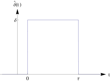
Figure 1: Rectangular shaped pulse in the phase $\delta(t)$.

II.2 Luttinger liquid: tunneling spectroscopy

The tunneling spectroscopy technique allows one to explore experimentally Keldysh Green functions of an interacting system that carry information about both tunneling density of states and energy distribution. Recent experiments on carbon nanotubes and quantum Hall edges have proved the efficiency of this technique in the context of 1D systemstunnel-spectroscopy ; tunnel-spectroscopy-qhe . The technological and experimental advances motivate the theoretical interest in the tunneling spectroscopy of strongly correlated 1D structures away from equilibrium GGM_long2010 ; jakobs08 ; gutman08 ; trushin08 ; pugnetti09 ; Ngo ; takei10 ; bena10 .

In the case of a LL formed by 1D interacting fermions, the Keldysh Green function may be evaluated theoretically via the non-equilibrium bosonization technique. Assuming that a long LL conductor is adiabatically coupled to two reservoirs (modeled as non-interacting 1D wiresMaslov ; Safi ; Ponomarenko ) with distribution functions $n_{R}(\epsilon)$ and $n_{L}(\epsilon)$ respectively, one obtains for the Green functions of the right movers GGM_long2010

$$G^{\gtrless}_{R}(\tau)=\mp\frac{i\Lambda}{2\pi u}\frac{\overline{\Delta}_{R\tau}[\delta_{R}]\overline{\Delta}_{L\tau}[\delta_{L}]}{(1\pm i\Lambda\tau)^{1+\gamma}}\,,$$ (4)

where $u=v/K$ is the sound velocity,

$$\gamma=(1-K)^{2}/2K\,,$$ (5)

and

$$K=(1+g/\pi v)^{-1/2}$$ (6)

is the standard LL parameter in the interacting region. The determinants $\overline{\Delta}_{\eta\tau}[\delta_{\eta}]$ ($\eta=R,L$) are given by Eq. (2) with $n(\epsilon)$ replaced by the corresponding distribution functions $n_{\eta}(\epsilon)$ and

$$\delta=\delta_{\eta}=\pi\frac{1+\eta K}{\sqrt{K}}\,.$$ (7)

The connection of the Luttinger liquid Green functions to Fredholm determinants is summarized in the last two rows of Table 1.

It is worth emphasizing that the the rectangular shape (3) of the pulse with the amplitude (7) is valid in the case when the coupling to reservoirs is smooth on the scale of the plasmon wave length $v/T$, $u/T$. In the opposite regime the pulse $\delta(t)$ entering (4) is fractionalized in a sequence of rectangular pulses GGM_long2010 . In the long-wire limit the corresponding determinant splits into a product of single-pulse (i.e Toeplitz-type) determinants. For definiteness, we focus on the adiabatic case in this paper.

	$\delta_{R}$	$\delta_{L}$	$\gamma$
$G_{\rm FES}^{>}(\tau)$	$2(\pi-\delta_{0})$	$0$	$\frac{\delta_{0}^{2}}{\pi^{2}}-\frac{2\delta_{0}}{\pi}$
$G_{R}^{>}(\tau)$	$2\pi\frac{1+K}{2\sqrt{K}}$	$2\pi\frac{1-K}{2\sqrt{K}}$	$\frac{(1-K)^{2}}{2K}$
$G_{L}^{>}(\tau)$	$2\pi\frac{1-K}{2\sqrt{K}}$	$2\pi\frac{1+K}{2\sqrt{K}}$	$\frac{(1-K)^{2}}{2K}$

Table 1: Non-equilibrium correlation functions of many-body problems: Fermi edge singularity ($G^{>}_{\rm FES}(\tau)$), Green functions of right- and left-moving fermions in a LL ($G^{>}_{\rm R}(\tau)$ and $G^{>}_{\rm L}(\tau)$). Evaluation of these correlation functions yields the results in the form of Fredholm-Toeplitz determinants $\tau^{-\gamma-1}\overline{\Delta}_{R}[\delta_{R}]\overline{\Delta}_{L}[\delta_{L}]$. The corresponding phases $\delta_{R,L}$ are presented in the second and third columns. (For LL an adiabatic coupling to reservoirs on the scale of the characteristic plasmon wave length is assumed.) The determinants are normalized to their values at zero temperature. The exponent $\gamma$ governing the zero-temperature correlation function is shown in the last column.

II.3 Ultraviolet regularization and reduction to Toeplitz matrix

Due to characteristic rectangular shape (3) of the pulses $\delta(t)$ the Fredholm determinants $\Delta_{\tau}(\delta)$ are in fact of the Toeplitz form. Specifically, one can write

$$\Delta_{\tau}[\delta]=\det[1+\hat{P}(e^{-i\delta}-1)\hat{n}\hat{P}]\,\,.$$ (8)

Here we have defined the projection operator

$$\hat{P}y(t)=\left\{\begin{array}[]{l}y(t)\,,\,\,\,{\rm for}\,\,\,t\in[0,\tau]\\ \\ 0\,,\,\,\,\,\,\,\,\,\,\,\,{\rm otherwise}\,.\end{array}\right.$$ (12)

The form (8) is convenient for peforming the ultraviolet regularization of the determinant $\Delta_{\tau}[\delta]$. Specifically, we discretize the time $t$ by introducing an elementary time step $\Delta t=\pi/\Lambda$, such that $t_{j}=j\Delta t$. This corresponds to restricting the energy variable $\epsilon$ to the range $[-\Lambda,\Lambda]$. We arrive then at a finite-dimensional determinant

$$\Delta_{N}[\delta]=\det[f(t_{j}-t_{k})]\,,\,\,\,0\leq j,k\leq N-1\,.$$ (13)

Here $N=\tau\Lambda/\pi$ and $f(t_{j}-t_{k})$ is Fourier transform of the function

$$f(\epsilon)=1+n(\epsilon)(e^{-i\delta}-1)\,.$$ (14)

The matrix elements $f(t_{j}-t_{k})$ depend on $j$ and $k$ via the difference $j-k$ only, so that the obtained matrix is of Toeplitz type.

In order to bring Eqs. (13), (14) to the canonical form used in the theory of Toeplitz matrices, we have to define the function $f(\epsilon)$ on the unit circle $|z|=1$. This is easily done by identifying the polar angle $\theta\in[-\pi,\pi]$ parametrizing the unit circle via $z=e^{i\theta}$ with the appropriately rescaled energy: $\theta=\pi\epsilon/\Lambda$. However, if this is done directly with the function (14), a non-physical jump will arise at $\theta=\pm\pi$. In order to eliminate it, one has to introduce an additional phase factor into the definition of $f(\epsilon)$:

$$f(\epsilon)=[1+n(\epsilon)(e^{-i\delta}-1)]e^{-i{\delta\over 2}{\epsilon\over\Lambda}}\,.$$ (15)

After the mapping to the unit circle, $z=e^{i\pi\epsilon/\Lambda}$, this defines a function $f(z)$ (known as the symbol of the Toeplitz matrix) that is perfectly smooth at $z=-1$. It will, however, have discontinuities (“Fisher-Hartwig singularities”) at the positions $z=e^{i\pi\epsilon_{j}/\Lambda}$ if the distribution function $n(\epsilon)$ has such discontinuities (“Fermi edges”) at $\epsilon_{j}$. We will be interested in the situation when there are several (at least two) such discontinuities.

It is worth emphasizing that the regularization (13), (15) makes explicit the dependence of the determinant $\Delta_{\tau}(\delta)$ on the integer part of $\delta/2\pi$ (thus making redundant the procedure of analytical continuation from $\delta\in[-\pi,\pi]$ to larger $|\delta|$ discussed in Ref. GGM_long2010, ). This allows us to directly compute the determinant at arbitrarily large (by absolute value) $\delta$.

As the matrix $\{f(t_{j}-t_{k})\}$ with $0\leq j,k\leq N-1$ is of Toeplitz form, results concerning the large-$N$ asymptotic behavior of Toeplitz determinats $\Delta_{N}$ can be applied. We summarize them in the next section. Physically, the large-$N$ limit corresponds to the regime of long time $\tau$, i.e. to infrared asymptotics of correlation functions under interest. (In the energy representation, this translates into low-energy behavior around singularities.)

Furthermore, Eqs. (13), (15) are also very convenient for numerical evaluation of the determinant $\Delta_{\tau}(\delta)$, providing us access to the full time (or, after Fourier transformation, energy) dependence of the correlation functions.

III Asymptotic properties of Toeplitz determinants

Toeplitz matrices and operators were introduced by O. Toeplitz a century ago. Since this time, asymptotic properties of Toeplitz determinants have been in a focus of interest of mathematicians, starting from the 1915 paper szego15 that was the first research paper by G. Szegö. The Szegö theorems szego39 valid for a smooth symbol yield the large-$N$ asymptotics of the determinant, which is exponential in $N$, with an $N$-independent prefactor. As was realized by Fisher and Hartwig fisher-hartwig , in the case of a symbol with singularities, the asymptotics acquires, in addition to the exponential factor, also a power-law factor. Thus, the infrared behavior of the Toeplitz determinant (13) includes non-trivial power-law factors if the function $f(z)$ is not smooth on the unit circle. The simplest example is the zero-temperature determinant Gutman10

$$\Delta_{N}[\delta,T=0]=e^{-i\delta N/2}\left(\frac{\pi}{\Lambda\tau}\right)^{\left(\frac{\delta}{2\pi}\right)^{2}}\\ \times G\left(1-\frac{\delta}{2\pi}\right)G\left(1+\frac{\delta}{2\pi}\right)\,$$ (16)

that has a power-law dependence on time in the long-time limit ($\Lambda\tau\gg 1)$.

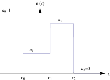
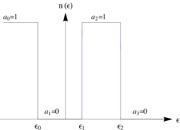
Figure 2: Left panel. Triple-step distribution: an example of multi-step distribution (17). Right panel. Simplest non-trivial distribution of the type (17) with identically zero dephasing.

Let us now consider a distribution function with multiple steps: (cf. Fig. 2):

$$n(\epsilon)=\left\{\begin{array}[]{ll}1\equiv a_{0}\,,&\qquad\epsilon<\epsilon_{0}\\ a_{1}\,,&\qquad\epsilon_{0}<\epsilon<\epsilon_{1}\\ \ldots&\\ a_{m}\,,&\qquad\epsilon_{m-1}<\epsilon<\epsilon_{m}\\ 0\equiv a_{m+1}\,,&\qquad\epsilon_{m}<\epsilon\,,\end{array}\right.$$ (17)

where $0\leq a_{j}\leq 1$, for $j=0,\dots,m$, We are interested in the Toeplitz determinant (13) for the multi-step distribution function (17). Let us split the phase $\delta$ as $\delta=2\pi M+\delta^{\prime}$, where $M$ is integer and $|\delta^{\prime}|<\pi$. We find it convenient to normalize the determinat by its zero-temperature value (16); the normalized determinant will be denoted as $\overline{\Delta}_{\tau}(\delta)$. According to the extended Fisher-Hartwig conjecture Gutman10 , it has the following long time asymptotics

$$\overline{\Delta}_{\tau}(\delta) = \frac{\exp\left[-i\tau\mu^{\prime}-\tau/2\tau_{\phi}\right]}{G(1-\delta/2\pi)G(1+\delta/2\pi)}$$ (18)

$$\times \sum_{n_{0}+\ldots+n_{m}=-M}e^{i\tau\sum_{j}n_{j}\epsilon_{j}}\left.\prod_{j<k}\left(\frac{1}{\tau U_{jk}}\right)^{-2\beta_{j}\beta_{k}}\prod_{j}G(1+\beta_{j})G(1-\beta_{j})\right|_{\beta_{j}=\beta^{\prime}_{j}+n_{j}}\,(1+\ldots).$$

Here we use the following notations: the exponents $\beta_{j}^{\prime}$ (satisfying $|{\rm Re}\beta_{j}^{\prime}|<1/2$) are

$$\beta_{i}^{\prime}={i\over 2\pi}\left[\ln(1-a_{i+1}+a_{i+1}e^{-i\delta})-\ln(1-a_{i}+a_{i}e^{-i\delta})\right],$$ (19)

the dephasing rate reads

$${1\over\tau_{\phi}}=2{\rm Im}\sum_{j}\beta_{j}^{\prime}\epsilon_{j}\,,$$ (20)

$G(x)$ is the Barnes G-function, $U_{jk}=|\epsilon_{j}-\epsilon_{k}|$, and $\mu^{\prime}=-{\rm Re}\sum_{j}\beta^{\prime}_{j}\epsilon_{j}$. Note that the ultraviolet regularization $\Lambda$ does not enter the normalized determinant. The asymptotic (18) is valid provided that $\tau U_{jk}\gg 1$ for all $j\neq k$. The summation goes over all sets of integer $n_{0},\ldots,n_{m}$ satisfying $n_{0}+\ldots+n_{m}=-M$; each such set yields the corresponding oscillatory exponent $e^{i\tau\sum_{j}n_{j}\epsilon_{j}}$. Equation (18) presents explicitly the leading asymptotic behavior for the factor multiplying each of these exponents. Apart from this dominant term, there will be in general also subleading (in powers of $1/t$) terms corresponding to the same exponent; these are abbreviated by $+\ldots$ in the last bracket.

The asymptotics (18) has a long history. The form of its leading term (the one with the slowest decay in $\tau$, i.e. with the smallest exponent $\alpha(n_{0}\,,\ldots n_{m})=2\mathop{\rm Re}\left[\sum_{j>k}\beta_{j}\beta_{k}\right]$) was suggested back in 1968 by Fisher and Hartwig fisher-hartwig . Since then, significant efforts were invested into the exact formulation, the proof, and extensions of the Fisher-Hartwig conjecture. For the case when a unique combination of integers $n_{i}$ exists that minimizes the exponent $\alpha(n_{0}\,,\ldots n_{m})$, the leading asymptotic term (including the corresponding numerical coefficient indicated in (18)) was rigorously derived by EhrhardtEhrhardt . In a recent seminal paper deift09 the theorem due to Ehrhardt was generalized for the case when there are several distinct sets of integers $\{n_{i}\}$ sharing the same minimal value of the exponent $\alpha(n_{0}\,,\ldots n_{m})$. It was proven that the leading term of the asymptotic expansion of the determinant $\Delta_{\tau}[\delta]$ at large $\tau$ is given by (18) where the sum should be restricted to the sets $\{n_{i}\}$ minimizing the exponent $\alpha(n_{0}\,,\ldots n_{m})$.

More recently, two of us and Gefen Gutman10 formulated and extended version of the Fisher-Hartwig conjecture [as shown in Eq. (18)] that includes a sum over all sets $\{n_{i}\}$ (which correspond to different branches of the logarithms) and captures the leading term of the expansion at every oscillation frequency $\sum_{j}n_{j}\epsilon_{j}$. This extension is very natural from the point of view of continutiy, as, under change of parameters, the dominant branch (that determines the leading asymptotics given by Ref. deift09, ) may become subdominant. This is particularly transparent in the energy representation of our problem discussed below: different branches then correspond to singularities near different energies; clearly, such a singularity will persist even when its exponent will become subdominant with respect to a singularity at other energy. Furthermore, the summation over branches has a clear physical meaning: it corresponds to processes including transfer of one or several electrons between different Fermi edges Gutman10 .

To illustrate how Eq.  (18) works, let us consider a simple case of the determinant at the phase $\delta=4\pi$, which can be evaluated exactly by a “refermionization” procedure GGM_long2010 . We assume for definiteness that the distribution function is of double step form with jumps at $\epsilon_{0}$ and $\epsilon_{1}$. (Generalization to a distribution function with more than two jumps is straightforward.) The exact result reads

$$\overline{\Delta}_{\tau}[4\pi]=a_{1}(a_{1}-1)\left[(\epsilon_{1}-\epsilon_{0})^{2}\tau^{2}-2\right]e^{-i(\epsilon_{0}+\epsilon_{1})\tau}\\ +(1-a_{1})^{2}e^{-2i\epsilon_{0}\tau}+a_{1}^{2}e^{-2i\epsilon_{1}\tau}\,.$$ (21)

On the other hand, considering the expansion (18) one gets at $\delta\rightarrow 4\pi$

$$\beta_{0}^{\prime}=(a_{1}-1)\frac{\delta^{\prime}}{2\pi}$$ (22)

$$\beta_{1}^{\prime}=-a_{1}\frac{\delta^{\prime}}{2\pi}$$ (23)

with $\delta^{\prime}\rightarrow 0$. Observing now that $G(x)$ has $k$-th order zero at $x=-k+1$ for any positive integer $k$ we conclude that at $\delta=4\pi$ (or generally for any $\delta$ being integer multiple of $2\pi$) the sum in (18) becomes finite. In the present case only the terms with $(n_{0}\,,\,n_{1})=(-1,-1)$, $(-2,0)$ and $(0,-2)$ contribute, yielding

$$\overline{\Delta}_{\tau}(4\pi)\simeq a_{1}(a_{1}-1)(\epsilon_{1}-\epsilon_{0})^{2}\tau^{2}e^{-i(\epsilon_{0}+\epsilon_{1})\tau}\\ +(1-a_{1})^{2}e^{-2i\epsilon_{0}\tau}+a_{1}^{2}e^{-2i\epsilon_{1}\tau}\,.$$ (24)

Comparing this asymptotic formula to the exact result (21), we see that Eq. (24) indeed perfectly reproduce leading factors for each oscillation frequency. The only term missing in Eq. (24) is

$$-2a_{1}(a_{1}-1)e^{-i(\epsilon_{0}+\epsilon_{1})\tau}\,,$$ (25)

which represents a small correction (due to an additional factor $\propto\tau^{-2}$) to the leading term at the same frequency $\epsilon_{0}+\epsilon_{1}$,

$$a_{1}(a_{1}-1)(\epsilon_{1}-\epsilon_{0})^{2}\tau^{2}e^{-i(\epsilon_{0}+\epsilon_{1})\tau}\,.$$ (26)

Such terms representing small power-law corrections to the leading contribution at the same frequency are indicated in Eq. (18) by the symbol $+\ldots$.

Let us note that, while being small with respect to the leading term at the same frequency, these corrections are not necessarily small with respect to leading terms at other frequencies. In particular, in the considered example the correction term on the frequency $\epsilon_{0}+\epsilon_{1}$, Eq. (25) is of the same order as the terms oscillating with frequencies $2\epsilon_{0}$ and $2\epsilon_{1}$ that are taken into account by Eq.  (24).

Thus, Eq. (18) captures explicitly the leading term for each frequency. A mathematically rigorous proof of this generalized form of the Fisher-Hartwig conjecture remains to be developed. Also, one may hope that it is possible to generalize Eq.(18) further, accounting also for sub-leading contribution (indicated as $+\ldots$ in Eq. (18)). A construction of such a full asymptotic expansion of the Toeplitz determinant was discussed very recently in Ref. Ivanov2011, for the special case $f(\epsilon)=1+(e^{-i\delta}-1)\Theta\left(U-|\epsilon|\right)$, where $\Theta(x)$ is the Heaviside theta function.

It is worth mentioning that for $\delta=2\pi$ Eq. (18) reproduces the exact result

$$\overline{\Delta}_{\tau}(2\pi)=(1-a)e^{-i\epsilon_{0}\tau}+ae^{-i\epsilon_{1}\tau}$$ (27)

without any corrections at all. While Eq. (27) is written for a double-step distribution, this statement is valid for any multi-step distribution as well. The only non-zero terms in Eq. (18) for $\delta=2\pi$ are those with all $n_{j}$ being equal to zero except for one equal to $-1$. The determinant demonstrates oscillations at frequencies $\epsilon_{j}$. All corrections of the type $+\ldots$ in Eq. (18) vanish. This implies that for values of $\delta\simeq 2\pi$ the correction terms $+\ldots$ in Eq. (18) have additional smallness.

Having clarified the status of the expansion (18), let us now discuss its implications. In a generic case, the power-law decay of $\overline{\Delta}_{\tau}(\delta)$ is cut off by the non-equilibrium dephasing time $\tau_{\phi}$ given by Eq. (20). Quite remarkably, the dephasing time is an oscillating function of the phase $\delta$ which translates, e.g., into the non-monotonous dependence of $\tau_{\phi}$ on the interaction strength in Luttinger liquid GGM_long2010 . The dephasing is absent when $\delta^{\prime}=0$ in which case $\Delta_{\tau}(\delta)$ can be represented in terms of a free fermionic theory.

Dephasing is also absent for the case when all $a_{j}=0,\,1$. This corresponds to the case of a pure electronic state (i.e. characterized by a wave function rather than by a density matrix). The simplest non-trivial distribution of the type Eq. (17) that has this property is the triple-step distribution of Fig. 2 (right panel). We stress that in this “ideal inverse population” case the dephasing rate is identically equal to zero, regardless of the value of the phase $\delta$. Apart from being interesting on a pure theoretical grounds, the distributions realizing the inverse population of electronic states are also expected to be experimentally relevant, as they are inevitably generated in course of evolution of a smooth perturbation of electronic density if the spectral curvature is taken into account Wiegmann .

The power-law decay of $\overline{\Delta}_{\tau}(\delta)$ in the time domain is translated into the singular energy dependence of correlation functions in energy representation. Specifically, every term in the expansion (18) gives rise to a singular contribution

$$\mathop{\rm Re}\left[e^{-i\frac{\pi}{2}(\gamma+1)}\frac{\prod_{j}G(1+\beta_{j})G(1-\beta_{j})}{G(1-\delta/2\pi)G(1+\delta/2\pi)}\Gamma\left(\gamma_{n_{0}\ldots n_{m}}\right)\prod_{j<k}\left(\frac{1}{U_{jk}}\right)^{-2\beta_{j}\beta_{k}}\frac{1}{\left(i\epsilon+i\sum_{j}n_{j}\epsilon_{j}-i\mu^{\prime}-\tau/2\tau_{\phi}\right)^{\gamma_{n_{0}\ldots n_{m}}}}\right]$$ (28)

to the Fourier transform of $\overline{\Delta}_{\tau}[\delta]/(i\tau)^{\gamma+1}$ with the exponent

$$\gamma_{n_{0}\ldots n_{m}}=\gamma-\left.2\sum_{j<k}\beta_{j}\beta_{k}\right|_{\beta_{j}=\beta_{j}^{\prime}+n_{j}}\,.$$ (29)

In Sec. IV we will compare Eqs. (28), (29) with the results of numerical evaluation of Toeplitz determinants.

IV Numerical analysis

In this Section, we present results of the numerical analysis of the Toeplitz determinants (13) which allows us to evaluate the many-body Green functions in the whole range of times (energies). We will further demonstrate that the numerics gives full support to the asymptotic expansion (28), (29).

IV.1 Numerical procedure

To be specific, we will consider fermions with the following two types of many-step distributions: (i) double-step distribution

$$n_{d}(\epsilon)=\left\{\begin{array}[]{ll}1\equiv a_{0}\,,&\qquad\epsilon<\epsilon_{0}=-U/3\\ a_{1}=1/3\,,&\qquad\epsilon_{0}<\epsilon<\epsilon_{1}=2U/3\\ 0\equiv a_{2}\,,&\qquad\epsilon_{1}<\epsilon\,,\end{array}\right.$$ (30)

and (ii) triple-step distribution with the “maximal” inverse population (Fig. 2, right panel)

$$n_{t}(\epsilon)=\left\{\begin{array}[]{ll}1\equiv a_{0}\,,&\qquad\epsilon<\epsilon_{0}=-3U/4\\ a_{1}=0\,,&\qquad\epsilon_{0}<\epsilon<\epsilon_{1}=-U/2\\ a_{2}=1\,,&\qquad\epsilon_{1}<\epsilon<\epsilon_{2}=U/4\\ 0\equiv a_{3}\,,&\qquad\epsilon_{2}<\epsilon\,.\end{array}\right.$$ (31)

In these equations we have expressed all the energies $\epsilon_{k}$ in terms of characteristic scale $U=\epsilon_{m}-\epsilon_{0}$ associated with the distribution function.

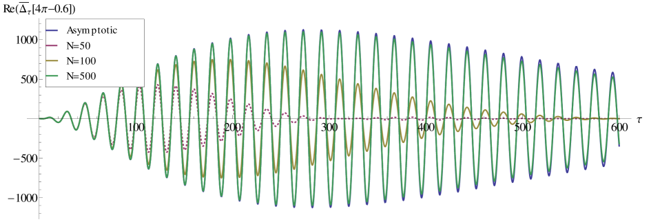
Figure 3: Time dependence of the determinant $\overline{\Delta}_{\tau}[4\pi-0.6]$. The distribution function was taken to be $n_{d}(\epsilon)$, Eq. (30). Numerical results for matrix sizes $N=50$, 100, and 500, as well the leading asymptotic term (34) are shown. The numerical result for $N=500$ is almost indistinguishable from the asymptotics.

Let us consider the normalized determinant $\overline{\Delta}_{\tau}[U,\delta]$ and its finite-dimensional approximation $\overline{\Delta}_{N}[U/\Lambda,\delta]$. Here we made explicit the dependence of the determinants on $U$. At $\tau$ and $U$ fixed, $\overline{\Delta}_{N}[U/\Lambda,\delta]$ has a finite limit as $\Lambda\rightarrow\infty$ which is a cutoff-independent function of the dimensionless variable $U\tau$ only:

$$\overline{\Delta}_{\tau}[U,\delta]\equiv\overline{\Delta}[U\tau,\delta] = \lim_{\Lambda\rightarrow\infty}\overline{\Delta}_{N=\frac{\tau\Lambda}{\pi}}\left[\frac{U\tau}{\pi N},\delta\right]$$ (32)

$$= \lim_{N\rightarrow\infty}\overline{\Delta}_{N}\left[\frac{U\tau}{\pi N},\delta\right]\,.$$ (33)

Equation (33) constitutes the starting point for our numerical analysis. With a simple Mathematica code we are able to go within a quite short computation time up to the size of the Toeplitz matrix $N=500$, which is typically sufficient for the convergence to the large-$N$ limit for relevant values of $U\tau$.

The convergence properties of our procedure become generally worse at large $\delta$. Thus, we chose to illustrate them with the calculation of the determinant at the phase $4\pi-0.6$ which is larger then any phase we will encounter in the next section. This choice also enables us to demonstrate clearly the presence of the correction terms indicated by $+\ldots$ in Eq. (18).

From now on, we measure $\tau$ in units of $1/U$. Figure 3 shows the result of numerical evaluation of the normalized Toeplitz determinant $\overline{\Delta}_{\tau}[4\pi-0.6]$ for the double-step distribution function $n_{d}$ given by Eq. (30). We have plotted the data for $N=50,100,500$ together with leading term of the asymptotic expansion (18), the one with $n_{0}=n_{1}=-1$

$$\overline{\Delta}_{\tau}^{A1}[4\pi-0.6]\approx(0.25+0.026i)e^{-i\tau(\epsilon_{1}+\epsilon_{0})-\tau/2\tau_{\phi}}\tau^{1.81}\,.$$ (34)

Here $\tau_{\phi}\approx 77$ and $\epsilon_{0}+\epsilon_{1}=1/3$. Note the fast convergence with the increase of the matrix size and perfect agreement with the predicted asymptotic behavior. We stress that the asymptotic fit used here has no adjustable parameters.

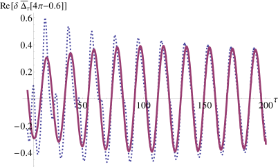
Figure 4: Difference between the numerically evaluated determinant (shown in Fig. 3) and the asymptotic approximation for $N=5000$. The electronic distribution was the double-step distribution $n_{d}(\epsilon)$. Dotted line: only the leading term (34) was subtracted; full line: three main harmonics (Fisher-Hartwig branches) of the expansion (18) have been taken into account. The remaining difference is due to a correction [of the type indicated by $+\ldots$ in Eq. (18)] to the leading harmonic (34).

Let us now explore the effect of the other terms in the expansion (18). The next two terms are characterized by $(n_{0},n_{1})=(-2,0)$ and $(n_{0},n_{1})=(0,-2)$. Apart from the exponential damping at scales larger then $\tau_{\phi}$ they decay as $\tau^{-0.12}$ and $\tau^{-0.25}$ respectively. Since in this case powers of the leading and the subleading harmonics are substantially different, a reliable observation of the subleading ones requires more substantial numerical efforts. To achieve the required accuracy, we use larger values of the matrix size ($N=5000$). Note that in Sec. IV.1, IV.3, where we focus on smaller values of the phase shift $\delta$, subleading harmonics will be much more pronounced and easily seen.

The difference between the numerically calculated Toeplitz determinant (13) and its asymptotic approximation 18) is shown in Fig. 4. The dotted line corresponds to the difference between the numerical result and the leading term (34). The solid line is the difference between the numerical result and the first three terms in the expansion (18). As expected, inclusion of the terms $(n_{0},n_{1})=(-2,0)$ and $(n_{0},n_{1})=(0,-2)$ improves the agreement between the asymptotics and the exact results. Indeed, the oscillations at high frequencies, that are clearly seen on a dotted line, are absent on the solid line. Nevertheless, a clear difference between the exact result and the asymptotic formula remains, which is predominantly due to the correction [of the type $+\ldots$ in Eq. (18)] to the leading (oscillating with frequency $\epsilon_{1}+\epsilon_{2}=1/3$) harmonic.

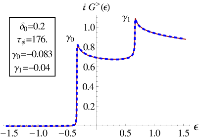
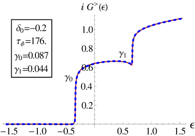
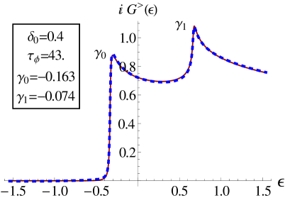
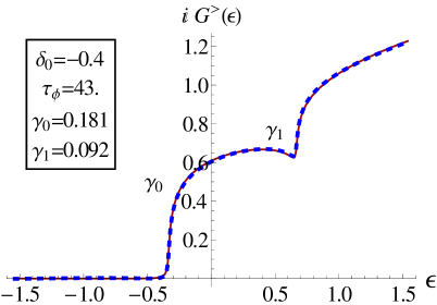
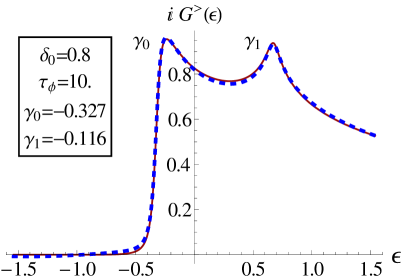
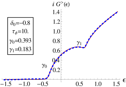
Figure 5: X-ray absorption spectra at different values of the scattering phase $\delta_{0}$ for the double-step distribution function of electrons $n_{d}(\epsilon)$ specified in Eq. (30). The solid lines represent the result of numerical evaluation of Toeplitz determinants while the dotted lines show the fits based on the asymptotics (18, 28). The legend shows the corresponding dephasing time $\tau_{\phi}$ together with the exponents $\gamma_{0}$ and $\gamma_{1}$ governing the singular behavior of $G^{>}(\epsilon)$ at $\epsilon=\epsilon_{0}=-1/3$ and $\epsilon=\epsilon_{1}=2/3$.

We have thus demonstrated that, even for a relatively large phase $\delta$, the numerical simulations work perfectly and that the large-$t$ behavior is fully understood in the framework of the asymptotic expansion. In the sequel, we will present the results for two physical problems of our interest (FES and Luttinger liquid) in the energy domain. This is more natural physically (as this corresponds to spectroscopy measurements) and also gives us the possibility to separate the contributions of different harmonics in (18) within the same graph. We note that the Green functions $G^{\gtrless}(\tau)$ are obtained from a Toeplitz determinant (or a product of two Toeplitz determinants) by multiplication with $1/(\Lambda\tau)^{\gamma+1}$ (with $\gamma$ being the zero temperature exponent, see the last column of Table 1). Thus,

$$G^{\gtrless}(\epsilon)=\left(\frac{U}{\Lambda}\right)^{\gamma}\widetilde{G}^{\gtrless}(\epsilon/U)\,,$$ (35)

where the functions $\widetilde{G}^{\gtrless}(\epsilon/U)$ are cutoff independent. From now on we omit the energy independent factor $\left(U/\Lambda\right)^{\gamma}$ from the Green functions and measure all the energies in units of the characteristic scale $U$.

IV.2 Fermi edge singularity

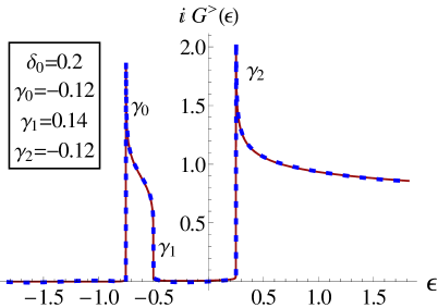
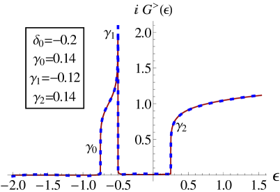
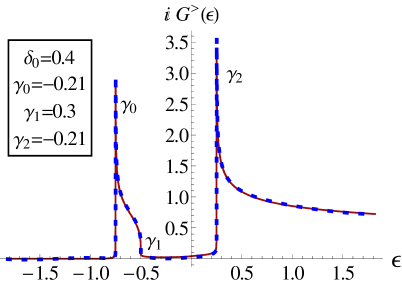
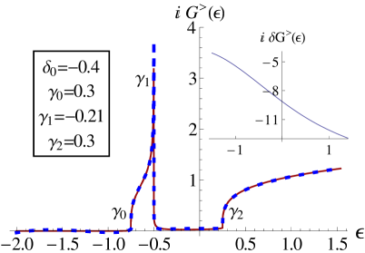
Figure 6: X-ray absorption spectra of the non-equilibrium FES problem with triple-step distribution of the electrons $n_{t}(\epsilon)$ (see. Eq. (31)) at relatively small scattering phase $\delta_{0}=\pm 0.2,\>\pm 0.4,\>\pm 0.8$. The solid lines represent the result of numerical evaluation of Toeplitz determinants while the dots show the fits based on the asymptotic expansion (18). For the chosen distribution function the dephasing rate $1/\tau_{\phi}$ is identically zero and the singularities are not smeared. The last graph in the second column has an inset exemplifying the smooth function $\delta G^{>}(\epsilon)$ added to the asymptotic expression to fit the numerical data.

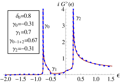
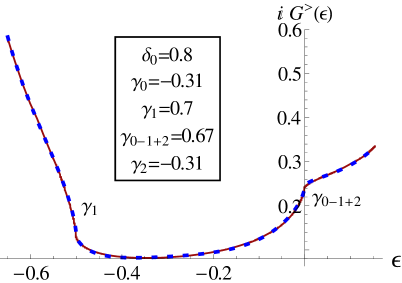
Figure 7: X-ray absorption spectra in the non-equilibrium FES problem with triple-step distribution of the electrons. The electronic distribution was the same as on Fig. 6 but the phase $\delta_{0}$ is now larger. In addition to singularities at Fermi edge $\epsilon_{k}$ one observes now a singularity at energy $\epsilon_{0}-\epsilon_{1}+\epsilon_{2}=0$ with the exponent $\gamma_{0-1+2}$ originating from the term with $n_{0}=-1\,,\,n_{1}=1\,,\,n_{2}=-1$ in the sum (18).

According to Eq. (1), the emission/absorption rates out of equilibrium are given by a single Toeplitz determinant. We analyze the case of a double-step distribution function $n_{d}(\epsilon)$, Eq. (30), first. The results for the different values of the scattering phase $\delta_{0}$ are shown in Fig. 5.

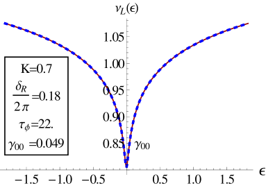
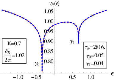
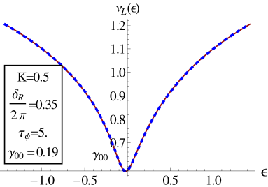
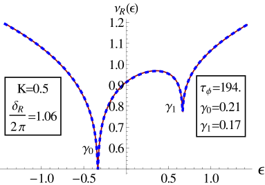
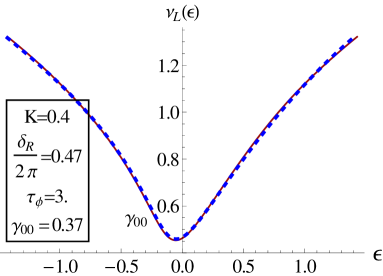
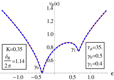
Figure 8: TDOS $\nu_{\eta}(\epsilon)$ of left (first column) and right (second column) particles in a non-equilibrium Luttinger liquid. The incoming right movers have the double-step distribution $n_{d}(\epsilon)$. The incoming left movers are assumed to have zero temperature, so that $\overline{\Delta}_{L\tau}[\delta_{L}]\equiv 1$. The phase $\delta_{R}$ entering the nontrivial determinant $\overline{\Delta}_{R}[\delta_{R}]$ is in the vicnitiy of $0$ for the case of $\nu_{L}(\epsilon)$ and in the vicinity of $2\pi$ in the case of $\nu_{R}(\epsilon)$, as indicated in the legend.

The solid lines in Fig. 5 represent the result of numerical evaluation of Toeplitz determinants, while the dotted lines show the fits based on the asymptotic formulas (18), (28). Only the dominant terms in the sum (18) were retained (the terms with $n_{0}=-1$, $n_{1}=0$ or vice versa). Using the expansion (18), we are able to calculate the singular behavior of $G^{>}(\epsilon)$. The regular part is controlled by the behavior of $G^{>}(\tau)$ at small $\tau$ and therefore contains the information that is not retained when one uses the asymptotic expressions. In order to compare the singular behavior predicted by the asymptotic formulas (18), (28) with the exact results, we add a smooth function $\delta G^{>}(\epsilon)$ to the Eqs. (18), (28). We choose $\delta G^{>}(\epsilon)$ in the form of a polynomial of a relatively low order with coefficients that are adjusted to optimize the fit. In fact, already a second polynomial is sufficient to get a rather good fit, and we used it in most of the cases. In several cases we used a fourth order poynomial. An example of such a smooth function $\delta G^{>}(\epsilon)$ is shown in Fig. 6 (see inset of the lower right graph).

In agreement with the analytical predictions, the absorption spectra shown in Fig. 5 demonstrate singular behavior $G^{>}_{FES}(\epsilon)\sim\left(\epsilon-\epsilon_{k}+\frac{2i}{\tau_{\phi}}\right)^{\gamma_{k}}$ near the Fermi edges $\epsilon_{k}\,,\,k=0,1$. Note that the exponents at two edges are different, which is a very good demonstration of the importance of summation over all Fisher-Hartwig branches in Eqs. (18), (28). One observes the enhancement of absorption near the Fermi edges the for $\delta_{0}>0$. Contrary, for $\delta_{0}<0$ the absorption is suppressed. Upon increase of the modulus of the scattering phase $\delta_{0}$, the exponents $\gamma_{k}$ and the inverse dephasing time $\tau_{\phi}^{-1}$ grow by absolute value. Simultaneously, the dephasing increases, which induces a stronger smearing of singularities.

In Fig. 6 we plot the results for triple-step distribution, $n_{t}(\epsilon)$, and for relatively small values of the scattering phase $\delta_{0}$. At chosen $\delta_{0}$ the dominant terms in the expansion (18) are those with all $n_{i}=0$ except for one $n_{k}=-1$ and the only visible singularities are located at the Fermi edges $\epsilon_{k}$. In contrast to the case of double-step distribution, the growth of the scattering phase $\delta_{0}$ is not accompanied by smearing of the singularities, since the dephasing rate $1/\tau_{\phi}$ is identically zero.

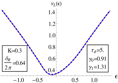
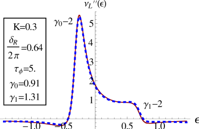
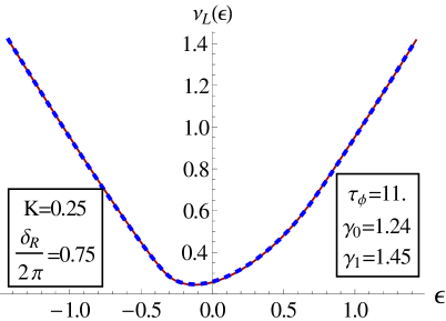
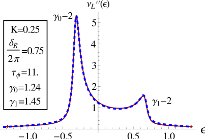
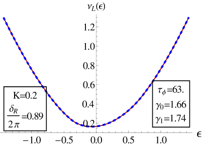
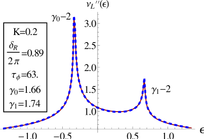
Figure 9: Non-monotonous dependence of the non-equilibrium dephasing in a Luttinger liquid on the interactions strength. The incoming right movers have double-step distribution $n_{d}(\epsilon)$. The incoming left movers are assumed to have zero temperature. The interaction is now sufficiently strong so that the phase $\delta_{R}$ governing the density of states for the left movers is close to $2\pi$. Correspondingly, the dominant singularities in $\nu_{L}(\epsilon)$ are now located at $\epsilon_{1}$ and $\epsilon_{2}$. The exponents $\gamma_{0}$ and $\gamma_{1}$ are positive and large and the singular behavior of $\nu_{L}(\epsilon)$ is difficult to see directly (left panels). It becomes evident, however, if one considers the second derivative of TDOS, $\nu_{L}^{\prime\prime}(\epsilon)$ (right panels).

As $\delta=2\pi-2\delta_{0}$ deviates further from $2\pi$, additional terms in the series (18) become important, as illustrated in Fig. 7. In particular, at $\delta_{0}=0.8$, apart from the singularities at Fermi edges $\epsilon_{k}$ a new one (at $\epsilon=\epsilon_{0}-\epsilon_{1}+\epsilon_{2}=0$) with the exponent $\gamma_{0-1+2}$ is clearly seen. It originates from the term $n_{0}=-1\,,\,n_{1}=1\,,\,n_{2}=-1$ in Eq. (18). This once more confirms the extended Fisher-Hartwig conjecture (18) with the summation over all branches.

IV.3 Tunneling into non-equilibrium Luttinger liquid

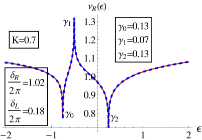
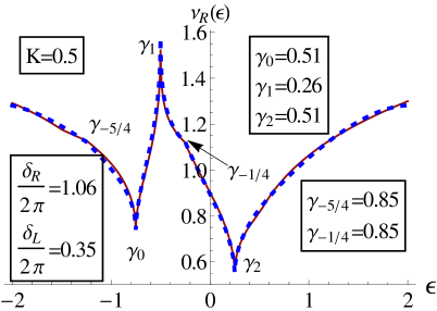
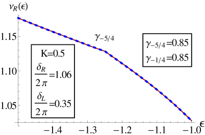
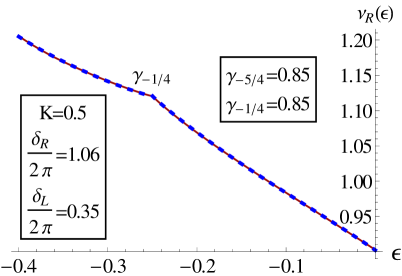
Figure 10: The density of states in the Luttinger liquid coupled to two reservoirs with the triple-step distribution $n_{t}(\epsilon)$. There is no dephasing, so that the singularities are sharp. At weak interaction ($K=0.7$, upper right plot), the most important terms in the right determinant $\overline{\Delta}_{R\tau}[\delta_{R}]$ oscillate as a function of time $\tau$ with frequencies $\epsilon_{k}$, $k=0\,,\,1\,,\,2$. On the other hand, the leading contribution to the left determinant decays without oscillations, and the oscillatory terms are very small (decay with much larger exponents). This leads to the singular behavior of the density of states at $\epsilon_{k}$. As the Luttinger parameter decreases ($K=0.5$, upper left plot), the subleading oscillating terms in $\overline{\Delta}_{L\tau}[\delta_{L}]$ come into play. This leads to additional (weak) singularities in $\nu_{R}(\epsilon)$ at $\epsilon=-5/4$ and $\epsilon=-1/4$. The corresponding regions of energy are magnified in the lower plots.

Let us now turn to another application of Toeplitz determinants, the tunneling into the Luttinger liquid. We begin by considering the simplest case, when the incoming right-moving electrons have the double-step distribution function $n_{d}(\epsilon)$, while the left movers are held at zero temperature. In this case the determinant $\overline{\Delta}_{L\tau}[\delta_{L}]$ in Eq. (4) is identically equal to unity. If the interaction is not too strong and one is interested in the density of states for the left-movers, the phase $\delta_{R}$ entering the non-trivial determinant $\overline{\Delta}_{R\tau}[\delta_{R}]$ is close to zero. On the other hand, the correlation functions of the right-movers are given by the determinants at phase $\delta_{R}$ close to $2\pi$. Correspondingly, the dominant singularity in the density of states $\nu_{L}(\epsilon)$ for the left particles is the one at $\epsilon=0$ while main singularities of $\nu_{R}(\epsilon)$ are at $\epsilon=\epsilon_{0}\,,\,\epsilon_{1}$. This behavior is illustrated in Fig. 8. Note that the left-moving electrons are dephased much strongerGGM_long2010 than the right-moving.

The behavior of $\nu_{L}(\epsilon)$ at stronger interaction (see Fig. 9) demonstrates the non-monotonous dependence of the dephasing on the Luttinger liquid parameter $K$. For $K<(3-\sqrt{5})/2\approx 0.38$, the phase $\delta_{R}>\pi$, and the leading singularities in $\nu_{L}$ are those at $\epsilon_{0}$ and $\epsilon_{1}$. They can be clearly seen if one plots the second derivative of the density of states with respect to energy (Fig. 9, left panel). Note that the smearing of those singularities decreases (i.e. singularities sharpen) with increasing interaction strength $K=0.3\to 0.25\to 0.2$, as $K$ evolves towards $K=3-2\sqrt{2}\approx 0.17$, where $\delta_{R}=2\pi$ and the dephasing is absent.

Finally, we consider an interacting wire with triple-step distribution $n_{t}$ for both left and right moving electrons. In this case, both determinants in Eq. (4) are nontrivial. The corresponding density of states is shown in Fig. 10. At weak interaction ($K=0.7$, upper-left panel of Fig. 10), the right determinant $\overline{\Delta}_{R\tau}[\delta_{R}]$ oscillates as a function of time $\tau$ with frequencies $\epsilon_{k}$, $k=0\,,\,1\,,\,2$, while the left determinant decays mostly without oscillations, This leads to the singular behavior of the density of states at $\epsilon_{k}$. As the Luttinger parameter decreases ($K=0.5$, upper-right panel of Fig.10), sub-leading oscillating terms in $\overline{\Delta}_{L}\tau[\delta_{L}]$ come into play and additional (weak) singularities in $\nu_{R}(\epsilon)$ appear at $\epsilon=-5/4$ and $\epsilon=-1/4$.

V Summary and outlook

To summarize, we have explored single-particle Green functions were of many-body fermionic systems in non-equilibrium settings characterized by multiple-step energy distribution functions. By using a periodic ultraviolet regularization, the problem is reduced to that of Toeplitz determinants. We have carried out numerical calculation of the corresponding Toeplitz determinants and thus obtained the results for the non-equilibrium Green functions in the entire energy range. Further, by employing the extended Fisher-Hartwig conjecture, we have analytically determined the energy dependence of the Green functions near each of the Fermi edges.

The obtained Green functions show, in the energy representation, power-law singularities near multiple edges. The singularities are in general characterized by different power-law exponents and are smeared by dephasing processes. In the special case of a distribution function with population inversion that alternates between $n=1$ and $n=0$, the dephasing is absent (i.e. the singularities are sharp) and the TDOS (or the absorption rate) exhibits enhancement and suppression in alternating succession.

The results of the numerical and analytical methods perfectly agree, thus confirming the validity of the extended Fisher-Hartwig conjecture.

We close the paper by listing some of future research directions:

• It would be interesting to see whether an explicit form of correction terms within each harmonic [those abbreviated by $+\ldots$ in Eq.  (18)] can be found. Further, a rigorous mathematical proof of the extended Fisher-Hartwig conjecture would be certainly desirable.

• One can consider many-body correlation functions in the non-equilibrium setups discussed above. This problem can be reduced to determinants that are of a form more general than the Toeplitz one. Some results in this direction will be reported soon in-preparation .

• It would be important to further extend the Fisher-Hartwig conjecture in order to include Toeplitz matrices with matrix symbols.

VI Acknowledgments

This paper has been prepared for publication in a volume commemorating Yehoshua Levinson. Two of us were very fortunate to know Yehoshua personally, to attend his lecture courses, to collaborate with him, and to enjoy numerous physics discussions with him. We owe to him much of our understanding of non-equilibrium phenomena in condensed-matter physics.

We thank A.R. Its for illuminating discussions of the Fisher-Hartwig conjecture deift09 and its extended version Gutman10 . We also thank R. Berkovits for useful discussions and collaboration on an early stage of this work, and V.V. Cheianov and D.A. Ivanov for useful discussions. I.V.P. acknowledges financial support by Alexander von Humboldt foundation. Financial support by German-Israeli Foundation, Israeli Science Foundation, DFG Center for Functional Nanostructures, and Bundesministerium für Bildung und Forschung is gratefully acknowledged. A.D.M. thanks KITP UCSB for hospitality during the completion of this work.

References

- (1) P.W. Anderson, Phys. Rev. Lett. 18, 1049 (1967).
- (2) P. Nozières and C. T. De Dominicis, Phys. Rev. 178, 1097 (1969).
- (3) S. Tomonaga, Prog. Theor. Phys. 5, 544 (1950); J. M. Luttinger, J. Math. Phys. 4, 1154 (1963); D.C. Mattis and E.H. Lieb, J. Math. Phys. 6, 304 (1965).
- (4) A. Luther and I. Peschel, Phys. Rev. B 9, 2911 (1974).
- (5) J. Kondo, Prog. Theor. Phys. 32, 37 (1964).
- (6) G. Yuval and P. W. Anderson, Phys. Rev. B 1, 1522 (1970).
- (7) E.H. Lieb and Werner Liniger, Phys. Rev. 130 1605 (1963); E.H. Lieb, Phys. Rev. 130 (1963).
- (8) V.E. Korepin, N.M. Bogoliubov and A.G. Izergin, Quantum Inverse Scattering Method and Correlation Functions ( Cambridge University Press, 1993).
- (9) D.B. Gutman, Y. Gefen, and A.D. Mirlin, Europhys. Letters 90, 37003 (2010); Phys. Rev. B 81, 085436 (2010).
- (10) D.B. Gutman, Y. Gefen, and A.D. Mirlin, Phys. Rev. Lett. 105, 256802 (2010)
- (11) D.B. Gutman, Y. Gefen, and A.D. Mirlin, J. Phys. A: Math. Theor. 44 (2011) 165003
- (12) M. Stone, Bosonization (World Scientific, 1994).
- (13) J. von Delft and H. Schoeller, Annalen Phys. 7, 225 (1998).
- (14) A.O. Gogolin, A.A. Nersesyan, and A.M. Tsvelik, Bosonization in Strongly Correlated Systems, (University Press, Cambridge 1998).
- (15) T. Giamarchi, Quantum Physics in One Dimension, (Claverdon Press Oxford, 2004).
- (16) D.L. Maslov, in Nanophysics: Coherence and Transport, edited by H. Bouchiat, Y. Gefen, G. Montambaux, and J. Dalibard (Elsevier, 2005), p.1.
- (17) M.E. Fisher and R.E. Hartwig, Toeplitz determinants: some applications, theorems, and conjectures, in Advances in Chemical Physics: Stohastic processes in chemical physics, Volume 15, ed. by K.E. Schuler (John Wiley & Sons, 1969), p.333.
- (18) P. Deift, A. Its, and I. Krasovsky, Ann. Math. 174-2, 1243 (2011).
- (19) K.D. Schotte and U. Schotte, Phys. Rev. B 182, 479 (1969).
- (20) D.A. Abanin and L.S. Levitov, Phys. Rev. Lett. 93, 126802 (2004); D.A. Abanin and L.S. Levitov, Phys. Rev. Lett. 94, 186803 (2005).
- (21) Y.-F. Chen, T. Dirks, G. Al-Zoubi, N. Birge, and N. Mason Phys. Rev. Lett. 102, 036804 (2009).
- (22) C. Altimiras, H. le Sueur, U. Gennser, A. Cavanna, D. Mailly, F. Pierre, Nature Physics 6, 34 (2010).
- (23) S.G. Jakobs, V. Meden, and H. Schoeller, Phys. Rev. Lett. 99, 150603 (2007).
- (24) D. B. Gutman, Y. Gefen, and A. D. Mirlin Phys. Rev. Lett. 101, 126802 (2008); Phys. Rev. B 80, 045106 (2009).
- (25) M. Trushin and A. L. Chudnovskiy, Europhys. Letters, 82, 17008 (2008).
- (26) S. Pugnetti, F. Dolcini, D. Bercioux, and H. Grabert, Phys. Rev. B 79, 035121 (2009).
- (27) S. Ngo Dinh, D.A. Bagrets, and A.D. Mirlin, Phys. Rev. B 81, 081306 (R) (2010).
- (28) S. Takei, M. Milletarì, and B. Rosenow, Phys. Rev. B 82, 041306(R) (2010).
- (29) C. Bena, Phys. Rev. B 82, 035312 (2010).
- (30) D.L. Maslov and M. Stone, Phys. Rev. B 52, R5539 (1995).
- (31) I. Safi and H.J. Schulz, Phys. Rev. B 52, R17040 (1995).
- (32) V.V. Ponomarenko, Phys. Rev. B 52, R8666 (1995).
- (33) G. Szegö, Ein Grenzwertsatz über die Toeplitzschen Determinanten einer reellen positiven Funktion, Mathematische Annalen 76, 490 (1915).
- (34) G. Szegö, Orthogonal Polynomials, AMS Colloquium Publ. 23 (AMS, 1939).
- (35) T. Ehrhardt, Operator Theory: Adv. Appl. 124, 217 (2001)
- (36) A. G. Abanov, D. A. Ivanov, Y. Qian, J. Phys. A: Math. Theor. 44, 485001 (2011); D. A. Ivanov, A. G. Abanov, V. V. Cheianov, arXiv:1112.2530 (2011).
- (37) E. Bettelheim, A.G. Abanov, P. Wiegmann, Phys. Rev. Lett. 97, 246402 (2006).
- (38) I.V. Protopopov, D.B. Gutman, A.D. Mirlin, in preparation.