Barriers in Concurrent Separation Logic:
Now With Tool Support!

Abstract.

We develop and prove sound a concurrent separation logic for Pthreads-style barriers. Although Pthreads barriers are widely used in systems, and separation logic is widely used for verification, there has not been any effort to combine the two. Unlike locks and critical sections, Pthreads barriers enable simultaneous resource redistribution between multiple threads and are inherently stateful, leading to significant complications in the design of the logic and its soundness proof. We show how our logic can be applied to a specific example program in a modular way. Our proofs are machine-checked in Coq. We showcase a program verification toolset that automatically applies the logic rules and discharges the associated proof obligations.

1. Introduction

In a shared-memory concurrent program, threads communicate via a common memory. Programmers use synchronization mechanisms, such as critical sections and locks, to avoid data races. In a data race, threads “step on each others’ toes” by using the shared memory in an unsafe manner. Recently, concurrent separation logic has been used to formally reason about shared-memory programs that use critical sections and (first-class) locks [29, 22, 20, 21]. Programs verified with concurrent separation logic are provably data-race free.

What about shared-memory programs that use other kinds of synchronization mechanisms, such as semaphores? The general assumption is that other mechanisms can be implemented with locks, and that reasonable Hoare rules can be derived by verifying their implementation. Indeed, the first published example of concurrent separation logic was implementing semaphores using critical sections [29]. Unfortunately, not all synchronization mechanisms can be easily reduced to locks in a way that allows for a reasonable Hoare rule to be derived. In this paper we introduce a Hoare rule that natively handles one such synchronization mechanism, the Pthreads-style barrier.

Pthreads (POSIX Threads) is a widely-used API for concurrent programming, and includes various procedures for thread creation/destruction and synchronization [9]. When a thread issues a barrier call it waits until a specified number (typically all) of other threads have also issued a barrier call; at that point, all of the threads continue. Although barriers do not get much attention in theory-oriented literature, they are very common in numerical applications code. PARSEC is the standard benchmarking suite for multicore architectures, and has thirteen workloads selected to provide a realistic cross-section for how concurrency is used in practice today; a total of five (38%) of PARSEC’s workloads use barriers, covering the application domains of financial analysis (blackscholes), computer vision (bodytrack), engineering (canneal), animation (fluidanimate), and data mining (streamcluster) [5]. A common use for barriers is to manage large numbers of threads in a pipeline setting. For example, in a video-processing algorithm, each thread might read from some shared common area containing the most recently completed frame while writing to some private area that will contain some fraction of the next frame. (A thread might need to know what is happening in other areas of the previous frame to properly handle objects entering or exiting its part of the current frame.) In the next iteration, the old private areas become the new shared common area as the algorithm continues.

Our key insight is that a barrier is used to simultaneously redistribute ownership of resources (typically, permission to read/write memory cells) between multiple threads. In the video-processing example, each thread starts out with read-only access to the previous frame and write access to a portion of the current frame. At the barrier call, each thread gives up its write access to its portion of the (just-finished) frame, and receives back read-only access to the entire frame. Separation logic (when combined with fractional permissions [6, 15]) can elegantly model this kind of resource redistribution. Let $\mathit{Pre}_{i}$ be the preconditions that held upon entering the barrier, and $\mathit{Post}_{i}$ be the postconditions that will hold after being released; then the following equation is almost true:

$$\raisebox{-7.0pt}{$\stackrel{{\scriptstyle\mbox{\huge{{$\tt*$}}}}}{{{}_{i}}}$}~{}{\vspace{-10pt}\mathit{Pre}_{i}}\qquad=\qquad\raisebox{-7.0pt}{$\stackrel{{\scriptstyle\mbox{\huge{{$\tt*$}}}}}{{{}_{i}}}$}~{}{\vspace{-10pt}\mathit{Post}_{i}}$$ (1)

Pipelined algorithms often operate in stages. Since barriers are used to ensure that one computation has finished before the next can start, the barriers need to have stages as well—a piece of ghost state associated with the barrier. We model this by building a finite automaton into the barrier definition. We then need an assertion, written $\mathsf{barrier}(\mathit{bn},\pi,\mathit{cs})$, which says that barrier $\mathit{bn}$, owned with fractional permission $\pi$, is currently in state $\mathit{cs}$. The state of a barrier changes exactly as the threads are released from the barrier. We can correct equation (1) by noting that barrier $\mathit{bn}$ is transitioning from state $\mathit{cs}$ (current state) to state $\mathit{ns}$ (next state), and that the other resources (frame $F$) are not modified:

$$\vspace{-7pt}\quad~{}\begin{array}[]{lcl}\raisebox{-7.0pt}{$\stackrel{{\scriptstyle\mbox{\huge{{$\tt*$}}}}}{{{}_{i}}}$}~{}{\vspace{-10pt}\mathit{Pre}_{i}}&\qquad=&F~{}{{\tt*}}~{}\mathsf{barrier}(\mathit{bn},\raisebox{0.5pt}{\rotatebox[origin={c}]{90.0}{\leavevmode\resizebox{5.97508pt}{5.97508pt}{{\char 96\relax}}}},\mathit{cs})\\[5.0pt] \raisebox{-7.0pt}{$\stackrel{{\scriptstyle\mbox{\huge{{$\tt*$}}}}}{{{}_{i}}}$}~{}{\vspace{-10pt}\mathit{Post}_{i}}&=&F~{}{{\tt*}}~{}\mathsf{barrier}(\mathit{bn},\raisebox{0.5pt}{\rotatebox[origin={c}]{90.0}{\leavevmode\resizebox{5.97508pt}{5.97508pt}{{\char 96\relax}}}},\mathit{ns})\end{array}$$ (2)

We use the symbol ◼ to denote the full ($\sim$100%) permission, which we require so that no thread has a “stale” view of the barrier state. Although the on-chip (or erased) operational behavior of a barrier is conceptually simple, it may be already apparent that the verification can rapidly become quite complicated.

Contributions.

1. We give a formal characterization for sound barrier definitions.

2. We design a natural Hoare rule in separation logic for verifying barrier calls.

3. We give a formal resource-aware unerased concurrent operational semantics for barriers and prove our Hoare rules sound with respect to our semantics.

4. Our soundness results are machine-checked in Coq and are available at:

   www.comp.nus.edu.sg/$$\sim$$hobor/barrier

5. We extended a program verification toolchain to automatically apply our Hoare rules to concurrent programs using barrier synchronization and discharge the resulting proof obligations. Our prototype is available at:

   www.comp.nus.edu.sg/$$\sim$$cristian/projects/barriers/tool.html

Relation to Previously Published Work.

We previously published on the design of the program logic and its soundness proof [24]; in §8 this presentation additionally presents our work on the modifications to the HIP/SLEEK program verifier we developed to reason about our logic.

2. Syntax, Separation Algebras, Shares, and Assertions

Here we briefly introduce preliminaries: the syntax of our language, separation algebras, share accounting, and the assertions of our separation logic.

2.1. Programming Language Syntax

To let us focus on the barriers, most of our programming language is pure vanilla. We define four kinds of (tagged) values $v$: TRUE, FALSE, ADDR($\mathbb{N}$), and DATA($\mathbb{N}$). We have two (tagged) expressions $e$: C($v$) and V($x$), where $x$ are local variable names (just $\mathbb{N}$ in Coq). To make the example more interesting we add the arithmetical operations to $e$. We write $\mathsf{bn}$ for a barrier number, with $\mathsf{bn}\in\mathbb{N}$.

We have ten commands $c$: skip (do nothing), $x$ $\tt:=$ $e$ (local variable assignment), $x$ $\tt:=$ $\tt[$$e$$\tt]$ (load from memory), $\tt[$$e_{1}$$\tt]$ $\tt:=$ $e_{2}$ (store to memory), $x$$\tt:=$ $\tt new$ $e$ (memory allocation), $\tt free$ $e$ (memory deallocation), $c_{1}$;  $c_{2}$ (instruction sequence), $\tt if$ $e$ $\tt then$ $c_{1}$ $\tt else$ $c_{2}$ (if-then-else), $\tt while$ $e$ {$c$} (loops), and $\tt\bf barrier$ $\mathsf{bn}$ (wait for barrier $\mathsf{bn}$). To run commands $c_{1}$ …$c_{n}$ in parallel (which, like O’Hearn, we only allow at the top level [29]), we write $c_{1}||\ldots||c_{n}$. To avoid clogging the presentation, we elide a setup sequence before the parallel composition.

2.2. Disjoint Multi-unit Separation Algebras

Separation algebras are mathematical structures used to model separation logic. We use a variant described by Dockins et al. called a disjoint multi-unit separation algebra (hereafter just “DSA”) [15]. Briefly, a DSA is a set $S$ and an associated three-place partial join relation $\oplus$, written $x\oplus y=z$, such that:

A function:		$x\oplus y=z_{1}~{}~{}\Rightarrow~{}~{}x\oplus y=z_{2}~{}~{}\Rightarrow~{}~{}z_{1}=z_{2}$
Commutative:		$x\oplus y~{}~{}=~{}~{}y\oplus x$
Associative:		$x\oplus(y\oplus z)~{}~{}=~{}~{}(x\oplus y)\oplus z$
Cancellative:		$x_{1}\oplus y=z~{}~{}\Rightarrow~{}~{}x_{2}\oplus y=z~{}~{}\Rightarrow~{}~{}x_{1}=x_{2}$
Multiple units:		$\forall x.~{}\exists u_{x}.~{}x\oplus u_{x}=x$
Disjointness:		$x\oplus x=y~{}~{}\Rightarrow~{}~{}x=y$

A key concept is the idea of an identity: $x$ is an identity if $x\oplus y=z$ implies $y=z$. One fundamental property of identities is that $x$ is an identity if and only if $x\oplus x=x$. Dockins also develops a series of standard constructions (e.g., product, functions, etc.) for building complicated DSAs from simpler DSAs. We make use of this idea to construct a variety of separation algebras as needed, usually with the concept of share as the “foundational” DSA.

2.3. Shares

Separation logic is a logic of resource ownership. Concurrent algorithms sometimes want to have threads share some common resources. Bornat et al. introduced the concept of fractional share to handle the necessary accounting [6]. Shares form a DSA; a full share (complete ownership of a resource) can be broken into various partial shares; these shares can then be rejoined into the full share. The empty share is the identity for shares. We often need non-empty (strictly positive) shares, denoted by $\pi$. A critical invariant is that the sum of each thread’s share of a given object is no more or less than the full share.

The semantic meaning of partial shares varies; here we use them in two distinct ways. We require the full share to modify a memory location; in contrast, we only require a positive share to read from one. There is no danger of a data race even though we do not require the full share to read: if a thread has a positive share of some location, no other thread can have a full share for the same location. We use fractional permissions differently for barriers: each precondition includes some positive share of the barrier itself and we require that the preconditions combine to imply the full share of the barrier (plus a frame $F$).

In the Coq development we use a share model developed Dockins et al. that supports sophisticated fractional ownership schemes [15]. Here we simplify this model into four elements: the full share ◼ ; two distinct nonempty partial shares, ⬗ and ⬗ , and the empty share ▫ . The key point is that $\raisebox{-1.0pt}{\rotatebox[origin={c}]{135.0}{\leavevmode\resizebox{8.53581pt}{8.53581pt}{{\char 63\relax}}}}\oplus\raisebox{-1.0pt}{\rotatebox[origin={c}]{315.0}{\leavevmode\resizebox{8.53581pt}{8.53581pt}{{\char 63\relax}}}}=\raisebox{0.5pt}{\rotatebox[origin={c}]{90.0}{\leavevmode\resizebox{5.97508pt}{5.97508pt}{{\char 96\relax}}}}$.

2.4. Assertion Language

We model the assertions of separation logic following Dockins et al. [15]. Our states $\sigma$ are triples of a store, heap, and barrier map ($\sigma=(s,h,b)$). Local variables live in stores $s$ (functions from variable names to values). In contrast, a heap $h$ contains the locations shared between threads; heaps are partial functions from addresses to pairs of positive shares and values. We also equip our heaps with a distinguished location, called the break, that tracks the boundary between allocated and unallocated locations. The break lets us provide semantics for the $x$$\tt:=$ $\tt new$ $e$ instruction in a natural way by setting $x$ equal to the current break and then incrementing the break. Since threads share a common break, there is a covert communication channel (one thread can observe when another thread is allocating memory); however the existence of this channel is a small price to pay for avoiding the necessity of a concurrent garbage collector. We ensure that the threads see the same break by equipping our break with ownership shares just as we equip normal memory locations with shares.

We denote the empty heap (which lacks ownership for both all memory locations and the distinguished break location) by $h_{0}$. Of note, our expressions $e$ are evaluated only in the context of the store; we write $s\vdash e\Downarrow v$ to mean that $e$ evaluates to $v$ in the context of the store $s$. Finally, the barrier map $b$ is a partial function from barrier numbers to pairs of barrier states (represented as natural numbers) and positive shares; we denote the empty barrier map by $b_{0}$.

An assertion is a function from states to truth values (Prop in Coq). As is common, we define the usual logical connectives via a straightforward embedding into the metalogic; for example, the object-level conjunction $P\wedge Q$ is defined as $\lambda\sigma.~{}(P\sigma)\wedge(Q\sigma)$. We will adopt the convention of using the same symbol for both the object-level operators and the meta-level operators to avoid symbol bloat; it should be clear from the context which operator applies in a given situation. We provide all of the standard connectives ($\top,\bot,\wedge,\vee,\Rightarrow,\neg,\forall,\exists$).

We model the connectives of separation logic in the standard way:

$$\begin{array}[]{lcl}\mathsf{emp}&=&\lambda(s,h,b).~{}h=h_{0}~{}\wedge~{}b=b_{0}\\ P~{}{{\tt*}}~{}Q&=&\lambda\sigma.~{}\exists\sigma_{1},\sigma_{2}.~{}\sigma_{1}\oplus\sigma_{2}=\sigma~{}\wedge~{}P(\sigma_{1})~{}\wedge~{}Q(\sigma_{2})\\ e_{1}\xmapsto{\pi}e_{2}&=&\lambda(s,h,b).~{}\exists a,v.~{}(s\vdash e_{1}\Downarrow\texttt{ADDR}(a))~{}\wedge~{}(s\vdash e_{2}\Downarrow v)~{}\wedge{}\\ &&~{}b=b_{0}~{}\wedge~{}h(a)=(v,\pi)~{}\wedge~{}\mathsf{dom}(h)=\{a\}~{}\wedge~{}\mathsf{break}(h)=\rotatebox[origin={c}]{90.0}{\leavevmode\resizebox{8.53581pt}{8.53581pt}{\rotatebox[origin={c}]{0.0}{{\char 64\relax}}}}\\ \mathsf{barrier}(\mathit{\mathit{bn}},\pi,\mathit{s})&~{}={}&\lambda(s,h,b).~{}h=h_{0}~{}\wedge~{}b(\mathit{bn})=(s,\pi)~{}\wedge~{}\mathsf{dom}(b)=\{\mathit{bn}\}\end{array}$$

The fractional points-to assertion, $e_{1}\xmapsto{\pi}e_{2}$, means that the expression $e_{1}$ is pointing to an address $a$ in memory; $a$ is owned with positive share $\pi$, and contains the evaluated value $v$ of $e_{2}$. The fractional points-to assertion does not include any ownership of the break. The barrier assertion, $\mathsf{barrier}(\mathit{\mathit{bn}},\pi,\mathit{s})$, means that the barrier $\mathit{bn}$, owned with positive share $\pi$, is in state $s$.

We also lift program expressions into the logic: $e\Downarrow v$, which evaluates $e$ with $\sigma$’s store (i.e., $\lambda(s,h,b).~{}h=h_{0}\wedge b=b_{0}\wedge s\vdash e\Downarrow v$); $[e]$, equivalent to $e\Downarrow\texttt{TRUE}$; and $x=v$, equivalent to $\texttt{V}(x)\Downarrow v$. These assertions have a “built-in” $\mathsf{emp}$.

3. Example

We present a detailed example inspired by a video decompression algorithm. The code and a detailed-but-informal description of the barrier definition is given in Figure 1. Two threads cooperate to repeatedly compute the elements of two size-two arrays $\tt x$ and $\tt y$. In each iteration, each thread writes to a single cell of the “current” array, and reads from both cells of the “previous” array.

0:	$\{x_{1}{\xmapsto{\raisebox{0.5pt}{\rotatebox[origin={c}]{90.0}{\leavevmode\resizebox{5.97508pt}{5.97508pt}{{\char 96\relax}}}}}}0~{}{{\tt*}}~{}x_{2}{\xmapsto{\raisebox{0.5pt}{\rotatebox[origin={c}]{90.0}{\leavevmode\resizebox{5.97508pt}{5.97508pt}{{\char 96\relax}}}}}}0~{}{{\tt*}}~{}y_{1}{\xmapsto{\raisebox{0.5pt}{\rotatebox[origin={c}]{90.0}{\leavevmode\resizebox{5.97508pt}{5.97508pt}{{\char 96\relax}}}}}}0~{}{{\tt*}}~{}y_{2}{\xmapsto{\raisebox{0.5pt}{\rotatebox[origin={c}]{90.0}{\leavevmode\resizebox{5.97508pt}{5.97508pt}{{\char 96\relax}}}}}}0~{}{{\tt*}}~{}i{\xmapsto{\raisebox{0.5pt}{\rotatebox[origin={c}]{90.0}{\leavevmode\resizebox{5.97508pt}{5.97508pt}{{\char 96\relax}}}}}}0~{}{{\tt*}}~{}\mathsf{barrier}(\mathit{bn},\raisebox{0.5pt}{\rotatebox[origin={c}]{90.0}{\leavevmode\resizebox{5.97508pt}{5.97508pt}{{\char 96\relax}}}},\mathit{0})\}$
0’:	$\{x_{1}{\xmapsto{\raisebox{-1.0pt}{\rotatebox[origin={c}]{135.0}{\leavevmode\resizebox{8.53581pt}{8.53581pt}{{\char 63\relax}}}}}}0~{}{{\tt*}}~{}x_{2}{\xmapsto{\raisebox{-1.0pt}{\rotatebox[origin={c}]{135.0}{\leavevmode\resizebox{8.53581pt}{8.53581pt}{{\char 63\relax}}}}}}0~{}{{\tt*}}~{}y_{1}{\xmapsto{\raisebox{-1.0pt}{\rotatebox[origin={c}]{135.0}{\leavevmode\resizebox{8.53581pt}{8.53581pt}{{\char 63\relax}}}}}}0$	$\{x_{1}{\xmapsto{\raisebox{-1.0pt}{\rotatebox[origin={c}]{315.0}{\leavevmode\resizebox{8.53581pt}{8.53581pt}{{\char 63\relax}}}}}}0~{}{{\tt*}}~{}x_{2}{\xmapsto{\raisebox{-1.0pt}{\rotatebox[origin={c}]{315.0}{\leavevmode\resizebox{8.53581pt}{8.53581pt}{{\char 63\relax}}}}}}0~{}{{\tt*}}~{}y_{1}{\xmapsto{\raisebox{-1.0pt}{\rotatebox[origin={c}]{315.0}{\leavevmode\resizebox{8.53581pt}{8.53581pt}{{\char 63\relax}}}}}}0$
	$~{}{{\tt*}}~{}y_{2}{\xmapsto{\raisebox{-1.0pt}{\rotatebox[origin={c}]{135.0}{\leavevmode\resizebox{8.53581pt}{8.53581pt}{{\char 63\relax}}}}}}0~{}{{\tt*}}~{}i{\xmapsto{\raisebox{-1.0pt}{\rotatebox[origin={c}]{135.0}{\leavevmode\resizebox{8.53581pt}{8.53581pt}{{\char 63\relax}}}}}}0~{}{{\tt*}}~{}\mathsf{barrier}(\mathit{bn},\raisebox{-1.0pt}{\rotatebox[origin={c}]{135.0}{\leavevmode\resizebox{8.53581pt}{8.53581pt}{{\char 63\relax}}}},\mathit{0})\}~{}$	$~{}{{\tt*}}~{}y_{2}{\xmapsto{\raisebox{-1.0pt}{\rotatebox[origin={c}]{315.0}{\leavevmode\resizebox{8.53581pt}{8.53581pt}{{\char 63\relax}}}}}}0~{}{{\tt*}}~{}i{\xmapsto{\raisebox{-1.0pt}{\rotatebox[origin={c}]{315.0}{\leavevmode\resizebox{8.53581pt}{8.53581pt}{{\char 63\relax}}}}}}0~{}{{\tt*}}~{}\mathsf{barrier}(\mathit{bn},\raisebox{-1.0pt}{\rotatebox[origin={c}]{315.0}{\leavevmode\resizebox{8.53581pt}{8.53581pt}{{\char 63\relax}}}},\mathit{0})\}$
	…	…
1:	$\tt\bf barrier$ b;	$\tt\bf barrier$ b;         // b transitions 0$\rightarrow$1
2:	n $\tt:=$ 0;	m $\tt:=$ 0;
3:	$\tt while$ $n<30$ {	$\tt while$ $m<30$ {
4:	$~{}~{}~{}~{}~{}a_{1}~{}{{\tt:=}}~{}{{\tt[}}x_{1}{{\tt]}};~{}~{}~{}$	$~{}~{}~{}~{}~{}~{}~{}a_{1}~{}{{\tt:=}}~{}{{\tt[}}x_{1}{{\tt]}};$
5:	$~{}~{}~{}~{}~{}a_{2}~{}{{\tt:=}}~{}{{\tt[}}x_{2}{{\tt]}};~{}~{}~{}$	$~{}~{}~{}~{}~{}~{}~{}a_{2}~{}{{\tt:=}}~{}{{\tt[}}x_{2}{{\tt]}};$
6:	$~{}~{}~{}~{}~{}{{\tt[}}y_{1}{{\tt]}}~{}{{\tt:=}}~{}~{}(a_{1}{+}2{*}a_{2});~{}~{}~{}$	$~{}~{}~{}~{}~{}~{}~{}{{\tt[}}y_{2}{{\tt]}}~{}{{\tt:=}}~{}~{}(a_{1}{+}3{*}a_{2});$
7:	$\tt\bf barrier$ b;	$\tt\bf barrier$ b;    // b transitions 1$\rightarrow$2
8:	$~{}~{}~{}~{}~{}a_{1}~{}{{\tt:=}}~{}{{\tt[}}y_{1}{{\tt]}};~{}~{}~{}$	$~{}~{}~{}~{}~{}~{}~{}a_{1}~{}{{\tt:=}}~{}{{\tt[}}y_{1}{{\tt]}};$
9:	$~{}~{}~{}~{}~{}a_{2}~{}{{\tt:=}}~{}{{\tt[}}y_{2}{{\tt]}};~{}~{}~{}$	$~{}~{}~{}~{}~{}~{}~{}a_{2}~{}{{\tt:=}}~{}{{\tt[}}y_{2}{{\tt]}};$
10:	$~{}~{}~{}~{}~{}{{\tt[}}x_{1}{{\tt]}}~{}{{\tt:=}}~{}~{}(a_{1}{+}2{*}a_{2});~{}~{}~{}$	$~{}~{}~{}~{}~{}~{}~{}{{\tt[}}x_{2}{{\tt]}}~{}{{\tt:=}}~{}~{}(a_{1}{+}3{*}a_{2});$
11:	$~{}~{}~{}~{}~{}n~{}{{\tt:=}}~{}(n{+}1);$
12:	$~{}~{}~{}~{}~{}{{\tt[}}i{{\tt]}}~{}{{\tt:=}}~{}n;$
13:	$\tt\bf barrier$ b;	$\tt\bf barrier$ b;   // b transitions 2$\rightarrow$1
14:		m $\tt:=$ $\tt[$i$\tt]$;
15:	}	}
16:	$\tt\bf barrier$ b;	$\tt\bf barrier$ b;          // b transitions 1$\rightarrow$3
17:	$\tt[$i$\tt]$ $\tt:=$ 0;
	…	…

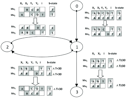
Figure 1. Example: Code and Barrier Diagram

In Figure 1 we give a pictorial representation of the state machine associated with the barrier used in the code using the following specialized notation:

This notation is used to express the pre- and postconditions for a given barrier transition. Each row is a pictorial representation (values, barrier states, and shares) of a formula in separation logic as indicated above. The preconditions are on top (one per row) and the postconditions below. Each row is associated with a move; move 1 is a pair of the first precondition row and the first postcondition row, etc. A barrier that is waiting for $n$ threads will have $n$ moves; $n$ can be fewer than the total number of threads. We do not require that a given thread always takes the same move each time it reaches a given barrier transition.

Note that only the permissions on the memory cells change during a transition; the contents (values) do not. The exception to this is the special column on the right side, which denotes the assertion associated with the barrier itself. As the barrier transitions, this value changes from the previous state to the next; we require that the sum of the preconditions includes the full share of the barrier assertion to guarantee that no thread has an out-of-date view of the barrier’s state. Observe that all of the preconditions join together, and, except for the state of the barrier itself, are exactly equal to the join of the postconditions.

The initial state of the machine is given as an assertion in line 0. The machine starts with full ownership of the array cells $x_{1}$, $x_{2}$, $y_{1}$, and $y_{2}$, as well as an additional cell $i$, used as a condition variable. The barrier b is fully-owned and is in state 0. The initial state is then partitioned into two parts on line 0’, with the left thread (A) and right thread (B) getting the shares ⬗ and ⬗ , respectively.

Not shown (between lines 0’ and 1) is thread-specific initialization code; perhaps both threads read both arrays and perform consistency checks. The real action starts with the barrier call on line 1, which ensures that this initialization code has completed. Thread A takes move 1 and thread B takes move 2. Afterwards, thread A has full ownership over $y_{1}$ and thread B has full ownership over $y_{2}$; the ownership of $x_{1}$, $x_{2}$, and $i$ remains split between A and B. While the ownership of the barrier is unchanged, it is now in state 1.

We then enter the main loop on line 3. On lines 4–5, both threads read from the shared cells $x_{1}$ and $x_{2}$, and on line 6 both threads update their fully-owned cell. The barrier call on line 7 ensures that these updates have been completed before the threads continue. Since the value T at memory location $i$ is less than 30, only the 1–2 transition is possible; the 1–3 transition requires T$\geq 30$. Thread A takes move 1 and thread B takes move 2; afterwards, both threads have partial shares of $y_{1}$ and $y_{2}$, thread A has the full share of $x_{1}$ and the condition cell $i$, and thread B has the full share of $x_{2}$; the barrier is in state 2.

Lines 8–10 are mirrors of lines 4–6. On lines 11–12, thread A updates the condition cell $i$. The barrier on line 13 ensures that the updates on lines 10 and 12 have completed before the threads continue; thread A takes move 2 while thread B takes move 1. Afterwards, the threads have the same permissions they had on entering the loop: A has full ownership of $y_{1}$, B has full ownership of $y_{2}$, and they share ownership of $x_{1}$, $x_{2}$, and $i$; the barrier is again in state 1.

On line 14, thread B reads from the condition variable $i$, and then the program loops back to line 3. After 30 iterations, the loop exits and control moves to the barrier on line 16. Observe that since the (shared) value T at memory location $i$ is greater than or equal to 30, only the 1–3 transition is possible; the 1–2 transition requires T$<30$. Thread A takes move 1 while thread B takes move 2; afterwards, both threads are sharing ownership of $x_{1}$, $x_{2}$, $y_{1}$, and $y_{2}$ (since the transition from 1 to 3 does not mention $y_{1}$ and $y_{2}$ they are unchanged). Thread A has full permission over the condition variable $i$; the barrier is in state 3. Finally, on line 17, thread A updates $i$; the barrier on line 16 ensures that thread B’s read of $i$ on line 14 has already occurred.

4. Barrier Definitions and Consistency Requirements

We present the type of a barrier definition in Figure 2 in the form of a data structure. The definitions include numerous consistency requirements; in Coq these are maintained with dependent types. From the top down, a barrier definition ($\mathsf{BarDef}$) consists of a barrier identifier (i.e., barrier number), the number of threads the barrier is synchronizing, and a list of barrier state definitions. For programs that have more than one barrier, the individual barrier definitions will be collected into a list and barrier number $j$ will be in list slot $j$.

$$\begin{array}[]{lclrl}\mathsf{BarDef}&\quad\equiv&\{~{}\mathsf{bd\_bn}:\mathit{Nat}&\mathrm{barrier~{}id}\\ \mathrm{(barrier~{}definition)}&&~{}~{}\mathsf{bd\_limit}:\mathit{Nat}&\qquad\mathrm{\#~{}of~{}threads}&\\ &&~{}~{}\mathsf{bd\_states}:\mathit{list}~{}\mathsf{BarStateDef}\}&\mathrm{state~{}list}\\ \mathsf{BarStateDef}&\equiv&\{\mathsf{bsd\_bn}:\mathit{Nat}&\mathrm{barrier~{}id}\\ \mathrm{(barrier~{}state)}&&~{}~{}\mathsf{bsd\_cs}:\mathit{Nat}&\mathrm{state~{}id}\\ &&~{}~{}\mathsf{bsd\_directions}:\mathit{list}~{}\mathsf{BarMoveList}&\mathrm{transition~{}list}\\ &&~{}~{}\mathsf{bsd\_limit}:\mathit{Nat}\}&\mathrm{\#~{}of~{}threads}\\ \mathsf{BarMoveList}&\equiv&\{\mathsf{bml\_ns}:\mathit{Nat}&\mathrm{next~{}state}\\ \mathrm{(transition)}&&~{}~{}\mathsf{bml\_bn}:\mathit{Nat}&\mathrm{barrier~{}id}\\ &&~{}~{}\mathsf{bml\_cs}:\mathit{Nat}&\mathrm{current~{}state}\\ &&~{}~{}\mathsf{bml\_limit}:\mathit{Nat}&\mathrm{\#~{}of~{}threads}\\ &&~{}~{}\mathsf{bml\_moves}:\mathit{list}~{}(\mathsf{assert}\times\mathsf{assert})\}&\mathrm{pre/post~{}pairs}\\ \end{array}$$

Figure 2. Barrier Definitions

A barrier state definition ($\mathsf{BarStateDef}$) consists of a barrier number, the number of threads synchronized, a state id, and a transition list; such that:

1. the barrier number matches the barrier number in the containing $\mathsf{BarDef}$

2. the limit matches the limit of the containing $\mathsf{BarDef}$

3. the state identifier $j$ indicates that this $\mathsf{BarStateDef}$ is the $j$ element of the containing $\mathsf{BarDef}$’s list of state definitions

4. the directions are mutually exclusive

The first three are unexciting; we will discuss mutual exclusion shortly.

A transition ($\mathsf{BarMoveList}$) contains a barrier number ($\mathsf{bn}$), number of threads synchronized, current state identifier ($\mathsf{cs}$), next state identifier ($\mathsf{ns}$), and list of precondition/postcondition pairs (the move list). We require that:

1. $\mathsf{bn}$ matches the barrier number in the containing $\mathsf{BarStateDef}$

2. the limit matches the limit in the containing $\mathsf{BarStateDef}$

3. $\mathsf{cs}$ matches the state identifier in the containing $\mathsf{BarStateDef}$

4. the length of list of moves ($\mathsf{bml\_moves}$) is equal to the limit ($\mathsf{bml\_limit}$)

5. all of the pre/postconditions in the movelist ignore the store, focusing only on the memory and barrier map. Since stores are private to each thread (on a processor these would be registers), it does not make sense for them to be mentioned in the “public” pre/post conditions.

6. all of the preconditions in the movelist are precise. Precision is a technical property involving the identifiability of states satisfying an assertion. An assertion $P$ is precise when

   $$\sigma_{1}=\sigma 1^{\prime}\sigma_{1}\oplus\sigma_{2}=\sigma_{3}\qquad\sigma_{1}\models P\qquad\sigma_{1}^{\prime}\oplus\sigma_{2}^{\prime}=\sigma_{3}\qquad\sigma_{1}^{\prime}\models P$$

   That is, $P$ can hold on at most one substate of an arbitrary state $\sigma_{3}$.

7. each precondition $P$ includes some positive share of the $\mathsf{barrier}$ assertion with $\mathsf{bn}$ and $\mathsf{cs}$, i.e., $\exists\pi.~{}P\Rightarrow\top~{}{{\tt*}}~{}\mathsf{barrier}(\mathit{\mathsf{bn}},\pi,\mathit{\mathsf{cs}})$.

8. the sum of the preconditions must equal the sum of the postconditions, except for the state of the barrier; moreover, the sum of the preconditions must include the full share of the barrier (equation (2), repeated here):

   $$\begin{array}[]{lcl}\raisebox{-7.0pt}{$\stackrel{{\scriptstyle\mbox{\huge{{$\tt*$}}}}}{{{}_{i}}}$}~{}{\vspace{-10pt}\mathit{Pre}_{i}}&\qquad=&F~{}{{\tt*}}~{}\mathsf{barrier}(\mathit{\mathsf{bn}},\raisebox{0.5pt}{\rotatebox[origin={c}]{90.0}{\leavevmode\resizebox{5.97508pt}{5.97508pt}{{\char 96\relax}}}},\mathit{\mathsf{cs}})\\[5.0pt] \raisebox{-7.0pt}{$\stackrel{{\scriptstyle\mbox{\huge{{$\tt*$}}}}}{{{}_{i}}}$}~{}{\vspace{-10pt}\mathit{Post}_{i}}&=&F~{}{{\tt*}}~{}\mathsf{barrier}(\mathit{\mathsf{bn}},\raisebox{0.5pt}{\rotatebox[origin={c}]{90.0}{\leavevmode\resizebox{5.97508pt}{5.97508pt}{{\char 96\relax}}}},\mathit{\mathsf{ns}})\end{array}$$

Items 1–4 are simple bookkeeping; items 5–7 are similar to technical requirements required in other variants of concurrent separation logic [29, 21, 20]. As previously mentioned, the fundamental insight of this approach is property (8).

The function $\mathsf{lookup\_move}$ simplifies the lookup of a move in a $\mathsf{BarDef}$:

$$\mathsf{lookup\_move}(\mathit{bd},\mathit{cs},\mathit{dir},\mathit{mv})=bd.\mathsf{bd\_states}[\mathit{cs}].\mathsf{bsd\_directions}[\mathit{dir}].\mathsf{bml\_moves}[\mathit{mv}]$$

Using this notation, we can express the important requirement that all directions in the barrier state $\mathit{cs}$ of the barrier definition $\mathsf{bd}$ are mutually exclusive:

$$\begin{array}[]{l}\forall\mathit{dir}_{1},\mathit{dir}_{2},\mathit{mv}_{1},\mathit{mv}_{2},\mathit{pre}_{1},\mathit{pre}_{2}.~{}\mathit{dir}_{1}\neq\mathit{dir}_{2}~{}\Rightarrow\\ ~{}~{}\mathsf{lookup\_move}(\mathit{bd},\mathit{cs},\mathit{dir}_{1},\mathit{mv}_{1})=(\mathit{pre}_{1},\underline{~{}~{}})~{}\Rightarrow\\ ~{}~{}~{}~{}\mathsf{lookup\_move}(\mathit{bd},\mathit{cs},\mathit{dir}_{2},\mathit{mv}_{2})=(\mathit{pre}_{2},\underline{~{}~{}})~{}\Rightarrow\\[3.0pt] ~{}~{}~{}~{}~{}~{}~{}~{}(\top~{}{{\tt*}}~{}\mathit{pre}_{1})~{}\wedge~{}(\top~{}{{\tt*}}~{}\mathit{pre}_{2})~{}~{}\equiv~{}~{}\bot\end{array}$$

In other words, it is impossible for any of the preconditions of more than one transition (of a given state) to be true at a time. The simplest way to understand this is to consider the 1–2 and 1–3 transitions in the example program. The 1–2 transition requires that the value in memory cell $i$ be strictly less than 30; in contrast, the 1–3 transition requires that the same cell contains a value greater than or equal to 30. Plainly these are incompatible; but in fact the above property is stronger: both of the moves on the 1–2 transition, and both of the moves on the 1–3 transition include the incompatibility. Thus, if thread A takes transition 1–2, it knows for certain that thread B cannot take transition 1–3. This way we ensure that both threads always agree on the barrier’s current state.

5. Hoare Logic

Our Hoare judgment has the form $\Gamma\vdash\{P\}~{}c~{}\{Q\}$, where $\Gamma$ is a list of barrier definitions as given in §4, $P$ and $Q$ are assertions in separation logic, and $c$ is a command. Our Hoare rules come in three groups: standard Hoare logic (Skip, If, Sequence, While, Assignment, Consequence); standard separation logic (Frame, Store, Load, New, Free); and the barrier rule. We give all three groups two and three in Figure 3. We note four points for group two.

$$\begin{array}[]{c}\Gamma\vdash\{P\}~{}\texttt{skip}~{}\{P\}\qquad\Gamma\vdash\{P\}~{}{{\tt if}}~{}e~{}{{\tt then}}~{}c_{t}~{}{{\tt else}}~{}c_{f}~{}\{Q\}\Gamma\vdash\{P~{}{{\tt*}}~{}[e]\}~{}c_{t}~{}\{Q\}\quad\Gamma\vdash\{P~{}{{\tt*}}~{}\neg[e]\}~{}c_{f}~{}\{Q\}\\ \\ \\ \Gamma\vdash\{P\}~{}c_{1}~{};~{}c_{2}~{}\{R\}\Gamma\vdash\{P\}~{}c_{1}~{}\{Q\}\quad\Gamma\vdash\{Q\}~{}c_{2}~{}\{R\}\quad\Gamma\vdash\{I\}~{}{{\tt while}}~{}e~{}\{c\}~{}\{I~{}{{\tt*}}~{}\neg[e]\}\Gamma\vdash\{I~{}{{\tt*}}~{}[e]\}~{}c~{}\{I\}\\ \\ \Gamma\vdash\{e\Downarrow v\}~{}x~{}{{\tt:=}}~{}e~{}\{x=v\}\quad\Gamma\vdash\{P^{\prime}\}~{}c~{}\{Q^{\prime}\}P^{\prime}\vdash P~{}~{}\Gamma\vdash\{P\}~{}c~{}\{Q\}~{}~{}Q\vdash Q^{\prime}\\ \\ \Gamma\vdash\{F~{}{{\tt*}}~{}P\}~{}c~{}\{F~{}{{\tt*}}~{}Q\}\Gamma\vdash\{P\}~{}c~{}\{Q\}~{}~{}\mathsf{closed}(F,c)~{}~{}~{}~{}\Gamma\vdash\{e_{1}{\xmapsto{\raisebox{0.5pt}{\rotatebox[origin={c}]{90.0}{\leavevmode\resizebox{5.97508pt}{5.97508pt}{{\char 96\relax}}}}}}\_\}~{}{{\tt[}}e_{1}{{\tt]}}~{}{{\tt:=}}~{}e_{2}~{}\{e_{1}{\xmapsto{\raisebox{0.5pt}{\rotatebox[origin={c}]{90.0}{\leavevmode\resizebox{5.97508pt}{5.97508pt}{{\char 96\relax}}}}}}e_{2}\}~{}\\ \\ \Gamma\vdash\{e_{1}{\xmapsto{\pi}}e_{2}~{}{{\tt*}}~{}e_{1}\Downarrow v_{1}~{}{{\tt*}}~{}e_{2}\Downarrow v_{2}\}~{}x~{}{{\tt:=}}~{}{{\tt[}}e_{1}{{\tt]}}~{}\{\texttt{C}(v_{1}){\xmapsto{\pi}}\texttt{C}(v_{2})~{}{{\tt*}}~{}x=v_{2}\}\\ \\ \Gamma\vdash\{e\Downarrow v\}~{}x{{\tt:=}}~{}{{\tt new}}~{}e~{}\{\texttt{V}(x){\xmapsto{\raisebox{0.5pt}{\rotatebox[origin={c}]{90.0}{\leavevmode\resizebox{5.97508pt}{5.97508pt}{{\char 96\relax}}}}}}\texttt{C}(v)\}~{}~{}\Gamma\vdash\{e_{1}{\xmapsto{\raisebox{0.5pt}{\rotatebox[origin={c}]{90.0}{\leavevmode\resizebox{5.97508pt}{5.97508pt}{{\char 96\relax}}}}}}e_{2}\}~{}{{\tt free}}~{}e_{1}~{}\{\mathsf{emp}\}\\ \\ \framebox{ $\Gamma\vdash\{\mathit{P}\}~{}{\bf{{\tt\bf barrier}}}~{}bn~{}\{\mathit{Q}\}\Gamma[\mathit{bn}]=\mathit{bd}\qquad\mathsf{lookup\_move}(\mathit{bd},\mathit{cs},\mathit{dir},\mathit{mv})=(P,Q)$ }\end{array}$$

Figure 3. Hoare rules

First, as explained in §2.4, the assertions $e\Downarrow v$, $[e]$ and $x=v$ are bundled with an assertion that the heap and barrier map are empty(i.e., $e\Downarrow v~{}~{}\Rightarrow~{}~{}\mathsf{emp}$); thus, we use the separating conjunction when employing them. Second, the rules are in “side-condition-free form”. Thus, instead of presenting the load rule as $\Gamma\vdash\{e_{1}{\xmapsto{\pi}}e_{2}\}~{}x~{}{{\tt:=}}~{}{{\tt[}}e_{1}{{\tt]}}~{}\{x=e_{2}~{}{{\tt*}}~{}e_{1}{\xmapsto{\pi}}e_{2}\}$, which is aesthetically attractive but untrue in the pesky case when $e_{2}$ depends on $x$ (e.g., $x~{}{{\tt:=}}~{}{{\tt[}}x{{\tt]}}$), we use a form that is less visually pleasing but does not require side conditions. It is straightforward to restore rules with side conditions via the Consequence rule. Third, our Store and Free rules require the full share of location $e_{1}$; in contrast, our Load rule only requires some positive share; this is consistent with our use of fractional permissions as explained in §2.3. Fourth, memory allocation and deallocation are more complicated in concurrent settings than in sequential settings, and so the New and Free rules cause nontrivial complications in the semantic model.

The Hoare rule for barriers is so simple that at first glance it may be hard to understand. The variables for the current state $\mathit{cs}$, direction $\mathit{dir}$, and move $\mathit{mv}$ appear to be free in the $\mathsf{lookup\_move}$! However, things are not quite as unconstrained as they initially appear. Recall from §4 that one of the consistency requirements for the precondition $P$ is that $P$ implies an assertion about the barrier itself: $P\Rightarrow Q~{}{{\tt*}}~{}\mathsf{barrier}(\mathit{\mathit{bn}},\pi,\mathit{\mathit{cs}})$; thus at a given program point we can only use directions and moves from the current state. Similarly, recall from §4 that since the directions are mutually exclusive, $\mathit{dir}$ is uniquely determined.

This leaves the question of the uniqueness of $\mathit{mv}$. If a thread only satisfies a single precondition, then the move $\mathit{mv}$ is uniquely determined. Unfortunately, it is simple to construct programs in which a thread enters a barrier while satisfying the preconditions of multiple moves. What saves us is that we are developing a logic of partial correctness. Since preconditions to moves must be precise and nonempty (i.e., token), only one thread is able to satisfy a given precondition at a time. The pigeonhole principle guarantees that if a thread holds multiple preconditions then some other thread will not be able to enter the barrier; in this case, the barrier call will never return and we can guarantee any postcondition.

We now apply the Barrier rule to the barrier calls in line 13 from our example program; the $\mathsf{lookup\_move}$s are direct from the barrier state diagram:

$$\begin{array}[]{l}\mathsf{Thread~{}A}~{}\begin{cases}\Gamma\vdash\{P\}~{}{\bf{{\tt\bf barrier}}}~{}b~{}\{Q\}\begin{array}[]{c}\mathsf{lookup\_move}(b,2,1,2)=(P,Q)\\ P=y_{1}{\xmapsto{\raisebox{-1.0pt}{\rotatebox[origin={c}]{135.0}{\leavevmode\resizebox{8.53581pt}{8.53581pt}{{\char 63\relax}}}}}}v_{y1}~{}{{\tt*}}~{}y_{2}{\xmapsto{\raisebox{-1.0pt}{\rotatebox[origin={c}]{135.0}{\leavevmode\resizebox{8.53581pt}{8.53581pt}{{\char 63\relax}}}}}}v_{y2}~{}{{\tt*}}~{}x_{1}{\xmapsto{\raisebox{0.5pt}{\rotatebox[origin={c}]{90.0}{\leavevmode\resizebox{5.97508pt}{5.97508pt}{{\char 96\relax}}}}}}v_{x1}~{}{{\tt*}}~{}i{\xmapsto{\raisebox{0.5pt}{\rotatebox[origin={c}]{90.0}{\leavevmode\resizebox{5.97508pt}{5.97508pt}{{\char 96\relax}}}}}}v_{i}{{\tt*}}\mathsf{barrier}(\mathit{bn},\raisebox{-1.0pt}{\rotatebox[origin={c}]{135.0}{\leavevmode\resizebox{8.53581pt}{8.53581pt}{{\char 63\relax}}}},\mathit{2})\\ Q=y_{1}{\xmapsto{\raisebox{0.5pt}{\rotatebox[origin={c}]{90.0}{\leavevmode\resizebox{5.97508pt}{5.97508pt}{{\char 96\relax}}}}}}v_{y1}~{}{{\tt*}}~{}x_{1}{\xmapsto{\raisebox{-1.0pt}{\rotatebox[origin={c}]{135.0}{\leavevmode\resizebox{8.53581pt}{8.53581pt}{{\char 63\relax}}}}}}v_{x1}~{}{{\tt*}}~{}x_{2}{\xmapsto{\raisebox{-1.0pt}{\rotatebox[origin={c}]{135.0}{\leavevmode\resizebox{8.53581pt}{8.53581pt}{{\char 63\relax}}}}}}v_{x2}~{}{{\tt*}}~{}i{\xmapsto{\raisebox{-1.0pt}{\rotatebox[origin={c}]{135.0}{\leavevmode\resizebox{8.53581pt}{8.53581pt}{{\char 63\relax}}}}}}v_{i}{{\tt*}}\mathsf{barrier}(\mathit{bn},\raisebox{-1.0pt}{\rotatebox[origin={c}]{135.0}{\leavevmode\resizebox{8.53581pt}{8.53581pt}{{\char 63\relax}}}},\mathit{1})\\ \end{array}\end{cases}\\ \mathsf{Thread~{}B}~{}\begin{cases}\Gamma\vdash\{P\}~{}{\bf{{\tt\bf barrier}}}~{}b~{}\{Q\}\begin{array}[]{c}\mathsf{lookup\_move}(b,2,1,1)=(P,Q)\\ P=y_{1}{\xmapsto{\raisebox{-1.0pt}{\rotatebox[origin={c}]{315.0}{\leavevmode\resizebox{8.53581pt}{8.53581pt}{{\char 63\relax}}}}}}v_{y1}~{}{{\tt*}}~{}y_{2}{\xmapsto{\raisebox{-1.0pt}{\rotatebox[origin={c}]{315.0}{\leavevmode\resizebox{8.53581pt}{8.53581pt}{{\char 63\relax}}}}}}v_{y2}~{}{{\tt*}}~{}x_{2}{\xmapsto{\raisebox{0.5pt}{\rotatebox[origin={c}]{90.0}{\leavevmode\resizebox{5.97508pt}{5.97508pt}{{\char 96\relax}}}}}}v_{x2}{{\tt*}}\mathsf{barrier}(\mathit{bn},\raisebox{-1.0pt}{\rotatebox[origin={c}]{315.0}{\leavevmode\resizebox{8.53581pt}{8.53581pt}{{\char 63\relax}}}},\mathit{2})\}\vspace{3pt}\\ Q=y_{2}{\xmapsto{\raisebox{0.5pt}{\rotatebox[origin={c}]{90.0}{\leavevmode\resizebox{5.97508pt}{5.97508pt}{{\char 96\relax}}}}}}v_{y2}~{}{{\tt*}}~{}x_{1}{\xmapsto{\raisebox{-1.0pt}{\rotatebox[origin={c}]{315.0}{\leavevmode\resizebox{8.53581pt}{8.53581pt}{{\char 63\relax}}}}}}v_{x1}~{}{{\tt*}}~{}x_{2}{\xmapsto{\raisebox{-1.0pt}{\rotatebox[origin={c}]{315.0}{\leavevmode\resizebox{8.53581pt}{8.53581pt}{{\char 63\relax}}}}}}v_{x2}~{}{{\tt*}}~{}i{\xmapsto{\raisebox{-1.0pt}{\rotatebox[origin={c}]{315.0}{\leavevmode\resizebox{8.53581pt}{8.53581pt}{{\char 63\relax}}}}}}v_{i}{{\tt*}}\mathsf{barrier}(\mathit{bn},\raisebox{-1.0pt}{\rotatebox[origin={c}]{315.0}{\leavevmode\resizebox{8.53581pt}{8.53581pt}{{\char 63\relax}}}},\mathit{1})\}\\ \end{array}\end{cases}\\ \end{array}$$

Note that in this line of the example program, the frame is $\mathsf{emp}$ in both threads.

Not shown in Figure 3 is a parallel composition rule. As in [21], each thread is verified independently using the Hoare rules given; a top-level safety theorem proves that the entire concurrent machine behaves as expected.

6. Semantic Models

Our operational semantics is divided into three parts: purely sequential, which executes all of the instructions except for barrier in a thread-local manner; concurrent, which manages thread scheduling and handles the barrier instruction; and oracular, which provides a pseudosequential view of the concurrent machine to enable simple proofs of the sequential Hoare rules. Our setup follows Hobor et al. very closely and we refer readers there for more detail [22, 21].

Purely sequential semantics.

The purely sequential semantics executes the instructions skip, $x$ $\tt:=$ $e$, $x$ $\tt:=$ $\tt[$$e$$\tt]$, $\tt[$$e_{1}$$\tt]$ $\tt:=$ $e_{2}$, $x$$\tt:=$ $\tt new$ $e$, $\tt free$ $e$, $c_{1}$;  $c_{2}$, if $e$ then $c_{1}$ else $c_{2}$, and $\tt while$ $e$ {$c$}. The form of the sequential step judgment is $(\sigma,c)\mapsto(\sigma^{\prime},c^{\prime})$. Here $\sigma$ is a state (triple of store, heap, barrier map), just as in §2.4 and $c$ is a command of our language. The semantics of the sequential instructions is standard; the only “tricky” part is that the machine gets stuck if one tries to write to a location for which one does not have full permission or read from a location for which one has no permission; e.g., here is the store rule:

$$\big{(}(s,h,b),~{}{{\tt[}}e_{1}{{\tt]}}~{}{{\tt:=}}~{}e_{2}{{\tt;}}~{}c\big{)}~{}\mapsto~{}\big{(}(s,h^{\prime},b),c\big{)}\begin{array}[]{c}s\vdash e_{1}\Downarrow\texttt{C}(\texttt{ADDR}(n))\qquad s\vdash e_{2}\Downarrow v\\ n<\mathsf{break}(h)\qquad h(n)=(\raisebox{0.5pt}{\rotatebox[origin={c}]{90.0}{\leavevmode\resizebox{5.97508pt}{5.97508pt}{{\char 96\relax}}}},v^{\prime})\qquad h^{\prime}=[n\mapsto(\raisebox{0.5pt}{\rotatebox[origin={c}]{90.0}{\leavevmode\resizebox{5.97508pt}{5.97508pt}{{\char 96\relax}}}},v)]h\end{array}$$

The test that $n<\mathsf{break}(h)$ ensures that the address for the store is “in bounds”—that is, less than the current value of the break between allocated and unallocated memory; since we are updating the memory we require that the permission associated with the location $n$ be full ( ◼ ). We say that this step relation is unerased since these bounds and permission checks are virtual rather than on-chip.

We define the other cases of the step relation in a similar way. Observe that if we were in a sequential setting the proof of the Hoare store rule would be straightforward; this is likewise the case for the other cases of the sequential step relation and their associated Hoare rules. If the sequential step relation reaches a barrier call $\tt\bf barrier$ $\mathsf{bn}$ then it simply gets stuck.

Concurrent semantics.

We define the notion of a concurrent state in Figure 4. A concurrent state contains a scheduler $\Omega$ (modeled as a list of natural numbers), a distinguished heap called the allocation pool, a list of threads, and a barrier pool. The allocation pool “owns” all of the unallocated memory cells and the “break” that indicates the division between allocated and unallocated cells. Before we run a thread we transfer the allocation pool into the local heap owned by the thread so that new can transfer a cell from this pool into the local heap of a thread when required. When we suspend the thread we remove (what is left of) the allocation pool from its heap so that we can transfer it to the next thread.

A thread contains a (sequential) state (store, heap, and barrier map) and a concurrent control, which is either $\mathsf{Running}(c)$, meaning the thread is available to run command $c$, or $\mathsf{Waiting}(\mathit{bn},\mathit{dir},\mathit{mv},c)$, meaning that the thread is currently waiting on barrier $\mathit{bn}$ to make move $\mathit{mv}$ in direction $\mathit{dir}$; after the barrier call completes the thread will resume running with command $c$.

$$\begin{array}[]{lclr}\mathsf{Cstate}&\quad\equiv&\{~{}\mathsf{cs\_sched}:\mathsf{list~{}\mathbb{N}}&\mathrm{schedule}\\ &&~{}~{}\mathsf{cs\_allocpool}:\mathsf{heap}&\mathrm{alloc~{}pool}\\ &&~{}~{}\mathsf{cs\_thds}:\mathsf{list}~{}\mathsf{Thread}&\mathrm{thread~{}pool}\\ &&~{}~{}\mathsf{cs\_barpool}:\mathsf{Barpool}\}&\mathrm{barrier~{}pool}\\[3.0pt] \mathsf{Thread}&\quad\equiv&\{~{}\mathsf{th\_stk}:\mathsf{store}&\\ &&~{}~{}\mathsf{th\_hp}:\mathsf{heap}&\\ &&~{}~{}\mathsf{th\_bs}:\mathsf{BarrierMap}&\mathrm{local~{}view~{}of~{}barrier~{}states}\\ &&~{}~{}\mathsf{th\_ctl}:\mathsf{conc\_ctl}\}&\mathrm{running~{}or~{}waiting}\\[3.0pt] \mathsf{conc\_ctl}&\quad\equiv&|\mathsf{~{}Running}(c)&\mathrm{executing~{}code~{}c}\\ &&|\mathsf{~{}Waiting}(bn,dir,mv,c)&\mathrm{waiting~{}on~{}bn}\\[3.0pt] \mathsf{Barpool}&\quad\equiv&\{~{}\mathsf{bp\_bars}:\mathsf{list}~{}\mathsf{DyBarStatus}&\quad\mathrm{dynamic~{}barrier~{}status}\\ &&~{}~{}\mathsf{bp\_st}:\mathsf{store\times heap\times BarrierMap}\}&\mathrm{current~{}state}\\[3.0pt] \mathsf{DyBarStatus}&\quad\equiv&\{~{}\mathsf{dbs\_bn}:\mathit{\mathbb{N}}&\mathrm{barrier~{}id}\\ &&~{}~{}\mathsf{dbs\_wp}:\mathsf{Waitpool}&\mathrm{waiting~{}thread~{}pool}\\ &&~{}~{}\mathsf{dbs\_bd}:\mathsf{BarDef}\}&\\[3.0pt] \mathsf{Waitpool}&\quad\equiv&\{~{}\mathsf{wp\_dir}:\mathit{option~{}\mathbb{N}}&\mathrm{direction~{}id}\\ &&~{}~{}\mathsf{wp\_slots}:\mathit{option~{}}(\mathsf{list~{}}\mathsf{slot})&\mathrm{taken~{}slots}\\ &&~{}~{}\mathsf{wp\_limit}:\mathit{\mathbb{N}}&\\ &&~{}~{}\mathsf{wp\_st}:\mathsf{store\times heap\times BarrierMap}\}&\mathrm{current~{}state}\\[3.0pt] \mathsf{slot}&\quad\equiv&\mathsf{(thread\_id\times heap\times BarrierMap)}&\qquad\qquad\mathrm{waiting~{}slot}\\ \end{array}$$

Figure 4. Concurrent state

The barrier pool ($\mathsf{Barpool}$) contains a list of dynamic barrier statuses (DBSes) as well as a state which is the join of all of the states inside the DBSes. Each DBS consists of a barrier number (which must be its index into the array of its containing $\mathsf{Barpool}$), a barrier definition (from §4), and a waitpool (WP). A waitpool consists of a direction option (None before the first barrier call in a given state; thereafter the unique direction for the next state), a limit (the number of threads synchronized by the barrier, and comes from the barrier definition in the enclosing DBS), a slot list, and a state (which is the join of all of the states in the slot list). A slot is a heap and barrier map (the store is unneeded since barrier pre/postconditions ignore it) as well as a thread id (whence the heap and barrier map came as a precondition, and to which the postcondition will return).

The concurrent step relation has the form $(\Omega,\mathit{ap},\mathit{thds},\mathit{bp})\leadsto(\Omega^{\prime},\mathit{ap}^{\prime},\mathit{thds}^{\prime},\mathit{bp}^{\prime})$, where $\Omega$, $\mathit{ap}$, $\mathit{thds}$, and $\mathit{bp}$ are the scheduler, allocation pool, thread list, and barrier pool respectively. The concurrent step relation has only four cases; the following case CStep-Seq is used to run all of the sequential commands:

$$(i::\Omega,\mathit{thds},\mathit{ap},\mathit{bp})\leadsto(i::\Omega,\mathit{thds}^{\prime},\mathit{ap}^{\prime},\mathit{bp})\begin{array}[]{c}\mathit{thds}[i]=(s,h,b,\mathsf{Running}(c))\qquad h\oplus\mathit{ap}=h^{\prime}\qquad\big{(}(s,h^{\prime},b),c\big{)}\mapsto\big{(}(s^{\prime},h^{\prime\prime},b),c^{\prime}\big{)}\\ h^{\prime\prime\prime}\oplus\mathit{ap}^{\prime}=h^{\prime\prime}\qquad\mathsf{isAllocPool}(\mathit{ap}^{\prime})\qquad\mathit{thds}^{\prime}=[i\mapsto(s^{\prime},h^{\prime\prime\prime},b,\mathsf{Running}(c^{\prime}))]\mathit{thds}\end{array}$$

That is, we look up the thread whose thread id is at the head of the scheduler, join in the allocation pool, and run the sequential step relation. If the command $c$ is a barrier call then the sequential relation will not be able to run and so the CStep-Seq relation will not hold; otherwise the sequential step relation will be able to handle any command. After we have taken a sequential step, we subtract out the (possibly diminished) allocation pool, and reinsert the modified sequential state into the thread list. Since we quantify over all schedulers and our language does not have input/output, it is sufficient to utilize a non-preemptive scheduler; for further justification on the use of such schedulers see [21].

The second case of the concurrent step relation handles the case when a thread has reached the last instruction, which must be a skip:

$$(i::\Omega,\mathit{thds},\mathit{ap},\mathit{bp})\leadsto(\Omega,\mathit{thds},\mathit{ap},\mathit{bp})\mathit{thds}[i]=\mathsf{Running}(\texttt{skip})$$

When we reach the end of a thread we simply context switch to the next thread.

The interesting cases occur when the instruction for the running thread is a barrier call; here the CStep-Seq rule does not apply. The concurrent semantics handles the barrier call directly via the last two cases of the step relation; before presenting these cases we will first give a technical definition called $\mathsf{fill\_barrier\_slot}$:

$$\mathsf{fill\_barrier\_slot}~{}~{}(thds,~{}bp,~{}bn,~{}i)=(thds^{\prime},~{}bp^{\prime})\begin{array}[]{c}thds[i]=\mathsf{Thread}(stk,~{}hp,~{}bs,~{}(\mathsf{Running}~{}({\bf{{\tt\bf barrier}}}~{}bn;~{}c)))\\[2.0pt] \mathsf{lookup\_move}(bp.bp\_bars[bn],~{}dir,~{}mv)=(pre,post)\\ hp^{\prime}\oplus hp^{\prime\prime}=hp\qquad\quad bs^{\prime}\oplus bs^{\prime\prime}=bs\qquad\quad pre(stk,hp^{\prime},bs^{\prime})\\[2.0pt] \mathsf{bp\_inc\_waitpool}~{}(bp,~{}bn,~{}dir,~{}mv,~{}(i,~{}(hp^{\prime},~{}bs^{\prime})))=bp^{\prime}\\[2.0pt] thds^{\prime}=[i\rightarrow(\mathsf{Thread}(~{}stk,~{}hp^{\prime\prime},~{}bs^{\prime\prime},~{}(\mathsf{Waiting}~{}(bn,~{}dir,~{}mv,~{}c))))]~{}thds\\ \end{array}$$

The predicate $\mathsf{fill\_barrier\_slot}$ gives the details of removing the (sub)state satisfying the precondition of the barrier from the thread’s state, inserting it into the barrier pool, and suspending the calling thread. The predicate $\mathsf{bp\_inc\_waitpool}$ does the insertion into the barrier pool; the details of manipulating the data structure are straightforward but lengthy to formalize.

We are now ready to give the first case for the barrier, used when a thread executes a barrier but is not the last thread to do so:

$$((i::\Omega),ap,thds,bp)\leadsto(\Omega,ap,thds^{\prime},bp^{\prime})\begin{array}[]{c}\mathsf{fill\_barrier\_slot}~{}~{}(thds,~{}bp,~{}bn,~{}i)=(thds^{\prime},~{}bp^{\prime})\\ \neg~{}\mathsf{bp\_ready}~{}~{}(bp^{\prime},~{}bn)\\ \end{array}$$

After using $\mathsf{fill\_barrier\_slot}$, CStep-Suspend checks to see if the barrier is full by counting the number of slots that have been filled in the appropriate wait pool by using the $\mathsf{bp\_ready}$ predicate, and then context switches.

If the barrier is ready then instead of using the CStep-Suspend case of the concurrent step relation, we must use the CStep-Release case:

$$((i::\Omega),ap,thds,bp)\leadsto(\Omega,ap,thds^{\prime\prime},bp^{\prime\prime})\begin{array}[]{c}\mathsf{fill\_barrier\_slot}~{}~{}(thds,~{}bp,~{}bn,~{}i)=(thds^{\prime},~{}bp^{\prime})\\ \mathsf{bp\_ready}~{}~{}(bp^{\prime},~{}bn)\\ \mathsf{bp\_transition}~{}~{}(bp^{\prime},~{}bn,~{}out)=bp^{\prime\prime}\\ \mathsf{transition\_threads}~{}~{}(out,~{}thds^{\prime})=thds^{\prime\prime}\\ \end{array}$$

The first requirement of CStep-Release is exactly the same as CStep-Suspend: we suspend the thread and transfer the appropriate resources to the barrier pool. However, now all of the threads have arrived at the barrier and so it is ready. We use the $\mathsf{bp\_transition}$ predicate to go through the barrier’s slots in the $\mathsf{waitpool}$, combine the associated heaps and barrier maps, redivide these resources according to the barrier postconditions, and remove the associated resources from the barrier pool into a list of slots called $\mathsf{out}$. Finally, the states in $\mathsf{out}$ are combined with the suspended threads, which are simultaneously resumed by the $\mathsf{transition\_threads}$ predicate. The formal definitions of the $\mathsf{bp\_transition}$ and $\mathsf{transition\_threads}$ predicates are extremely complex and very tedious and we refer interested readers to the mechanization.

Oracle semantics.

Following Hobor et al. [22, 21], we define a third oracular semantics: $(\sigma,o,c)\mapsto(\sigma^{\prime},o^{\prime},c^{\prime})$. Here the sequential state $\sigma$ and command $c$ are exactly the same as in the purely sequential step. The new parameter $o$ is an oracle, a kind of box containing “the rest” of the concurrent machine—that is, $o$ contains a scheduler, a list of other threads, and a barrier pool.

The oracle semantics behaves exactly the same way as the purely sequential semantics on all of the instructions except for the barrier call, with the oracle $o$ being passed through unchanged. That is to say:

$$\big{(}\sigma,o,c\big{)}~{}\mapsto~{}\big{(}\sigma^{\prime},o,c^{\prime}\big{)}\big{(}\sigma,c\big{)}~{}\mapsto~{}\big{(}\sigma^{\prime},c^{\prime}\big{)}$$

When the oracle semantics reaches a barrier instruction, it consults the oracle $o$ to determine the state of the machine after the barrier:

$$\big{(}(s,h,b),o,{\bf{{\tt\bf barrier}}}~{}\mathsf{bn}{{\tt;}}~{}c\big{)}~{}\mapsto~{}\big{(}(s,h^{\prime},b^{\prime}),o^{\prime},c\big{)}\mathsf{consult}(h,b,o)=(h^{\prime},b^{\prime},o^{\prime})$$

The formal definition of the $\mathsf{consult}$ relation is detailed in [22, 21] but the idea is simple. To consult the oracle, one unpacks the concurrent machine and runs (classically) all of the other threads until control returns to the original thread; consult then returns the current $h^{\prime}$ and $b^{\prime}$ (that resulted from the barrier call) and repackages the concurrent machine into the new oracle $o^{\prime}$. The final case of the oracle semantics occurs when the concurrent machine never returns control (because it got stuck or due to sheer perversion of the scheduler):

$$\big{(}(s,h,b),o,{\bf{{\tt\bf barrier}}}~{}\mathsf{bn}{{\tt;}}~{}c\big{)}~{}\mapsto~{}\big{(}(s,h,b),o,{\bf{{\tt\bf barrier}}}~{}\mathsf{bn}{{\tt;}}~{}c\big{)}\raisebox{1.0pt}{$\not$}\exists r.~{}\mathsf{consult}(h,b,o)=r\qquad\textrm{(\emph{i.e.}, $\mathsf{consult}$ diverges)}$$

When control will never return, it does not matter what this thread does as long as it does not get stuck; accordingly we enter an (infinite) loop.

Soundness proof outline.

Our soundness argument falls into several parts. We define our Hoare tuple in terms of our oracle semantics using a definition by Appel and Blazy [3]; this definition was designed for a sequential language and we believe that other standard sequential definitions for Hoare tuples would work as well. We then prove (in Coq) all of the Hoare rules for the sequential instructions; since the os-seq case of the oracle semantics provides a straight lift into the purely sequential semantics this is straightforward.

Next, we prove (in Coq) the soundness for the barrier rule. This turns out to be much more complicated than a proof of the soundness of (non-first-class) locks and took the bulk of the effort. There are two points of particular difficulty: first, the excruciatingly painful accounting associated with tracking resources during the barrier call as they move from a source thread (as a precondition), into the barrier pool, and redistribution to the target thread(s) as postcondition(s). The second difficulty is proving that a thread that enters a barrier while holding more than one precondition will never wake up; the analogy is a door with $n$ keys distributed among $n$ owners; if an owner has a second key in his pocket when he enters then one of the remaining owners will not be able to get in.

After proving the Hoare rules from Figure 3 sound with respect to the oracle semantics, the remaining task is to connect the oracle semantics to the concurrent semantics—that is, oracle soundness. Oracle soundness says that if each of the threads on a machine are safe with respect to the oracle semantics, then the entire concurrent machine combining the threads together is safe. The (very rough) analogy to this result in Brookes’ semantics is the parallel decomposition lemma. Here we use a progress/preservation style proof closely following that given in [21, pp.242–255]; the proof was straightforward and quite short to mechanize. A technical advance over previous work is that the progress/preservation proofs do not require that the concurrent semantics be deterministic. In fact, allowing the semantics to be nondeterministic simplified the proofs significantly.

A direct consequence of oracle soundness is that if each thread is verified with the Hoare rules, and is loaded onto a single concurrent machine, then if the machine does not get stuck and if it halts then all of the postconditions hold.

Erasure.

One can justly observe that our concurrent semantics is not especially realistic; e.g., we: explicitly track resource ownership permissions (i.e., our semantics is unerased); have an unrealistic memory allocator/deallocator and scheduler; ignore issues of byte-addressable memory; do not store code in the heap; and so forth. We believe that we could connect our semantics to a more realistic semantics that could handle each of these issues, but most of them are orthogonal to barriers. For brevity we will comment only on erasing the resource accounting since it forms the heart of our soundness result.

We have defined, in Coq, an erased sequential and concurrent semantics. An erased memory is simply a pair of a break address and a total function from addresses to values. The run-time state of an erased barrier is simply a pair of naturals: the first tracking the number of threads currently waiting on the barrier, and the second giving the final number of threads the barrier is waiting for. We define a series of $\mathsf{erase}$ functions that take an unerased type (memory/barrier status/thread/etc.) to an erased one by “forgetting” all permission information. The sequential erased semantics is quite similar to the unerased one, with the exception that we do not check if we have read/write permission before executing a load/store. The concurrent erased semantics is much simpler than the complicated accounting-enabled semantics explained above since all that is needed to handle the barrier is incrementing/resetting a counter, plus some modest management of the thread list to suspend/resume threads. Critically, our erased semantics is a computable function, enabling program evaluation. Finally, we have proved that our unerased semantics is a conservative approximation to our erased one: that is, if our unerased concurrent machine can take a step from some state $\Sigma$ to $\Sigma^{\prime}$, then our erased machine takes a step from $\mathsf{erase}(\Sigma)$ to $\mathsf{erase}(\Sigma^{\prime})$.

7. Coq Development

File LOC Time Description

SLB_Base   1,182     2s Utility lemmas (largely list facts)

SLB_Lang 1,240 11s States, program syntax, assertion model

SLB_BarDefs 265 2s Barrier definitions

SLB_CLang 3,230 1m7s Dynamic concurrent state

SLB_SSem 415 17s Sequential semantics

SLB_Sem 784 33s Concurrent semantics

SLB_ESSem 230 5s Erased semantics

SLB_ESEquiv 3,352 30s Erasure proofs

SLB_OSem 1,942 2m10s Oracular semantics

SLB_HRules 170 2s Definition of Hoare tuples

SLB_OSound 426 30s Soundness of oracle semantics

SLB_HRulesSound 1,664 1m14s Soundness proofs for Hoare rules

SLB_Ex 2,700 48s Example of a barrier definition

Total 16,598 7m34s

Figure 5. Proof structure, size and compilation times (2.66GHz, 8GB)

We detail our Coq development in Figure 5. We use the Mechanized Semantic Library [1] for the definitions of share models, separation algebras, and various utility lemmas/tactics. In addition to the standard Coq axioms, we use dependent and propositional extensionality and the law of excluded middle.

Over 7,000 lines of the development is devoted to proving the soundness of the Hoare rule for barriers, largely in the files SLB_BarDefs.v, SLB_CLang.v, SLB_Sem.v, SLB_OSem.v, SLB_HRules.v, and a small part of SLB_HRulesSound.v. The rest of the concurrent semantics, the oracle semantics, and the soundness of the oracle semantics ($\sim$the parallel decomposition lemma) require approximately 1,000 lines, largely in the files SLB_Sem.v, SLB_HRules.v, and SLB_OSound. The erased semantics requires 230 lines in SLB_ESSem.v, while the associated equivalence proofs require 3352 lines in the file SLB_ESEquiv.v.

The sequential semantics and proofs for the associated Hoare rules require approximately 2,000 lines drawn from the files SLB_Lang.v, SLB_SSem.v, SLB_HRules.v, and SLB_HRulesSound.v. We estimate that the proof of the loop rule would require a further 2,000-3,000 lines. The model of our assertions and the program syntax are both in SLB_Lang.v. Utility lemmas/tactics (SLB_Base.v) and the example barrier (SLB_Ex.v) complete the development.

8. Tool support

We have integrated our program logic for barriers into the HIP/SLEEK program verification toolset [27, 17]. SLEEK is an entailment checker for separation logic and HIP applies Hoare rules to programs and uses SLEEK to discharge the associated proof obligations. We proceeded as follows:

1. We developed an equational solver over the sophisticated fractional share model of Dockins et al. [15]. Permissions can be existentially or universally quantified and arbitrarily related to permission constants.

2. We integrated our equational solver over shares into SLEEK to handle fractional permissions on separation logic assertions (e.g., points-to, etc.). We believe that SLEEK is the first automatic entailment checker for separation logic that can handle a sophisticated share model (although some other tools can handle simpler share models).

3. We developed an encoding of barrier definitions (diagrams) in SLEEK, which now automatically verifies the side conditions from §4.

4. We modified HIP to recognize barrier definitions (whose side conditions are then verified in SLEEK) and barrier calls using the Hoare rule from Figure 3.

Next we describe our equational solver for the Dockins et al. share model before giving a more technical background to the HIP/SLEEK system and describing our modifications to it in detail. Most of the technical work occurred in developing the equational solver and its integration with the rest of the separation logic entailment procedures in SLEEK. Once SLEEK understood fractional permissions, checking the validity side conditions on barriers was quite simple.

8.1. Decision Procedure for Shares

SLEEK discharges the heap-related proof obligations but relies on external decision procedures for the pure logical fragments it extracts from separation logic formulae. For example, SLEEK utilizes Omega for Presburger arithmetic, Redlog for arithmetic in $\mathbb{R}$, and MONA for monadic second-order logic. Adding fractional permissions required an appropriate equational decision procedure for fractional shares.

Decision procedures for simple fraction share models such as rationals between $0$ and $1$ need only solve systems of linear equations. The more sophisticated fractional share model of Dockins et al. [15] requires a more sophisticated solver.

Dockins et al. represent shares as binary trees with boolean-valued leaves. The full share ◼ is a tree with one true leaf $\bullet$ and the empty share ▫ is a tree with one false leaf $\circ$. The left-half share ⬗ is a tree with two leaves, one true and one false: $\Tree[$∙∘$]$; similarly, the right-half share ⬗ is a tree with two leaves, one false and one true: $\Tree[$∘∙$]$. The trees can continue to be split indefinitely: for example, the right half of ⬗ is $\Tree[[$∘∙$]$∘$]$. Joining is defined by structural induction on the shape of the trees with base cases $\circ\oplus\circ=\circ$, $\bullet\oplus\circ=\bullet$, and $\circ\oplus\bullet=\bullet$ (emphasis: $\oplus$ is partial). When two trees do not have the same shape, they are unfolded according to the rules $\bullet\cong\Tree[$∙∙$]$ and $\circ\cong\Tree[$∘∘$]$; for example:

$$\Tree[[\circ\bullet]\circ]~{}\oplus~{}\Tree[[\bullet\circ][\circ\bullet]]\quad=\quad\Tree[[\circ\bullet][\circ\circ]]~{}\oplus~{}\Tree[[\bullet\circ][\circ\bullet]]\quad=\quad\Tree[[\bullet\bullet][\circ\bullet]]\quad=\quad\Tree[\bullet[\circ\bullet]]$$

SLEEK takes a formula in separation logic with fractional shares and extracts a specialized formula over strictly positive shares whose syntax is as follows:

$$\phi~{}::=~{}\exists v.\phi~{}|~{}\phi_{1}\vee\phi_{2}~{}|~{}\phi_{1}\wedge\phi_{2}~{}|~{}v_{1}\oplus v_{2}=v_{3}~{}|~{}v_{1}=v_{2}~{}|~{}v=\chi$$

Our share formulae $\phi$ contain share variables $v$, existentials $\exists$, conjunctions $\wedge$, disjunctions $\vee$, join facts $\oplus$, equalities between variables, and assignments of variables to constants $\chi$. The tool also recognizes $v{\in}[\chi_{1},\chi_{2}]$, pronounced “$v$ is bounded by $\chi_{1}$ and $\chi_{2}$”, which is semantically equal to:

$$((v=\chi_{1})\vee(\exists v^{\prime}.~{}\chi_{1}\oplus v^{\prime}=v))~{}\wedge~{}((v=\chi_{2})\vee(\exists v^{\prime\prime}.~{}v\oplus v^{\prime\prime}=\chi_{2}))$$

Disjunctions are needed because share variables can only be instantiated with positive shares: $\forall v.\not\exists v^{\prime}.v\oplus v^{\prime}=v$. Handling bounds checks “natively” rather than compiling them into semantic definitions increases efficiency by reducing the number of existentials and disjunctions.

SLEEK asks the solver questions of the following forms:

1. (UNSAT) Is a given formula $\phi$ unsatisfiable?

2. ($\exists$-ELIM) Given a formula of the form $\exists v.~{}\phi(v)$, is there a unique constant $\chi$ such that $\exists v.~{}\phi(v)$ is equivalent to $\phi(\chi)$?

3. (IMPL) Given two formulae $\phi_{1}$ and $\phi_{2}$, does $\phi_{1}$ entail $\phi_{2}$?

Our solver is sound but incomplete. However, it is complete enough to help SLEEK check a wide variety of entailments involving fractional permissions, including all of those in the example from Figure 1.

All of these questions can be reduced to solving a series of constraint systems whose equations are of the form $v_{1}\oplus v_{2}=v_{3}$, $v{\in}[\chi_{1},\chi_{2}]$, and $v=\chi$. Solving constraint systems in separation algebras (i.e., cancellative partial commutative monoids) is not as straightforward as it might seem because many of the traditional algebraic techniques do not apply. Our lightweight constraint solver finds an overapproximation to the solution, returning either (a) the constant UNSAT or (b) for each variable $v_{i}$ either an assignment $v_{i}=\chi$ or a bound $v_{i}\in[\chi_{1},\chi_{2}]$ such that: $\bullet$

(FALSE) If the algorithm returns UNSAT, then the formula is unsatisfiable. The algorithm will return UNSAT if it discovers a bound whose “lower value” is higher than its “upper value”, or if it discovers a falsehood (e.g., after constant propagation one of the equations becomes $\raisebox{0.5pt}{\rotatebox[origin={c}]{90.0}{\leavevmode\resizebox{5.97508pt}{5.97508pt}{{\char 96\relax}}}}\oplus\raisebox{0.5pt}{\rotatebox[origin={c}]{90.0}{\leavevmode\resizebox{5.97508pt}{5.97508pt}{{\char 96\relax}}}}=\raisebox{0.5pt}{\rotatebox[origin={c}]{90.0}{\leavevmode\resizebox{5.97508pt}{5.97508pt}{{\char 96\relax}}}})$.

(COMPLETE) All solutions to the system (if any) lie within the bounds.

(SAT-PRECISE) A solution is precise when all variables are given assignments. If a solution is precise, then the formula is satisfiable. SLEEK queries are given in share formulae that must be transformed into the equational systems understood by our constraint solver. To do this transformation, first we put the relevant formulae into disjunctive normal form (DNF). Each disjunct becomes an independent system of equations. Given one disjunct we form this system by simply treating each basic constraint (i.e., $v=v^{\prime}$, $v=\chi$, $v\in[\chi_{1},\chi_{2}]$, and $v_{1}\oplus v_{2}=v_{3}$) as an equation. Our solver approximates each system independently and can then answer SLEEK’s questions as follows: $\bullet$

(UNSAT): Return False when the algorithm returns UNSAT for each constraint system obtained from the formula; otherwise return True.

($\exists$-ELIM): If the variable $v$ has the same assignment in all constraint systems derived from the DNF, then return that value. It is sound to substitute that value for $v$ and eliminate the existential. (If the formula is satisfiable, then that is the unique assignment that makes it so; if the formula is false then after the assignment it will still be false.)

(IMPL): Return True only when either: $-$

the solver returns UNSAT for all systems derived from the antecedent

the solver returns a precise solution for each system of equations derived from the antecedent, and the solver also returns the same precise solution for at least one of the consequent systems.

The constraint solver works by eliminating one class of constraints at a time:

1. First we substitute $v=\chi$ constraints into the remaining equations.

2. We handle $\oplus$ constraints with exactly one variable as follows: $\bullet$

3. $\chi_{1}\oplus\chi_{2}=v$: we check if the join is defined, and if so substitute the sum for $v$ in the remaining equations; otherwise, we return UNSAT.

4. $\chi_{l}\oplus v=\chi_{r}$ or $v\oplus\chi_{l}=\chi_{r}$: we check if $\chi_{r}$ contains $\chi_{l}$, and if so substitute the difference $\chi_{r}-\chi_{l}$ for $v$ in the remaining equations; otherwise return UNSAT. (“$-$” has the property that if $\chi_{1}-\chi_{2}=\chi_{3}$ then $\chi_{3}\oplus\chi_{2}=\chi_{1}$).

5. Constraints involving constants ($\chi_{1}\oplus\chi_{2}=\chi_{3}$ and $\chi{\in}[\chi_{1},\chi_{2}]$) are dismissed if the equality/inequalities hold; otherwise return UNSAT.

6. We attempt to dismiss certain kinds of unsatisfiable systems via a consistency check as follows. We first compute the transitive closure of variable substitutions, resulting in facts of the form $v_{1}\oplus\ldots\oplus v_{n}\oplus\chi_{1}\oplus\ldots\oplus\chi_{m}=\chi$. Nonempty shares cannot join with themselves. Therefore, if the $v_{i}$ contain duplicates we return UNSAT. We also return UNSAT if the constants $\chi_{i}$ do not join or if $\chi$ does not contain $\chi_{1}\oplus\ldots\oplus\chi_{m}$.

7. Variables in the remaining constraints are given initial domains of ($\rotatebox[origin={c}]{90.0}{\leavevmode\resizebox{8.53581pt}{8.53581pt}{\rotatebox[origin={c}]{0.0}{{\char 64\relax}}}},\raisebox{0.5pt}{\rotatebox[origin={c}]{90.0}{\leavevmode\resizebox{5.97508pt}{5.97508pt}{{\char 96\relax}}}}$).

8. Each $\in$ constraint is used to restrict the domain of its corresponding variable.

9. At this point only $a_{1}\oplus a_{2}=a_{3}$ constraints involving at least two variables remain. The algorithm then proceeds by iteratively selecting an equation, checking it for consistency, and then refining the associated domains via a forward and backward propagation. The algorithm iterates until either a fixpoint is reached or a consistency check fails. To check an equation for consistency, the algorithm verifies that: $\bullet$

10. for each variable, the lower bound is less than the upper bound

11. the current lower bounds of the LHS variables join together

12. the join of the LHS lower bounds is below the RHS upper bound

13. the join of the LHS upper bounds is above the RHS lower bound Forward propagation consists of (Fa) lowering the upper bound of the RHS by intersecting away any subtree that does not appear in the upper bounds of the LHS, and (Fb) increasing the lower bound of the RHS by unioning all subtrees present in the lower bounds in the LHS. Backwards propagation consists of (Ba) lowering the upper bounds of the LHS by intersecting away any subtree that does not appear in the upper bound on the RHS. Increasing the lower bounds of the LHS (Bb) is trickier since we do not know which operand should be increased. There are several possibilities we could have taken, but we selected the simplest: we simply leave the bounds as they were unless one of the operands has been determined to be a constant, in which case we can calculate exactly what the lower bound for the other variable should be. This solution is can lead to overapproximation, but a more refined solution would require a performance cost, which did not seem warranted by our experiments. After each forward/backwards propagation, if we have refined a domain to a single point, the variable is substituted for a constant value of that point in the remaining equations.

    Once we reach a fixpoint, the resulting variable bounds represent an over approximation of the solution.

8.2. An introduction to SLEEK

SLEEK checks entailments in separation logic [28]. The antecedent may cover more of the heap than the consequent, in which case SLEEK returns this residual heap together with the pure portion of the antecedent. SLEEK can also discover instantiations for certain existentials in the consequent, a feature that we elide here; details may be found in Chin et al. [12].

One of SLEEK’s strong points is that it allows user-defined inductive predicates. Predicates are defined as separation formulae that describe the shape of data structures and associated properties (e.g., list length, tree height, and bag of values contained in a list). SLEEK uses the keyword $\mathsf{self}$ as a pointer variable to the current object. Predicate invariants can increase the precision of the verification (e.g., length $\geq$ 0). An invariant for a predicate instance has two parts: a pure formula describing arithmetic constraints on the arguments and the set of non null pointer arguments (e.g. the outward pointer for a list segment).

Figure 6 gives an outline of the specification language accepted by SLEEK with our extensions for the fractional permissions. The system accepts disjunctive separation logic formulae ($\Phi$) with both heap ($\kappa$) and pure ($\pi$) constraints; we denote the disjunction by $\bigvee$. The syntax allows richer structures as well, e.g. directed case analysis and staged formulae (corresponding to the $\Phi~{}[Q]$ form) as described in [17]. Staged formulae help split implication proofs into stages such that redundant proving is eliminated and ensure that key constraints are proven early, e.g., before applying case analysis. In order to prove that $\Phi~{}[Q]$ holds, $\Phi$ is proven before $Q$ is proven.

At the core of a separation logic formula are the heap constraints. Heap constraints are heap node descriptions connected by the separating conjunction. A node is either an instance of a data structure or an instance of a user-defined predicate. Here we use the same notation for both cases: $\mathit{v}::c{\langle}\mathit{v^{*}}{\rangle}$, where $\mathit{v}$ is the pointer to the structure, $\mathit{c}$ is the data structure type or predicate name, and $\mathit{v}^{*}$ is the list of arguments (either predicate arguments for predicate instances or field values for data structures). Separation logic formulae can also contain pure constraints over several domains: arithmetic, bag/list, etc. For brevity we discuss only arithmetic constraints in this presentation.

   $$\begin{array}[]{lrcl}\mathrm{Predicate}&\mathsf{spred}&::=&[\mathsf{self}{::}]\mathit{c}{\langle}{\mathit{v}^{*}}{\rangle}\equiv\mathsf{Q}~{}[{\bf inv}~{}(\pi,\mathit{v}^{*})]\\ \mathrm{Formula}&\mathsf{Q}&::=&\mathsf{R}\mid\mathsf{R}\vee\mathsf{Q}\\ &\mathsf{R}&::=&{{\tt case}}\{[\pi{\rightarrow}\mathsf{Q}]^{+}\}\mid~{}\Phi~{}[\mathsf{Q}]\\ &\Phi&::=&\bigvee_{i}(\exists\mathit{v_{i}}^{*}\cdot(\kappa_{i}\wedge\pi_{i}\wedge\tau_{i}))\qquad\qquad\Delta~{}::=~{}{\bigvee}_{i}(\kappa_{i}\wedge\pi_{i}\wedge\tau_{i})\\ \mathrm{Frac~{}form.}&\tau&::=&v_{f}\oplus v_{f}=v_{f}~{}|~{}v{\in}[\chi,\chi]~{}|~{}v=\chi~{}|~{}\tau\wedge\tau\\ \mathrm{Pure~{}form.}&\pi&::=&\gamma\wedge\phi\\ \mathrm{Pointer~{}form.}&\gamma&::=&\mathit{v}=\mathit{v}\mid v=\mathsf{null}\mid\mathit{v}\neq\mathit{v}\mid\mathit{v}\neq\mathsf{null}\mid\gamma\wedge\gamma\\ \mathrm{Heap~{}form.}&\kappa&::=&{\mathsf{emp}}~{}|~{}\mathit{v}::c^{v_{f}}{\langle}\mathit{v^{*}}{\rangle}~{}|~{}\kappa{{\tt*}}\kappa\\ \mathrm{Presburger~{}arith.}&\phi&::=&\mathsf{arith}\mid\phi\wedge\phi\mid\phi\vee\phi\mid\neg\phi\mid\exists\mathit{v}\cdot\phi\mid\forall\mathit{v}\cdot\phi\\ &\mathsf{arith}&::=&\mathsf{a}=\mathsf{a}\mid\mathsf{a}\neq\mathsf{a}\mid\mathsf{a}<\mathsf{a}\mid\mathsf{a}\leq\mathsf{a}\\ &\mathsf{a}&::=&\mathit{z}\mid\mathit{v}\mid\mathit{z}\times\mathsf{a}\mid\mathsf{a}+\mathsf{a}\mid-\mathsf{a}\mid\textrm{max}(\mathsf{a},\mathsf{a})\mid\textrm{min}(\mathsf{a},\mathsf{a})\\ \end{array}$$ $$\begin{array}[]{lcl}\textrm{where}&v,w&\textrm{are variable names};\\ &c&\textrm{is a data type name or a predicate name};\\ &\mathit{z}&\textrm{is an integer constant};\\ &\tau&\textrm{represents the fractional permission constraints}\\ &\chi&\textrm{represents constant fractional shares}\\ \\[-6.0pt] \end{array}$$   

Figure 6. The Specification Language with Fractional Permissions.

The syntax in Figure 6 contains two new extensions to SLEEK’s language. First, heap node descriptions can contain permission annotations for fractional ownership. A heap node partially-owned with share $v_{f}$ is indicated by $\mathit{v}::c^{v_{f}}{\langle}\mathit{v^{*}}{\rangle}$. If $c$ denotes a predicate, then the notation $v::c^{v_{f}}{\langle}\mathit{v^{*}}{\rangle}$ indicates that $v$ points to a memory region whose shape is described by the definition of $c$. Furthermore this notation denotes that all heap nodes abstracted by this predicate instance are owned with permission $v_{f}$ (e.g., in a ⬗ -owned list, each list cell is owned ⬗ ). A node/predicate without a permission annotation indicates full ownership. The second extension enables the expression of constraints over fractional permission variables using the syntax $v_{f1}\oplus v_{f2}=v_{f3}$, $v{\in}[\chi_{1},~{}\chi_{2}]$, $v_{1}=v_{2}$, and $v=\chi$.

8.3. SLEEK entailment background

The core of the SLEEK entailment works by algorithmically discharging the heap obligations and then referring any remaining pure constraints to other provers. SLEEK discharges heap obligations in three ways: heap node matching, predicate folding, and predicate unfolding. To guarantee termination, SLEEK ensures that each predicate fold or unfold must be immediately followed by a match, and that no two fold operations for the same predicate are performed in order to match one node. These restrictions ensure that each successful fold, unfold, and match operation decreases the number of RHS nodes.

Entailments in SLEEK are written as follows: $\Delta_{A}{\vdash}^{\kappa}_{V}\mathsf{Q}_{C}\,{{{\tt*}}}\,\Delta_{R}$, which is shorthand for $\kappa{{\tt*}}\Delta_{A}{\vdash}\exists V{\cdot}(\kappa{{\tt*}}\mathsf{Q}_{C})\,{{{\tt*}}}\,\Delta_{R}$. The entailment checks whether the consequent heap nodes $\small{\mathsf{Q}_{C}}$ are covered by heap nodes in antecedent $\Delta_{A}$, and if so, SLEEK returns the residual heap $\Delta_{R}$, which consists of the antecedent nodes that were not used to cover $\mathsf{Q}_{C}$. The implementation performs a proof search and thus returns a set of residues. For simplicity, assume that only one residue is computed. In the entailment, $\kappa$ is the history of nodes from the antecedent that have been used to match nodes from the consequent, $V$ is the list of existentially quantified variables from the consequent. Note that $\kappa$ and $V$ are discovered iteratively: entailment checking begins with $\kappa={\mathsf{emp}}$ and $V=\emptyset$.

The initial system behavior was described in detail in [28, 12, 17]. The main rules for matching, folding, unfolding, and discharging of pure constraints are given here. The initial main entailment checking rules are given in Fig 8. Later we show how we modified these rules to accommodate fractional shares.

   $$\begin{array}[]{c}\mathsf{XPure}({\mathsf{emp}})~{}\equiv~{}({{\tt true}},\emptyset)\\[10.0pt] \frac{\begin{array}[]{c}\textrm{IsData}(c)\end{array}}{\begin{array}[]{c}\mathsf{XPure}(\mathit{p}::c{\langle}\mathit{v^{*}}{\rangle})~{}\equiv~{}(p{\neq}0;\{p\})\end{array}}\\[20.0pt] \frac{\begin{array}[]{c}\textrm{IsPred}(c)\qquad(c{\langle}{v^{*}}{\rangle}\equiv\mathsf{Q}~{}{{\tt inv}}~{}(\pi_{1},\pi_{2}))\in\textrm{P}\\ \end{array}}{\begin{array}[]{c}\mathsf{XPure}(p::c{\langle}\mathit{v_{p}^{*}}{\rangle})\equiv([p/\mathsf{self},v_{p}^{*}/v^{*}]\pi_{1},[p/\mathsf{self},v_{p}^{*}/v^{*}]\pi_{2})\end{array}}\\[20.0pt] \frac{\begin{array}[]{c}\mathsf{XPure}(\kappa_{1})\equiv(f_{1},s_{1})\qquad\mathsf{XPure}(\kappa_{2})\equiv(f_{2},s_{2})\end{array}}{\begin{array}[]{c}\mathsf{XPure}(\kappa_{1}{{\tt*}}\kappa_{2})\equiv(f_{1}\wedge f_{2},s_{1}\cup s_{2})\end{array}}\end{array}$$   

Figure 7. X​Pure : Translating to Pure Form

Entailment between separation formulae is reduced to entailment between pure formulae by matching heap nodes in the RHS to heap nodes in the LHS (possibly after a fold/unfold). Once the RHS is pure, the remaining LHS heap formula is soundly approximated to a pair of pure formula and set of disjoint pointers by function $\mathsf{XPure}$ as defined in Fig 7. The functions IsData(c) and IsPred(c) decide respectively if $c$ is a data structure or a predicate. The procedure successively pairs up heap nodes that it proves are aliased. SLEEK keeps the successfully matched nodes from the antecedent in $\kappa$ for better precision in the next iteration.

   $$\!\kappa_{1}{\wedge}\pi_{1}{\vdash}^{\kappa}_{V}\pi_{2}\,{{{\tt*}}}\,(\kappa_{1}{\wedge}\pi_{1})\begin{array}[]{c}\mathrm{EMP}\\ (\rho,S){=}\mathsf{XPure}(\kappa_{1}{{{\tt*}}}\kappa)\\ \rho{\wedge}(\forall x,y\in S\cdot x\neq y)\!\!{\implies}\!\!{{\exists}\textrm{V}{\cdot}\pi_{2}}\!\!\end{array}\quad p_{1}::c{\langle}\mathit{v^{*}_{1}}{\rangle}{{{\tt*}}}\kappa_{1}{\wedge}\pi_{1}{\vdash}^{\kappa}_{V}(p_{2}::c{\langle}\mathit{v^{*}_{2}}{\rangle}{{{\tt*}}}\kappa_{2}{\wedge}\pi_{2})\,{{{\tt*}}}\,\Delta\begin{array}[]{c}\mathrm{MATCH}\\ \mathsf{fst}(\mathsf{XPure}(p_{1}::c{\langle}\mathit{v^{*}_{1}}{\rangle}{{{\tt*}}}\kappa_{1}{{{\tt*}}}\kappa)){\wedge}\pi_{1}\!\!{\implies}\!\!p_{1}{=}p_{2}\\ \kappa_{1}{\wedge}\pi_{1}{\vdash}^{\kappa{{{\tt*}}}p_{1}::c{\langle}\mathit{v^{*}_{1}}{\rangle}}_{V}\kappa_{2}{\wedge}\pi_{2}{\wedge}(\bigwedge_{i}(v^{i}_{1}=v^{i}_{2}))\,{{{\tt*}}}\,\Delta\end{array}$$ $$\mathit{p_{1}}::c_{1}{\langle}\mathit{v^{*}_{1}}{\rangle}{{{\tt*}}}\kappa_{1}{\wedge}\pi_{1}{\vdash}^{\kappa}_{V}(p_{2}::c_{2}{\langle}\mathit{v^{*}_{2}}{\rangle}{{{\tt*}}}\kappa_{2}{\wedge}\pi_{2})\,{{{\tt*}}}\,\Delta\begin{array}[]{c}\mathrm{FOLD}\\ \textrm{IsPred}(c_{2}){\wedge}\textrm{IsData}(c_{1})\quad c_{2}{\langle}\mathit{v^{*}}{\rangle}{\equiv}\mathsf{Q}\in\textrm{P}\\ \!\!\mathsf{fst}(\mathsf{XPure}(\mathit{p_{1}}::c_{1}{\langle}\mathit{v^{*}_{1}}{\rangle}{{{\tt*}}}\kappa_{1}{{{\tt*}}}\kappa))\wedge\pi_{1}\!\!{\implies}\!\!p_{1}{=}p_{2}\\ \mathit{p_{1}}::c_{1}{\langle}\mathit{v^{*}_{1}}{\rangle}{{{\tt*}}}\kappa_{1}{\wedge}\pi_{1}{\vdash}^{\kappa}_{\emptyset}[p_{1}/\mathsf{self},v_{1}^{*}/v^{*}]\mathsf{Q}\,{{{\tt*}}}\,\Delta^{r}\\ \Delta^{r}{\vdash}^{\kappa}_{V}(\kappa_{2}{\wedge}\pi_{2})\,{{{\tt*}}}\,\Delta\end{array}$$ $$p_{1}::c_{1}{\langle}\mathit{v^{*}_{1}}{\rangle}{{{\tt*}}}\kappa_{1}{\wedge}\pi_{1}{\vdash}^{\kappa}_{V}(\mathit{p_{2}}::c_{2}{\langle}\mathit{v^{*}_{2}}{\rangle}{{{\tt*}}}\kappa_{2}{\wedge}\pi_{2})\,{{{\tt*}}}\,\Delta\!\begin{array}[]{c}\mathrm{UNFOLD}\\ \textrm{IsPred}(c_{1}){\wedge}\textrm{IsData}(c_{2})\quad c_{1}{\langle}\mathit{v^{*}}{\rangle}{\equiv}\mathsf{Q}\in\textrm{P}\\ \mathsf{fst}(\mathsf{XPure}(p_{1}::c_{1}{\langle}\mathit{v^{*}_{1}}{\rangle}{{{\tt*}}}\kappa_{1}{{{\tt*}}}\kappa))\wedge\pi_{1}\!\!{\implies}\!\!p_{1}{=}p_{2}\\ \Delta_{Q}=\mathsf{to\_disjunct}(\mathsf{Q})\\ [p_{1}/\mathsf{self},v_{1}^{*}/v^{*}]\Delta_{Q}{{{\tt*}}}\kappa_{1}{\wedge}\pi_{1}{\vdash}^{\kappa}_{V}(\mathit{p_{2}}::c_{2}{\langle}\mathit{v^{*}_{2}}{\rangle}{{{\tt*}}}\kappa_{2}{\wedge}\pi_{2})\,{{{\tt*}}}\,\Delta\end{array}$$   

Figure 8. Separation Constraint Entailment

All three heap reducing steps start by establishing that there is a heap node on the LHS of the entailment that is aliased with the RHS heap node that is to be reduced ($p_{1}=p_{2}$). In order to prove the aliasing, the LHS heap together with the previously consumed nodes are approximated to a pure formula, and together with the LHS pure formula the $p_{1}=p_{2}$ implication is checked. Similarly, when a match occurs (rule $\mathrm{MATCH}$), equality between node arguments needs to be proven.

Unfold and fold operations handle inductive predicates in a deductive manner. SLEEK can unfold a predicate instance that appears in the LHS if the unfolding exposes a heap node that matches immediately with a node in the RHS. Similarly, several LHS nodes can be folded into a predicate instance if the resulting predicate instance can be immediately matched with a RHS node. Well-formedness conditions imposed on the predicate definitions ensure that after a fold or unfold a matching always takes place; these conditions have been elided for this presentation. The unfold rule presents the replacement of a predicate instance in which the predicate definition is reduced to a disjunctive form and in which the arguments have been substituted. The fold step requires the LHS to entail the predicate definition. The residue of this entailment is then used as the new LHS for the rest of the original entailment. For a more detailed explanation of the SLEEK entailment process, see Chin et al. [12].

8.4. Entailment Procedure for Separation Logic with Shares

   $$\begin{array}[]{c}\mathsf{FXPure}({\mathsf{emp}},\tau)~{}\equiv~{}({{\tt true}},\emptyset)\\[5.0pt] \frac{\begin{array}[]{c}\textrm{IsData}(c)\qquad\tau\Rightarrow v_{f}=cs\end{array}}{\begin{array}[]{c}\mathsf{FXPure}(\mathit{p}::c^{v_{f}}{\langle}\mathit{v^{*}}{\rangle},\tau)~{}\equiv~{}(p{\neq}0;\{(p,cs)\})\end{array}}\\[15.0pt] \frac{\begin{array}[]{c}\mathsf{FXPure}(\kappa_{1},\tau)\equiv(f_{1},s_{1})\qquad\mathsf{FXPure}(\kappa_{2},\tau)\equiv(f_{2},s_{2})\end{array}}{\begin{array}[]{c}\mathsf{FXPure}(\kappa_{1}{{\tt*}}\kappa_{2},\tau)\equiv(f_{1}\wedge f_{2},s_{1}\cup s_{2})\end{array}}\\[15.0pt] \frac{\begin{array}[]{c}\textrm{IsPred}(c)\qquad(c{\langle}{v^{*}}{\rangle}\equiv\mathsf{Q}~{}{{\tt inv}}~{}(\pi_{1},\pi_{2}))\in\textrm{P}\\ \tau\Rightarrow v_{f}=cs\qquad\pi_{1}^{\prime}=[p/\mathsf{self}]\pi_{1}\qquad\pi_{2}^{\prime}=\{\forall v\in\pi_{2},([p/\mathsf{self}]v,cs)\}\\ \end{array}}{\begin{array}[]{c}\mathsf{XPure}(p::c^{v_{f}}{\langle}\mathit{v^{*}}{\rangle},\tau)\equiv(\pi_{1}^{\prime},\pi_{2}^{\prime})\end{array}}\end{array}$$   

Figure 9. $\mathsf{FXPure}$: $\mathsf{XPure}$ with shares

   $$\mathit{p_{1}}::c_{1}^{f_{1}}{\langle}\mathit{v^{*}_{1}}{\rangle}{{{\tt*}}}\kappa_{1}{\wedge}\pi_{1}\wedge\tau_{1}{\vdash}^{\kappa}_{V}(p_{2}::c_{2}^{f_{2}}{\langle}\mathit{v^{*}_{2}}{\rangle}{{{\tt*}}}\kappa_{2}{\wedge}\pi_{2}\wedge\tau_{2})\,{{{\tt*}}}\,\Delta\begin{array}[]{c}\mathrm{FOLD}\\ \textrm{IsPred}(c_{2}){\wedge}\textrm{IsData}(c_{1})\quad c_{2}{\langle}\mathit{v^{*}}{\rangle}{\equiv}\mathsf{Q}\in\textrm{P}\\ \!\!\mathsf{fst}(\mathsf{FXPure}(\mathit{p_{1}}::c_{1}^{f_{1}}{\langle}\mathit{v^{*}_{1}}{\rangle}{{{\tt*}}}\kappa_{1}{{{\tt*}}}\kappa,\tau_{1}))\wedge\pi_{1}\!\!{\implies}\!\!p_{1}{=}p_{2}\\ \mathsf{Q}^{\prime}=\mathsf{set\_shares}([p_{1}/\mathsf{self},v^{*}_{1}/v]\mathsf{Q},f_{2})\\ \mathit{p_{1}}::c_{1}^{f_{1}}{\langle}\mathit{v^{*}_{1}}{\rangle}{{{\tt*}}}\kappa_{1}{\wedge}\pi_{1}{\wedge}\tau_{1}{\vdash}^{\kappa}_{\emptyset}\mathsf{Q}^{\prime}\,{{{\tt*}}}\,\Delta^{r}\\ \Delta^{r}{\vdash}^{\kappa^{r}}_{V}(\kappa_{2}{\wedge}\pi_{2}{\wedge}\tau_{2})\,{{{\tt*}}}\,\Delta\end{array}$$ $$p_{1}::c_{1}^{f_{1}}{\langle}\mathit{v^{*}_{1}}{\rangle}{{{\tt*}}}\kappa_{1}{\wedge}\pi_{1}{\wedge}\tau_{1}{\vdash}^{\kappa}_{V}(\mathit{p_{2}}::c_{2}^{f_{2}}{\langle}\mathit{v^{*}_{2}}{\rangle}{{{\tt*}}}\kappa_{2}{\wedge}\pi_{2}{\wedge}\tau_{2})\,{{{\tt*}}}\,\Delta\!\begin{array}[]{c}\mathrm{UNFOLD}\\ c_{1}{\langle}\mathit{v^{*}}{\rangle}{\equiv}\mathsf{Q}\in\textrm{P}\quad\textrm{IsPred}(c_{1}){\wedge}\textrm{IsData}(c_{2})\\ \mathsf{fst}(\mathsf{FXPure}(p_{1}::c_{1}^{f_{1}}{\langle}\mathit{v^{*}_{1}}{\rangle}{{{\tt*}}}\kappa_{1}{{{\tt*}}}\kappa,\tau_{1}))\wedge\pi_{1}\!\!{\implies}\!\!p_{1}{=}p_{2}\\ \mathsf{Q}^{\prime}=\mathsf{set\_shares}([p_{1}/\mathsf{self},v_{1}^{*}/v^{*}]\mathsf{Q},f_{1})\\ \Delta_{Q}=\mathsf{to\_disjunct}(\mathsf{Q}^{\prime})\\ \Delta_{Q}{{{\tt*}}}\kappa_{1}{\wedge}\pi_{1}{\wedge}\tau_{1}{\vdash}^{\kappa}_{V}(\mathit{p_{2}}::c_{2}^{f_{2}}{\langle}\mathit{v^{*}_{2}}{\rangle}{{{\tt*}}}\kappa_{2}{\wedge}\pi_{2}{\wedge}\tau_{2})\,{{{\tt*}}}\,\Delta\end{array}$$   

Figure 10. Folding/Unfolding in the presence of shares

Adding fractional permissions required several modifications to the entailment process. $\bullet$

Empty heap. In a separation logic without shares, whenever $(\exists a,b.x{\xmapsto{}}a{{\tt*}}y{\xmapsto{}}b)$ then $x\neq y$. In SLEEK, this fact is captured in the $\mathsf{EMP}$ rule, which tries to prove the pure part of the consequent after enriching the antecedent pure formula with pure information collected from the previously consumed heap and the remaining LHS heap. It extracts both the invariants of the heap nodes and constructs a formula that ensures that all pointers in the heap are distinct.

Introducing fractional permissions requires the relaxation of this constraint because $\exists a,b.x{\xmapsto{x_{f}}}a{{\tt*}}y{\xmapsto{y_{f}}}b$ implies $x\neq y$ only if the $x_{f}$ and $y_{f}$ shares overlap. We changed the $\mathsf{XPure}$ function to return a pair of a pure formula, and pairs of pointers and associated fractional shares. The new version of $\mathsf{XPure}$ allowed the $\mathsf{EMP}$ rule to be rewritten to enforce inequality only between pointers that have conflicting shares:

$$\kappa_{1}\wedge\pi_{1}\wedge\tau_{1}{\vdash}^{\kappa}_{V}\pi_{2}\,{{{\tt*}}}\,(\kappa_{1}\wedge\pi_{1}\wedge\tau_{1})\begin{array}[]{c}(\rho,S){=}\mathsf{FXPure}(\kappa_{1}{{{\tt*}}}\kappa,\tau)\\ \rho{\wedge}(\forall(x,x_{f}),(y,y_{f})\in S,(\neg\exists z\cdot x_{f}\oplus y_{f}=z)\cdot x\neq y)\!\!{\implies}\!\!{\exists\textrm{V}{\cdot}\pi_{2}}\!\!\end{array}$$

Folding/unfolding. By convention, all the heap nodes abstracted by a predicate instance are owned with the same fractional permission as the predicate instance. Therefore, unfolding a node first replaces the permissions of the nodes in the predicate definition with the permission of that LHS node. Then the updated predicate definition replaces the predicate instance. Similarly, folding a node replaces the permissions of all nodes in the definition with the permission of that RHS node before trying to entail the predicate definition. The $\mathsf{set\_shares}(\mathsf{Q},v)$ function sets the permissions of all heap nodes in $\mathsf{Q}$ to $v$. The new set of rules is shown in Figure 10.

Matching. In order to properly handle a match in the presence of fractional shares, the entailment process needs to (a) reduce both LHS and RHS nodes entirely, or (b) split the LHS node and reduce one side, or (c) split the RHS and reduce one side.

$$p_{1}::c^{f_{1}}{\langle}\mathit{v^{*}_{1}}{\rangle}{{{\tt*}}}\kappa_{1}\wedge\pi_{1}\wedge\tau_{1}{\vdash}^{\kappa}_{V}(p_{2}::c^{f_{2}}{\langle}\mathit{v^{*}_{2}}{\rangle}{{{\tt*}}}\kappa_{2}\wedge\pi_{2}\wedge\tau_{2})\,{{{\tt*}}}\,\Delta\begin{array}[]{c}\big{(}\mathsf{fst}(\mathsf{FXPure}(p_{1}::c^{f_{1}}{\langle}\mathit{v^{*}_{1}}{\rangle}{{{\tt*}}}\kappa_{1},\tau_{1}))\wedge\pi_{1}\big{)}~{}~{}\implies~{}~{}p_{1}=p_{2}\\ \kappa^{\prime}=\kappa{{{\tt*}}}p_{1}::c^{f_{1}}{\langle}\mathit{v^{*}_{1}}{\rangle}\\ \rho=f_{1}{=}f_{2}\wedge(\bigwedge_{i}(v^{i}_{1}=v^{i}_{2}))\\ \kappa_{1}\wedge\pi_{1}\wedge\tau_{1}{\vdash}^{\kappa^{\prime}}_{V}\kappa_{2}\wedge\pi_{2}\wedge\tau_{2}\wedge\rho\,{{{\tt*}}}\,\Delta\end{array}$$

$$p_{1}::c^{f_{1}}{\langle}\mathit{v^{*}_{1}}{\rangle}{{{\tt*}}}\kappa_{1}{\wedge}\pi_{1}{\wedge}\tau_{1}{\vdash}^{\kappa}_{V}(p_{2}::c^{f_{2}}{\langle}\mathit{v^{*}_{2}}{\rangle}{{{\tt*}}}\kappa_{2}{\wedge}\pi_{2}{\wedge}\tau_{2})\,{{{\tt*}}}\,\Delta\begin{array}[]{c}\mathsf{fst}(\mathsf{FXPure}(p_{1}::c^{f_{1}}{\langle}\mathit{v^{*}_{1}}{\rangle}{{{\tt*}}}\kappa_{1},\tau_{1})){\wedge}\pi_{1}~{}~{}\implies~{}~{}p_{1}{=}p_{2}\\ \tau_{1}^{\prime}=\tau_{1}\wedge f_{c1}\oplus f_{r1}=f_{1}\\ \kappa^{\prime}=\kappa{{{\tt*}}}p_{1}::c^{f_{c1}}{\langle}\mathit{v^{*}_{1}}{\rangle}\\ \rho=f_{c1}{=}f_{2}{\wedge}(\bigwedge_{i}(v^{i}_{1}=v^{i}_{2}))\\ {p_{1}::c^{f_{r1}}{\langle}\mathit{v^{*}_{1}}{\rangle}{{{\tt*}}}\kappa_{1}{\wedge}\pi_{1}{\wedge}\tau_{1}^{\prime}}\quad\vdash^{\kappa^{\prime}}_{V}{\kappa_{2}{\wedge}\pi_{2}{\wedge}\tau_{2}{\wedge}\rho}\,{{{\tt*}}}\,{\Delta}\end{array}$$

$$p_{1}::c^{f_{1}}{\langle}\mathit{v^{*}_{1}}{\rangle}{{{\tt*}}}\kappa_{1}{\wedge}\pi_{1}{\wedge}\tau_{1}{\vdash}^{\kappa}_{V}(p_{2}::c^{f_{2}}{\langle}\mathit{v^{*}_{2}}{\rangle}{{{\tt*}}}\kappa_{2}{\wedge}\pi_{2}{\wedge}\tau_{2})\,{{{\tt*}}}\,\Delta\begin{array}[]{c}\mathsf{fst}(\mathsf{FXPure}(p_{1}::c^{f_{1}}{\langle}\mathit{v^{*}_{1}}{\rangle}{{{\tt*}}}\kappa_{1},\tau_{1})){\wedge}\pi_{1}~{}~{}\implies~{}~{}p_{1}{=}p_{2}\\ V^{\prime}={{\tt if}}~{}f_{2}\in V~{}{{\tt then}}~{}V\cup\{f_{c2},f_{r2}\}~{}{{\tt else}}~{}V\\ \tau_{1}^{\prime}={{\tt if}}~{}f_{2}\in V~{}{{\tt then}}~{}\tau_{1}~{}{{\tt else}}~{}(\tau_{1}{\wedge}f_{c2}\oplus f_{r2}=f_{2})\\ \tau_{2}^{\prime}={{\tt if}}~{}f_{2}\in V~{}{{\tt then}}~{}(\tau_{2}{\wedge}f_{c2}\oplus f_{r2}=f_{2})~{}{{\tt else}}~{}\tau_{2}\\ \kappa^{\prime}=\kappa{{{\tt*}}}p_{1}::c^{f_{1}}{\langle}\mathit{v^{*}_{1}}{\rangle}\\ \rho=f_{1}{=}f_{c2}{\wedge}(\bigwedge_{i}(v^{i}_{1}=v^{i}_{2}))\\ {\kappa_{1}{\wedge}\pi_{1}{\wedge}\tau_{1}^{\prime}}\vdash^{\kappa^{\prime}}_{V^{\prime}}{~{}~{}p_{2}::c^{f_{r2}}{\langle}\mathit{v^{*}_{2}}{\rangle}{{{\tt*}}}\kappa_{2}{\wedge}\pi_{2}{\wedge}\tau_{2}^{\prime}\wedge\rho{{\tt*}}\Delta}\end{array}$$

Because the search can be computationally expensive, we have devised an aggressive pruning technique. We try to determine to what extent the fractional constraints restrict the fractional variables. It may be that (a) $f_{1}=f_{2}$, in which case only $\mathsf{FULL}\textrm{-}\mathsf{MATCH}$ is feasible, or (b) $f_{1}$ is included in $f_{2}$, in which case $\mathsf{RIGHT}\textrm{-}\mathsf{SPLIT}\textrm{-}\mathsf{MATCH}$ is feasible, or (c) $f_{1}$ includes $f_{2}$, in which case only
$\mathsf{LEFT}\textrm{-}\mathsf{SPLIT}\textrm{-}\mathsf{MATCH}$ is feasible.

8.5. Proving barrier soundness

The fractional share solver and enhancements to SLEEK’s entailment procedures discussed above help with any program logic that needs fractional shares (e.g., concurrent separation logic with locks, sequential separation logic with read-only data). In contrast, our other enhancements are specific to the logic for Pthreads-style barriers. Our initial goal is to automatically check the consistency of barrier definitions—that is, whether a barrier definition meets the side conditions presented in §4. The first step is to describe a barrier diagram to SLEEK.

Although the barrier diagrams presented in §4 are intuitive and concise, programs need a more textual representation. Barrier diagrams describe the possible transitions a barrier state can make and the specifications associated with those transitions. In a sense, a barrier definition can be viewed as a disjunctive predicate definition where the body is a disjunction of possible transitions.

SLEEK already contains user-defined predicates so it is easy to introduce the “is a barrier” predicate $barrier(bn,v_{f},s)$ as required by the barrier logic, with a slight change to notation to accommodate the syntax presented in Figure 6 to $bn^{v_{f}}{\langle}s{\rangle}$.

We extended SLEEK’s language to accept barrier diagrams in the form:

$$\begin{array}[]{lcl}\mathsf{bdef}&::=&{{\tt barrier}}~{}(\mathit{b\_name}~{},~{}\mathit{thread\_cnt}~{},~{}v^{*}~{},~{}\mathsf{transition}^{*})\\ \mathsf{transition}&::=&(\mathit{from\_state}~{},~{}\mathit{to\_state}~{},~{}\mathsf{pre}\textrm{-}\mathsf{post}\textrm{-}\mathsf{spec}^{*})\\ \mathsf{pre}\textrm{-}\mathsf{post}\textrm{-}\mathsf{spec}&::=&(\Phi_{pre}~{},~{}\Phi_{post})\\ \end{array}$$

SLEEK can now automatically check the well-formedness conditions on the barrier definitions as follows: $\bullet$

All transitions must have exactly $\mathit{thread\_cnt}$ specifications, one for each thread

For each transition, let $\mathit{from}$ and $\mathit{to}$ be the state labels, then: $-$

for each specification $(\Phi_{\mathit{pre}}~{},~{}\Phi_{\mathit{post}})$

1. $\Phi_{\mathit{pre}}$ contains a fraction of the barrier in state $\mathit{from}$:
   $\Phi_{\mathit{pre}}\vdash\mathsf{self}::bn^{v_{f}}{\langle}\mathit{\mathit{from}}{\rangle}~{}{{\tt*}}~{}\Delta$

2. $\Phi_{\mathit{post}}$ contains a fraction of the barrier in state $\mathit{to}$:
   $\Phi_{\mathit{pre}}\vdash\mathsf{self}::bn^{v_{f}}{\langle}\mathit{\mathit{to}}{\rangle}~{}{{\tt*}}~{}\Delta$

3. $\Phi_{\mathit{pre}}{{\tt*}}\Phi_{\mathit{pre}}\vdash\mathsf{False}$

   The soundness proof assumes that each precondition $P$ is precise. Unfortunately, precision is not very easy to verify automatically. As indicated in footnote 7, we believe that the logic will be sound if we can assume the (strictly) weaker property “token”: $P\star P\vdash\mathsf{False}$ instead of precision. At this stage, our prototype extension to SLEEK verifies that preconditions are tokens rather than that they are precise. We are in the process of attempting to update our soundness proof to require that preconditions be tokens rather than precise; if we are unable to do so then one solution would be for SLEEK to output a Coq file stating lemmas regarding the precision of each precondition. Users would then be required to prove these lemmas manually to be sure that their barrier definitions were sound. In our example barrier, the Coq proofs of precision were only a small part of the 2,700 total lines of Coq script, so the savings from using SLEEK to verify the soundness of a barrier definition should still be quite substantial. Another choice would be to devise a heuristic algorithm for determining precision; we suspect that such an algorithm could handle the examples from this paper.

the star of all the preconditions contains the full barrier (recall that the entailment $\vdash$ check in SLEEK can produce a residue)
${{\tt*}}_{i=1}^{i=\mathit{thread\_cnt}}\Phi_{\mathit{pre}}^{i}\vdash\mathsf{self}::bn^{\raisebox{0.5pt}{\rotatebox[origin={c}]{90.0}{\leavevmode\resizebox{5.97508pt}{5.97508pt}{{\char 96\relax}}}}}{\langle}\mathit{\mathit{from}}{\rangle}~{}{{\tt*}}~{}\Delta$

the star of all the postconditions contains the full barrier
${{\tt*}}_{i=1}^{i=\mathit{thread\_cnt}}\Phi_{\mathit{post}}^{i}\vdash\mathsf{self}::bn^{\raisebox{0.5pt}{\rotatebox[origin={c}]{90.0}{\leavevmode\resizebox{5.97508pt}{5.97508pt}{{\char 96\relax}}}}}{\langle}\mathit{\mathit{to}}{\rangle}~{}{{\tt*}}~{}\Delta$

the star of all the preconditions equals the star of all postconditions modulo the barrier state change for a transition. We check this constraint by carving the full barrier out of the total heap using the residues $\Delta_{\mathit{pre}}$ and $\Delta_{\mathit{post}}$ of the entailments given in the previous constraints. $\Delta_{\mathit{pre}}$ and $\Delta_{\mathit{post}}$ are then tested for equality by requiring bi-entailment with empty residue. That is, given
$~{}~{}~{}~{}{{\tt*}}_{i=1}^{i=\mathit{thread\_cnt}}\Phi_{\mathit{pre}}^{i}\vdash\mathsf{self}::bn^{\raisebox{0.5pt}{\rotatebox[origin={c}]{90.0}{\leavevmode\resizebox{5.97508pt}{5.97508pt}{{\char 96\relax}}}}}{\langle}\mathit{\mathit{from}}{\rangle}{{\tt*}}\Delta_{\mathit{pre}}$
and
$~{}~{}~{}~{}{{\tt*}}_{i=1}^{i=\mathit{thread\_cnt}}\Phi_{\mathit{post}}^{i}\vdash\mathsf{self}::bn^{\raisebox{0.5pt}{\rotatebox[origin={c}]{90.0}{\leavevmode\resizebox{5.97508pt}{5.97508pt}{{\char 96\relax}}}}}{\langle}\mathit{\mathit{to}}{\rangle}{{\tt*}}\Delta_{\mathit{post}}$,
we check
$~{}~{}~{}~{}\Delta_{\mathit{pre}}\vdash\Delta_{\mathit{post}}~{}~{}\textrm{and}~{}~{}\Delta_{\mathit{post}}\vdash\Delta_{\mathit{pre}}$ with empty residues.

For states with more than one successor, we check mutual exclusion for the preconditions as required by §4 by verifying that for any two preconditions of two distinct transitions must entail $\mathsf{False}$. This check was extremely tedious to do for the example barrier in Coq but SLEEK can do it easily. Once SLEEK has verified each of the above conditions, the barrier definition is well-formed according to the constraints described in §4 (modulo precision).

8.6. Extension to program verification

Integrating our Hoare rule for barriers into HIP was the easiest part of adding our program logic to HIP/SLEEK. Following the concept of structured specifications [17], we transform our barrier diagrams into disjunctions of the form

$$bn~{}::=~{}\bigvee({{\tt requires}}~{}\Phi_{pre}~{}~{}~{}~{}{{\tt ensures}}~{}\Phi_{post}),$$

where the disjunction spans all specifications in all transitions in the barrier definition. Verification of barrier calls trivially reduces to an entailment check of the disjunction.

8.7. Tool performance outline

We have developed a small set of benchmarks for our HIP/SLEEK with barriers prototype. Our SLEEK tests divide into two categories: entailment checks for separation logic formulae containing fractional permissions and checking barrier consistency checks as in §8.5. Individual entailment checks are quite speedy and our benchmark covers a number of interesting cases (e.g., inductively defined predicates). Barrier consistency checks take more time but the performance is more than adequate:

     Sleek Examples Test details    Entailments    Time (s)

fractions.slk    fractional entailments 54 0.08

barrier.slk 6 barrier definitions 279 2.3

One of the barrier definitions in barrier.slk is the example barrier given in Figure 1. It took 2,700 (highly tedious) lines of code and 48 seconds of verification time (Figure 5) to convince Coq that the example barrier definition met the soundness requirements. SLEEK verifies this example barrier definition and analyzes five others (some sound, others not) in 2.3 seconds without any interaction from the user.

We have also benchmarked HIP with a slightly modified variant of the example from §3. We made two modifications due to certain existing weaknesses in the HIP/SLEEK toolchain. First, we substituted recursive functions for loops due to the convenience of specification of recursive functions in HIP; and second, we changed the way $x_{1}$, $x_{2}$, $y_{1}$, and $y_{2}$ are modified in lines 6 and 10 to enable the numerical decision procedures (i.e., Omega) to discharge the associated obligations. Both of these changes are orthogonal to our logic for barriers: for example, a more powerful decision procedure for numerical equalities would allow us to return to the original program.

We verified our modified code against three specifications. In barrier-paper.ss, we verify a trivial correctness property for the exact barrier definition from 3—i.e., we verify the postcondition of True, meaning that the program does not get stuck. We also verified two more complex postconditions by using two more finely-grained barrier definitions: in barrier-weak.ss, we verified the relationship between $x_{1}$, $x_{2}$, and $n$; finally, in barrier-strong.ss we verified the precise value in $x_{1}$ after the loop terminates (i.e., $x_{1}=59$). The code and specification for barrier-strong.ss is given in Appendix A. We recorded the following timings from HIP:

File   Postcondition   LOC (code + specification)   Time(s)

barrier-paper.ss True 73 2.55

barrier-weak.ss lax bounds 73 2.91

barrier-strong.ss exact bounds 73 3.04

As expected, the tighter bounds require more verification time; however, the differences are relatively small because most of the work is dealing with the heap constraints as opposed to the pure constraints. Part of the time for each example is spent verifying the correctness of the included barrier definition; all three barrier definitions from the HIP examples were also included in the barrier.slk benchmark.

HIP verification times are decent, but barrier calls are fairly computationally expensive to verify due to the need to check multiple entailments. We believe that performance can be further improved by adding optimizations to SLEEK in the style of [13]. Since barrier calls are fairly rare in actual code, we believe that the performance of HIP/SLEEK on larger examples will be acceptable.

9. Limitations and Future Work

We can extend the logic by making the barriers first-class (i.e., dynamic barrier creation/ destruction). In the present work we thought we could simplify the proofs by having statically declared barriers in the style of O’Hearn [29]. This turned out to be somewhat of a mistake, at least as far as the soundness proof went: since we were forced to track the barrier states (and partial shares) explicitly in the Hoare logic, we estimate that 90% of the work required to make the barriers first-class has already been done in the present work; moreover, a further 8% (the intrinsic contravariant circularity) would be easy to handle via indirection theory [23]. With perfect foresight (or if it were trivial to restart a large mechanized proof), we would have certainly made the barriers first-class. Our SLEEK prototype does support first-class barriers using the barrier creation rule we expect to be true.

We suspect that our SLEEK prototype could be improved in numerous ways. For example, our decision procedure for share formulae is quite incomplete and we believe that several performance enhancements to SLEEK would speed up the consistency checks. Finally, we need to resolve the precision/token issue.

We also do not address the tricky problem of barrier definition inference.

10. Related Work

Calcagno et al. proposed separation algebras as models of separation logic [11]; fractional permissions were discussed by Bornat et al. [6]. In our work we use the share model and separation algebra development of Dockins et al. [15, 1].

O’Hearn’s concurrent separation logic focused on programs that used critical regions [29, 8]; subsequent work by Hobor et al. and Gotsman et al. added first-class locks and threads [22, 20, 21]. Our basic soundness techniques (unerased semantics tracks resource accounting; oracle semantics isolates sequential and concurrent reasoning from each other; etc.) follow Hobor et al. Recently both Villard et al. and Bell et al. extended concurrent separation logic to channels [4, 31]. The work on channels is similar to ours in that both Bell and Villard track additional dynamic state in the logic and soundness proof. Bell tracks communication histories while Villard tracks the state of a finite state automaton associated with each communication channel. Of all of the previous soundness results, only Hobor et al. had a machine-checked soundness proof, albeit an incomplete one.

An interesting question is whether is it possible to reason about barriers in a setting with locks or channels. The question has both an operational and a logical flavor. Speaking operationally, in a practical sense the answer is no: for performance reasons barriers are not implemented with channels or locks. If we ignore performance, however, it is possible to implement barriers with channels or locks. The logical part of the question then becomes, are the program logics defined by O’Hearn, Hobor, Gotsman, Villard, or Bell (including their coauthors) strong enough to reason about the (implementation of) barriers in the style of the logic we have presented? As far as we can tell each previous solution is missing at least one required feature, so in a strict sense, the answer here is again no.

For illustration we examine what seems to be the closest solution to ours: the copyless message passing channels of Villard et al. Operationally speaking, the best way to implement barriers seems to be by adding a central authority that maintains a channel with each thread using a barrier. When a thread hits a barrier, it sends “waiting” to the central authority, and then waits until it receives “proceed”. In turn, the central authority waits for a “waiting” message from each thread, and then sends each of them a “proceed” message. Fortunately Villard allows the central authority to wait on multiple channels simultaneously.

The question then becomes a logical one. Although it should not pose any fundamental difficulty, their logic would first need to be enhanced with fractional permissions; in fact we believe that Villard’s Heap-Hop tool already uses the same fractional permission model (by Dockins et al.) that we do. Since Villard uses automata to track state, we think it probable, but not certain, that our barrier state machines can be encoded as a series of his channel state machines.

There are some problems to solve. Villard requires certain side conditions on his channels; we require other kinds of side conditions on our barriers; these conditions do not seem fully compatible. Assuming that we can weaken/strengthen conditions appropriately, we reach a second problem with the side conditions: some of our side conditions (e.g., mutual exclusion) are restrictions on the shape of the entire diagram; in Villard’s setting the barrier state diagram has been partitioned into numerous separate channel state machines. Verifying our side conditions seems to require verification of the relationships that these channel state machines have to each other; the exact process is unclear.

Once the matter of side conditions is settled, there remains the issue of verifying the individual threads and the central authority. Villard’s logic seems to have all that is required for the individual threads; the question is how difficult it would be to verify the central authority. Here we are less sure but suspect that with enough ghost state/instructions it can be done.

There remains a question as to whether it is a good idea to reason about barriers via channels (or locks). We suspect that it is not a good idea, even ignoring the fact that actual implementations of barriers do not use channels. The main problem seems to be a loss of intuition: by distributing the barrier state machine across numerous channel state machines and the inclusion of necessary ghost state, it becomes much harder to see what is going on. We believe that one of the major contributions of our work is that our barrier rule is extremely simple; with a quick reference to the barrier state diagram it is easy to determine what is going on. There is a secondary problem: we believe that our barrier rule will look and behave essentially the same way in a setting with first-class barriers in which it is possible to define functions that are polymorphic over the barrier diagram; even assuming a channel logic enriched in a similar way, the verification of a polymorphic central authority seems potentially formidable.

One interesting question is how our barrier rule would interact with the rules of other flavors of concurrent separation logic (e.g., with locks or channels). We believe that the answer is yes, at least in the context of a logic of partial correctness, as long as the primitives used remain strongly synchronizing (i.e., coarse-grained). It is not clear how our barrier rule might interact with the kind of fine-grained concurrency that is the subject of Vafeiadis and Parkinson [30], Dodds et al. [16], or Dinsdale-Young et al. [14]. We believe that our barrier rule is sound on a machine with weak memory as long as all of the concurrency is strongly synchronized.

Finally, work on concurrent program analysis is in the early stages; Gotsman et al., Calcagno et al., and Villard et al. give techniques that cover some use cases involving locks and channels but much remains to be done [19, 10, 32].

Connection to a result by Jacobs and Piessens.

We recently learned that Jacobs and Piessens have an impressive result on modular fine-grained concurrency [25]. Jacobs was able to reason about our example program using his VeriFast tool by designing an implementation of barriers using locks and reducing our barrier diagram to a large disjunction for a resource invariant.

However, VeriFast has some disadvantages compared to the HIP/SLEEK approach we presented. First, HIP/SLEEK required far less input from the user. In the case of our 30-line example program, more than 600 lines of annotation were required in VeriFast, not including the code/annotiations for the barrier implementation itself. HIP/SLEEK were able to verify the same program with approximately 30 lines of annotation (mostly the barrier definition). Second, it was harder to gain insight into the program from the disjunction-form of the invariant; in contrast we find our barrier diagrams straightforward to understand. Finally, it is unclear to us whether the reduction is always possible or whether it was only enabled by the relative simplicity of our example program. That said, Jacobs and Piessens have the only logic and tool proven to be able to reason about barriers as derived from a more general mechanism.

11. Conclusion

We have designed and proved sound a program logic for Pthreads-style barriers. Our development includes a formal design for barrier definitions and a series of soundness conditions to verify that a particular barrier can be used safely. Our Hoare rules can verify threads independently, enabling a thread-modular approach. Our soundness proof defines an operational semantics that explicitly tracks permission accounting during barrier calls and is machine-checked in Coq. We have modified the verification toolset HIP/SLEEK to use our logic to verify concurrent programs that use barriers.

Our soundness results are machine-checked in Coq and are available at:

www.comp.nus.edu.sg/$$\sim$$hobor/barrier

Our prototype HIP/SLEEK verification tool is available at:

www.comp.nus.edu.sg/$$\sim$$cristian/projects/barriers/tool.html

Acknowledgements.

We thank Christian Bienia for showcasing numerous example programs containing barriers, Christopher Chak for help on an early version of this work, Jules Villard for useful comments in general and in particular on the relation of our logic to the logic of his Heap-Hop tool, and Bart Jacobs for discovering how to verify our example program in his VeriFast tool.

Appendix A Example from §3 revisited

Below we present a slight variation on the example from section §3 that we verified with our HIP/SLEEK toolchain. In this example, we specify exact postconditions. Starting the execution with $x_{1}=x_{2}=1$ will lead to $x_{1}=x_{2}=59$. The example is expressed in the HIP/SLEEK input language (where [L] and [R] respectively denote the left and right half of the full share). It makes use of recursive functions instead of while loops, but this is only for aesthetic reasons.

data cl {int val;}

barrier bn, 2,x1 x2 y1 y2 i,
/* bn-barrier name, 2-thread count, x1..i shared heap                           */
/* the list of shared variables denotes the arguments of the barrier definition */
/* however for technical reasons we found it easier to list the variables here  */
/* these could be infered with some additional work                             */
[(0,1,   // transition description, start/end state
  [ requires
        x1::cl@[L]<A1>*x2::cl@[L]<B1>* y1::cl@[L]<C1>*y2::cl@[L]<D1>*
        i::cl@[L]<T1>*self::bn@[L]<0>
    ensures
        x1::cl@[L]<A1>*x2::cl@[L]<B1>* y1::cl<C1>*i::cl@[L]<T1>*
        self::bn@[L]<1> & T1 < 30;,                             // one pre-post
    requires
        x1::cl@[R]<A2>*x2::cl@[R]<B2>*y1::cl@[R]<C2>*y2::cl@[R]<D2>*
        i::cl@[R]<T2>*self::bn@[R]<0>
    ensures
        x1::cl@[R]<A2>*x2::cl@[R]<B2>*y2::cl<D2>*i::cl@[R]<T2>*
        self::bn@[R]<1> & T2 < 30;]),
Ψ
 (1,2,[
    requires
        x1::cl@[L]<A>*x2::cl@[L]<A>*y1::cl<C>* i::cl@[L]<T>* self::bn@[L]<1>&
        T<30 & A=2*T-1 & C = 3*A+2
    ensures
        x1::cl<A>*y1::cl@[L]<C>*y2::cl@[L]<D>*i::cl<T>*self::bn@[L]<2>&
        T<30 & A=2*T-1 & D=2*A & C = 3*A+2;,
    requires
        x1::cl@[R]<A>*x2::cl@[R]<A>*y2::cl<D>*i::cl@[R]<T>*self::bn@[R]<1>&
        T<30 & D=2*A & A=2*T-1
    ensures
        x2::cl<A>*y1::cl@[R]<C>*y2::cl@[R]<D>* self::bn@[R]<2> &
        D=2*A & C = 3*A+2 & A=2*T-1;]),

 (2,1,[
    requires
        x2::cl<B>*y1::cl@[R]<C>*y2::cl@[R]<D>* self::bn@[R]<2> & B=C-D
    ensures
        x1::cl@[R]<A>*x2::cl@[R]<B>*y2::cl<D>*i::cl@[R]<T>*self::bn@[R]<1>&
        A=C-D & A=B & A=2*T-1 & T <= 30;,
    requires
        x1::cl<A>*y1::cl@[L]<C>*y2::cl@[L]<D>*i::cl<T>*self::bn@[L]<2>&
        A=C-D & A=2*T-1 & T <= 30
    ensures
        x1::cl@[L]<A>*x2::cl@[L]<B>*y1::cl<C>*i::cl@[L]<T>*self::bn@[L]<1>&
        A=C-D & A=B & A=2*T-1 & T <= 30;]) ,

 (1,3,[
    requires
        x1::cl@[L]<A>*x2::cl@[L]<B>*i::cl@[L]<T>*self::bn@[L]<1>& T=30
    ensures
        x1::cl@[L]<A>*x2::cl@[L]<B>*i::cl<T>*self::bn@[L]<3> & T=30;,
    requires
        x1::cl@[R]<A>*x2::cl@[R]<B>*i::cl@[R]<T>*self::bn@[R]<1>& T=30
    ensures
        x1::cl@[R]<A>*x2::cl@[R]<B> *self::bn@[R]<3>;])];

// end barrier definition, begin code

void th1 (cl x1, cl x2, cl y1, cl y2, cl i, bn b)
    requires
        x1::cl@[L]<1>*x2::cl@[L]<1>*y1::cl@[L]<_>*
        y2::cl@[L]<_>*i::cl@[L]<1>*b::bn@[L]<0>
    ensures
        x1::cl@[L]<v>*x2::cl@[L]<v>*b::bn@[L]<3>& v=59;
{                                 // stage 0
  barrier b;                      // stage 0->1
  th1_loop (x1,x2,y1,y2,i,b);
}

void th1_loop(cl x1, cl x2, cl y1, cl y2, cl i, bn b)
    requires
        x1::cl@[L]<v>*x2::cl@[L]<v>*y1::cl<_>*i::cl@[L]<a>*
        b::bn@[L]<1> & v=2*a -1 & a <= 30
    ensures
        x1::cl@[L]<v1>*x2::cl@[L]<v1>*b::bn@[L]<3>& v1=59;
{
  if (i.val<30)
  {                               // stage 1
    y1.val = x1.val + 2*x2.val+2;
    barrier b;                    // stage 1->2
    x1.val = y1.val - y2.val;
    i.val= i.val+1;
    barrier b;                    // stage 2->1
    th1_loop (x1,x2,y1,y2,i,b);
  }
  else barrier b;                 // stage 1->3
}

void th2 (cl x1, cl x2, cl y1, cl y2, cl i, bn b)
    requires
        x1::cl@[R]<1>*x2::cl@[R]<1>*y1::cl@[R]<_>*y2::cl@[R]<_>*
        i::cl@[R]<1>*b::bn@[R]<0>
    ensures
        x1::cl@[R]<v>*x2::cl@[R]<v>*b::bn@[R]<3>& v=59;
{                                 // stage 0
  barrier b;                      // stage 0->1
  th2_loop (x1,x2,y1,y2,i,b);
}

void th2_loop(cl x1, cl x2, cl y1, cl y2, cl i, bn b)
    requires
        x1::cl@[R]<v>*x2::cl@[R]<v>*y2::cl<_>*i::cl@[R]<a>*
        b::bn@[R]<1> & v=2*a -1 & a <= 30
    ensures
        x1::cl@[R]<v1>*x2::cl@[R]<v1>*b::bn@[R]<3>& v1=59;
{
  if (i.val<30)
  {                               // stage 1
    y2.val = x1.val + x2.val;
    barrier b;                    // stage 1->2
    x2.val = y1.val - y2.val;
    barrier b;                    // stage 2->1
    th2_loop (x1,x2,y1,y2,i,b);
  }
  else barrier b;                 // stage 1->3
}

References

- [1] Andrew Appel, Robert Dockins, and Aquinas Hobor. Mechanized Semantic Library. Available at http://msl.cs.princeton.edu, 2009–2010.
- [2] Andrew W. Appel. VeriSmall: Verified smallfoot shape analysis. In CPP 2011: First International Conference on Certified Programs and Proofs, pages 231–246, 2011.
- [3] Andrew W. Appel and Sandrine Blazy. Separation logic for small-step C minor. In TPHOLs, pages 5–21, 2007.
- [4] Christian J. Bell, Andrew W. Appel, and David Walker. Concurrent separation logic for pipelined parallelization. In SAS, pages 151–166, 2010.
- [5] Christian Bienia. Benchmarking Modern Multiprocessors. PhD thesis, Princeton University, Department of Computer Science, Princeton, NJ, December 2010.
- [6] Richard Bornat, Cristiano Calcagno, Peter O’Hearn, and Matthew Parkinson. Permission accounting in separation logic. In POPL, pages 259–270, 2005.
- [7] Thomas Braibant and Damien Pous. Tactics for reasoning modulo AC in Coq. In CPP, pages 167–182, 2011.
- [8] Stephen D. Brookes. A semantics for concurrent separation logic. In CONCUR, pages 16–34, 2004.
- [9] David R. Butenhof. Programming with POSIX Threads. Addison-Wesley, 1997.
- [10] Cristiano Calcagno, Dino Distefano, and Vikor Vafeiadis. Bi-abductive resource invariant synthesis. In APLAS, pages 259–274, 2009.
- [11] Cristiano Calcagno, Peter W. O’Hearn, and Hongseok Yang. Local action and abstract separation logic. In LICS, pages 366–378, 2007.
- [12] Wei-Ngan Chin, Cristina David, Huu Hai Nguyen, and Shengchao Qin. Automated verification of shape, size and bag properties via user-defined predicates in separation logic. Science of Computer Programming, 2010.
- [13] Wei-Ngan Chin, Cristian Gherghina, Razvan Voicu, Quang Loc Le, Florin Craciun, and Shengchao Qin. A specialization calculus for pruning disjunctive predicates to support verification. In CAV, pages 293–309, 2011.
- [14] Thomas Dinsdale-Young, Mike Dodds, Philippa Gardner, Matthew J. Parkinson, and Viktor Vafeiadis. Concurrent abstract predicates. In ECOOP, pages 504–528, 2010.
- [15] Robert Dockins, Aquinas Hobor, and Andrew W. Appel. A fresh look at separation algebras and share accounting. In APLAS, pages 161–177, 2009.
- [16] Mike Dodds, Xinyu Feng, Matthew J. Parkinson, and Viktor Vafeiadis. Deny-guarantee reasoning. In ESOP, pages 363–377, 2009.
- [17] Cristian Gherghina, Cristina David, Shengchao Qin, and Wei-Ngan Chin. Structured specifications for better verification of heap-manipulating programs. In FM, pages 386–401, 2011.
- [18] Georges Gonthier, Beta Ziliani, Aleksandar Nanevski, and Derek Dreyer. How to make ad hoc proof automation less ad hoc. In ICFP, pages 163–175, 2011.
- [19] Alexey Gotsman, Josh Berdine, and Byron Cook. Interprocedural Shape Analysis with Separated Heap Abstractions. In SAS, pages 240–260, 2006.
- [20] Alexey Gotsman, Josh Berdine, Byron Cook, Noam Rinetzky, and Mooly Sagiv. Local reasoning for storable locks and threads. In APLAS, pages 19–37, 2007.
- [21] Aquinas Hobor. Oracle semantics. Technical Report TR-836-08, Princeton, 2008.
- [22] Aquinas Hobor, Andrew W. Appel, and Francesco Zappa Nardelli. Oracle semantics for concurrent separation logic. In ESOP, pages 353–367, 2008.
- [23] Aquinas Hobor, Robert Dockins, and Andrew W. Appel. A theory of indirection via approximation. In POPL, pages 171–185, 2010.
- [24] Aquinas Hobor and Cristian Gherghina. Barriers in concurrent separation logic. In ESOP, pages 276–296, 2011.
- [25] Bart Jacobs and Frank Piessens. Expressive modular fine-grained concurrency specification. In POPL, pages 271–282, 2011.
- [26] Aleksandar Nanevski, Viktor Vafeiadis, and Josh Berdine. Structuring the verification of heap-manipulating programs. In POPL, pages 261–274, 2010.
- [27] Huu Hai Nguyen and Wei-Ngan Chin. Enhancing program verification with lemmas. In CAV, pages 355–369, 2008.
- [28] Huu Hai Nguyen, Cristina David, Shengchao Qin, and Wei-Ngan Chin. Automated verification of shape and size properties via separation logic. In VMCAI, pages 251–266, 2007.
- [29] Peter W. O’Hearn. Resources, concurrency and local reasoning. Theoretical Computer Science, 375(1):271–307, May 2007.
- [30] Viktor Vafeiadis and Matthew J. Parkinson. A marriage of rely/guarantee and separation logic. In CONCUR, pages 256–271, 2007.
- [31] Jules Villard, Étienne Lozes, and Cristiano Calcagno. Proving copyless message passing. In APLAS, pages 194–209, 2009.
- [32] Jules Villard, Étienne Lozes, and Cristiano Calcagno. Tracking heaps that hop with heap-hop. In TACAS, pages 275–279, 2010.