Very small-scale clustering of quasars from a complete quasar lens survey

Abstract

We measure the small-scale (comoving separation $10h^{-1}{\rm kpc}\la r_{p}\la 200h^{-1}{\rm kpc}$) two-point correlation function of quasars using a sample of 26 spectroscopically confirmed binary quasars at $0.6<z<2.2$ from the Sloan Digital Sky Survey Quasar Lens Search (SQLS). Thanks to careful candidate selections and extensive follow-up observations of the SQLS, which is aimed at constructing a complete quasar lens sample, our sample of binary quasars is also expected to be nearly complete within a specified range of angular separations and redshifts. The measured small-scale correlation function rises steeply toward smaller scales, which is consistent with earlier studies based on incomplete or smaller binary quasar samples. We find that the quasar correlation function can be fitted by a power-law reasonably well over 4 order of magnitudes, with the best-fit slope of $\xi(r)\propto r^{-1.92}$. We interpret the measured correlation function within the framework of the Halo Occupation Distribution (HOD). We propose a simple model which assumes a constant fraction of quasars that appear as satellites in dark matter haloes, and find that measured small-scale clustering signals constrain the satellite fraction to $f_{\rm sat}=0.054_{-0.016}^{+0.017}$ for a singular isothermal sphere number density profile of satellites. We note that the HOD modelling appears to under-predict clustering signals at the smallest separations of $r_{p}\sim 10h^{-1}{\rm kpc}$ unless we assume very steep number density profiles (such as an NFW profile with the concentration parameter $c_{\rm vir}\ga 30$), which may be suggestive of enhanced quasar activities by direct interactions.

1 Introduction

Quasars are luminous active galactic nuclei (AGNs) powered by gas accretion onto supermassive black holes. The co-evolution of quasars and galaxies, suggested by the scaling relation between the mass of the supermassive black holes and properties of their host spheroids (Magorrian et al., 1998; Ferrarese & Merritt, 2000; Gebhardt et al., 2000; Tremaine et al., 2002), implies that studies of evolution and environment of quasars are a key to understanding evolution of galaxies. A number of studies have argued that quasar activity is triggered by galaxy mergers (e.g., Di Matteo et al., 2005; Hopkins et al., 2008). There are several observational hints for this, including the morphology of binary quasar host galaxies (Green et al., 2010) and the small-scale environment (Serber et al., 2006; Strand et al., 2008), although it is still not clear how and to what extent mergers are crucial for triggering quasars (e.g., Coil et al., 2007; Padmanabhan et al., 2009; Green et al., 2011). We note that possible enhanced activities due to close interactions have also been argued for moderate luminosity AGNs (e.g., Koss et al., 2010; Silverman et al., 2011; Ellison et al., 2011; Liu et al., 2012).

In particular, clustering measurements of quasars provide an important means of studying the evolution and environment of quasars. Substantial progress have been made thanks to large-area spectroscopic surveys such as Two-degree Field (2dF) and Sloan Digital Sky Survey (SDSS). Large-scale quasar auto-correlation functions measured in these surveys (Porciani et al., 2004; Croom et al., 2005; Porciani & Norberg, 2006; Myers et al., 2006; Shen et al., 2007, 2009; Ross et al., 2009; White et al., 2012) indicate that the clustering bias of quasars is relatively high and increases rapidly with redshifts, which suggests that quasars live in massive ($M_{\rm vir}\ga 3\times 10^{12}h^{-1}M_{\odot}$) dark matter haloes. Yet, small-scale ($\la 100h^{-1}{\rm kpc}$) clustering measurements, which are crucial for testing the suggested merger-driven quasar activities, have been difficult in these surveys, because of the finite size of fibres used for the multi-object spectroscopy which corresponds to $\sim 1^{\prime}$ on the sky.

While the measurement of small-scale clustering is challenging, Hennawi et al. (2006) compiled a sample of binary quasars obtained from follow-up spectroscopy of SDSS data, and measured the projected correlation function down to the comoving separation of $\sim 20h^{-1}{\rm kpc}$ (see also Hennawi et al., 2010; Shen et al., 2010, for similar results at higher redshifts). They found that the measured small-scale clustering is stronger than the power-law extrapolation of the large-scale clustering measurement by Porciani et al. (2004). This “excess” of small-scale clustering has been interpreted as enhanced quasar activities by direct interactions.

However, one of the potential problems about the analysis of Hennawi et al. (2006) is that the follow-up observations were not complete and therefore they had to introduce large corrections of incompleteness. The uncertainty in the incompleteness factor therefore directly translates into the uncertainty of the measured small-scale clustering. Indeed, Myers et al. (2007, 2008) constructed more complete sample of binary quasars from follow-up observations of the SDSS photometric quasar catalogue for a limited range of angular separations, and claimed that the small-scale excess is not as strong as Hennawi et al. (2006) found.

In this paper, we measure the very small-scale clustering of low-redshift ($0.6<z<2.2$) quasars from the SDSS. We take advantage of a binary quasar sample from the SDSS Quasar Lens Search (SQLS; Oguri et al., 2006, 2008, 2012; Inada et al., 2008, 2010, 2012), which is a large survey of gravitationally lensed quasars among spectroscopically confirmed SDSS quasars. While the main focus of SQLS is to locate lensed quasars, it has also discovered a large number of binary quasars with the angular separation $\theta<20^{\prime\prime}$. Thanks to the careful candidate selection, which is designed to achieve very high completeness of the lens candidate selection, and extensive follow-up observations for constructing a complete and robust sample of lensed quasars, the binary quasar sample from the SQLS is also expected to be nearly complete and uniform within a specified range of the redshift, magnitude, and angular separation. We use this binary quasar sample to make an accurate measurement of the quasar correlation function down to $\sim 10h^{-1}{\rm kpc}$, which is small enough for discussing the effect of dynamical interaction and mergers on quasars.

The structure of this paper is as follows. We describe the binary quasar sample used for the analysis in Section 2. Clustering measurements are given in Section 3. We interpret the measured correlation function in terms of the so-called halo model in Section 4. Finally we give conclusion in Section 5. We employ a flat $\Lambda$-dominated cosmology with $\Omega_{m}=0.27$, $\Omega_{\Lambda}=0.73$, $\sigma_{8}=0.8$ and the Hubble constant of $H_{0}=100h{\rm\,km\,s^{-1}\,Mpc^{-1}}$. We also use a different set of cosmological parameters with $\Omega_{m}=0.3$, $\Omega_{\Lambda}=0.7$ and $H_{0}=70{\rm\,km\,s^{-1}\,Mpc^{-1}}$ when we handle the luminosity function of Croom et al. (2009).

2 Data

Table 1: Binary quasar sample from the SQLS (Inada et al., 2008, 2010, 2012). The typical error on the velocity measurement is a few hundreds ${\rm km\,s^{-1}}$.

Name	R.A.(A)	Decl.(A)	R.A.(B)	Decl.(B)	$z_{A}$	$z_{B}$	$i_{A}$a	$i_{B}$a	$\Delta\theta$	$|\Delta v|$
	(J2000)	(J2000)	(J2000)	(J2000)			(mag)	(mag)	(arcsec)	(${\rm km\,s^{-1}}$)
SDSSJ0740+2926b	07 40 13.44	+29 26 48.3	07 40 13.42	+29 26 45.7	0.978	0.980	18.41	19.66	2.6	230
SDSSJ0847$-$0013	08 47 10.41	$-$00 13 02.7	—	—	0.626	0.627	18.61	19.04	1.0	190
SDSSJ0909+5801	09 09 55.55	+58 01 43.3	09 09 56.50	+58 01 40.5	1.712	1.712	18.96	20.17	8.1	0
SDSSJ0918+2435	09 18 08.86	+24 35 50.1	09 18 09.07	+24 36 04.0	1.218	1.223	18.52	19.60	14.2	680
SDSSJ0942+2310	09 42 34.98	+23 10 31.2	09 42 35.04	+23 10 28.9	1.833	1.833	18.99	19.70	2.5	0
SDSSJ1000+5406	10 00 34.18	+54 06 28.6	10 00 34.86	+54 06 41.5	1.212	1.215	18.65	19.14	14.2	430
SDSSJ1008+0351	10 08 59.55	+03 51 04.4	—	—	1.745	1.740	19.10	20.28	1.1	550
SDSSJ1012+3650	10 12 11.30	+36 50 30.7	10 12 11.07	+36 50 14.4	1.678	1.678	18.81	20.01	16.6	0
SDSSJ1035+0752b	10 35 19.37	+07 52 58.0	10 35 19.23	+07 52 56.4	1.216	1.218	19.03	20.11	2.7	270
SDSSJ1120+6711c	11 20 12.11	+67 11 15.9	—	—	1.495	1.495	18.47	19.55	1.5	50
SDSSJ1216+4957	12 16 47.22	+49 57 20.4	12 16 47.62	+49 57 10.6	1.200	1.195	18.34	19.55	10.5	680
SDSSJ1250+1741	12 50 22.32	+17 41 44.5	12 50 22.32	+17 41 44.5	1.246	1.241	19.06	18.63	13.9	650
SDSSJ1254+6104b	12 54 21.98	+61 04 22.0	12 54 20.52	+61 04 36.0	2.051	2.041	18.91	19.27	17.6	1010
SDSSJ1358+2326	13 58 09.87	+23 26 10.1	13 58 10.68	+23 26 04.5	1.555	1.543	18.92	19.93	12.5	1400
SDSSJ1400+2323	14 00 12.28	+23 23 46.7	14 00 12.86	+23 23 51.9	1.877	1.867	18.34	19.27	9.5	1040
SDSSJ1430+0714d	14 30 02.88	+07 14 11.3	14 30 02.66	+07 14 15.6	1.246	1.261	19.01	19.68	5.4	1990
SDSSJ1433+1450	14 33 50.94	+14 50 08.2	14 33 51.09	+14 50 05.6	1.506	1.506	18.82	19.19	3.3	0
SDSSJ1511+3357	15 11 09.85	+33 57 01.7	—	—	0.799	0.799	18.94	19.63	1.1	80
SDSSJ1518+2959	15 18 23.06	+29 59 25.5	15 18 23.43	+29 59 27.6	1.249	1.256	18.86	19.88	5.3	900
SDSSJ1539+3020	15 39 37.74	+30 20 23.7	15 39 37.10	+30 20 17.0	1.644	1.648	18.67	19.73	10.8	450
SDSSJ1552+0456	15 52 18.09	+04 56 35.3	15 52 17.94	+04 56 46.8	1.567	1.567	18.20	18.62	11.7	0
SDSSJ1552+3009	15 52 25.63	+30 09 02.1	—	—	0.750	0.750	18.86	19.43	1.2	0
SDSSJ1606+2900d	16 06 02.81	+29 00 48.7	16 06 03.02	+29 00 50.9	0.769	0.769	18.31	18.38	3.5	0
SDSSJ1635+2052	16 35 20.05	+20 52 25.2	16 35 19.51	+20 52 13.9	1.775	1.775	19.03	20.07	13.6	90
SDSSJ1655+2605	16 55 02.01	+26 05 16.5	16 55 01.32	+26 05 17.5	1.890	1.879	17.63	17.77	9.6	1140
SDSSJ2111+1050	21 11 02.61	+10 50 38.4	21 11 02.41	+10 50 47.6	1.897	1.897	18.87	19.02	9.7	120

We use the binary quasar sample in the SQLS DR7 source quasar catalogue (Inada et al., 2012). The sample is based on the SDSS Data Release 7 (DR7) quasar catalogue (Schneider et al., 2010). Among the original $\sim 100,000$ quasars in the DR7 quasar catalogue, the SQLS selects source quasars in the redshift range of $0.6<z<2.2$ and the Galactic extinction corrected $i$-band magnitude range of $i<19.1$ to define the source quasar catalogue. Quasars in poor seeing fields (PSF_WIDTH$>1\aas@@fstack{\prime\prime}8$ in $i$-band) are also excluded because the selection of small-separation lenses is inefficient in these fields. The lens sample which is appropriate for various statistical studies is constructed within this sample. The number of quasars after the cut is 50,836, which will be the main sample of quasars for our small-scale clustering measurements.

The SQLS identifies lens candidates using the so-called morphology and colour algorithms, which are designed to select small- ($\la 2\aas@@fstack{\prime\prime}5$) and large-separation ($\ga 2\aas@@fstack{\prime\prime}5$) lens candidates, respectively. The lens candidates are then observed in optical imaging, near-infrared imaging, and optical spectroscopy to check whether they are true gravitational lens systems or not. After careful examinations of follow-up observation results, a complete sample of lensed quasars is constructed in the image separation range of $1^{\prime\prime}<\theta<20^{\prime\prime}$ and the $i$-band magnitude difference $|\Delta i|<1.25$. Simulations of SDSS images were conducted to confirm that the selection algorithm is almost complete in these ranges of the image separation and magnitude differences. Interested readers are referred to Oguri et al. (2006) and Inada et al. (2008) for details of the lens candidate selection algorithms and follow-up procedures. Inada et al. (2012) presented 52 quasar lens contained in the original SDSS DR7 quasar catalogue, 26 of which constitute a statistical lens sample selected from the 50,836 source quasar sample.

On the course of the lens survey, 81 spectroscopically confirmed quasar pairs that are not gravitational lensing were also identified (Inada et al., 2012). 26 of them are physically associated binary quasars, where we adopted the velocity difference of $|\Delta v|<v_{\rm max}=2000{\rm km\,s^{-1}}$ for defining binary quasars following the criteria used in Hennawi et al. (2006). We summarize the 26 binary quasars in Table 1, which have been reported in a series of the SQLS lens sample papers (Inada et al., 2008, 2010, 2012). In this paper, we adopt this binary quasar sample to study the small-scale quasar clustering.

Table 1 suggests that our binary quasar sample is significantly improved over the sample used by Hennawi et al. (2006), as only 4 binary quasars out of the 26 binary quasars were included in the analysis of Hennawi et al. (2006). There are two main reasons for this. One is that Hennawi et al. (2006) used only $\sim 50$% of the DR7 quasar sample, simply because the SDSS was not completed at that time. The other is that the binary quasar sample of Hennawi et al. (2006) was incomplete, with the estimated completeness of $\sim 0.3-0.5$ at $\theta<20^{\prime\prime}$, because only a part of binary quasar candidates have received follow-up observations. These two facts explain the small overlap between our binary quasar sample and that of Hennawi et al. (2006).

We also measure clustering amplitudes of quasar pairs in the original SDSS DR7 quasar catalogue with separation larger than $55^{\prime\prime}$, which corresponds to the fibre collision limit of the SDSS spectrograph. The redshift and magnitude ranges we consider are same as the SQLS, $0.6<z<2.2$ and $i<19.1$ with the number of quasars of 51,283. Unlike Hennawi et al. (2006), we ignore pairs with angular separations $20^{\prime\prime}<\theta<55^{\prime\prime}$ because the completeness in this angular separation range is low and uncertain. Figure 1 plots the separation and redshift of pairs we consider. The shaded region corresponds to the region that are excluded in our clustering analysis. In addition to the angular separation range of $20^{\prime\prime}<\theta<55^{\prime\prime}$, we exclude low-redshift pairs with $\theta\sim 10^{\prime\prime}$ (see Eq. 1 of Inada et al., 2008, for quantitative details) because most of the SQLS lens candidates in this region were excluded based on the absence of any lensing objects in the SDSS images (see Inada et al., 2008), and therefore spectroscopic follow-up observations for these candidates were highly incomplete. Indeed, there is no binary quasar identified by the SQLS within the exclusion region defined by Eq. 1 of Inada et al. (2008), which supports our argument above.

Figure 1: Angular separation and redshift distribution of our quasar pair sample. The points on the left-hand side of the shaded exclusion region are from SQLS binary catalogue (see also Table 1), and those on the right-hand side are from the SDSS DR7 quasar catalogue. We also label the comoving transverse separation at redshift of $z=1.40$ as a reference.

One of the most important issues for the clustering analysis is the completeness and purity of our binary quasar sample. For instance, a possible contamination in small-separation binary quasar samples comes from gravitational lensing. However, the contamination of gravitational lensing for our sample is expected to be negligibly small by construction, because lensed quasars are the main focus of the SQLS and hence very careful studies have been conducted for each binary quasar to extensively check whether it is gravitational lensing or binary quasar. For all the binary quasars with very similar redshifts, deep follow-up images are obtained to look for any lensing objects (see Inada et al., 2008, 2010, 2012, for details).

Perhaps more important is the completeness of our binary quasar sample. One might argue that the candidate selection of the SQLS is designed for lensed quasars and therefore may miss binary quasars with large colour differences. However, the SQLS allows relatively large colour differences for the lens candidate selection, considering the effect of differential extinction that can significantly change colours of multiple images (see Oguri et al., 2006, for details). Also the spectroscopic follow-up of the SQLS may not be complete in the sense that many of the candidates have been rejected based on imaging follow-up observations alone. We however note that the follow-up strategy of the SQLS was such that any lens candidates that are very likely quasar pairs based on the SDSS colour were almost always followed-up spectroscopically in order to assure the high completeness of the lens sample. To summarize, the completeness of the SQLS binary quasar sample is expect to be very high, thanks to extensive examinations of lens candidates conducted by the SQLS. Therefore, throughout this paper, we simply assume that the binary quasar sample is complete. This is in contrast to the small-scale clustering analysis by Hennawi et al. (2006) in which large corrections of the sample incompleteness have been applied. We note that any incompleteness in our binary quasar sample, if present, increases the clustering amplitude further. This means that the clustering amplitudes presented in this paper can also be interpreted as a strict lower limit of small-scale clustering.

3 Clustering Analysis

3.1 Measuring Correlation Function

In order to reduce contamination by peculiar velocities of quasars, we consider a projected two-point correlation function along the line-of-sight. However, since the number of quasar pairs at small-scale is very small, it is impractical to follow the common procedure where we first measure two-dimensional (parallel and perpendicular to the line-of-sight) correlation function and then project it along the line-of-sight. Instead, we adopt an estimator used by Hennawi et al. (2006):

$$\bar{W}_{p}(r_{p,\rm min},r_{p,\rm max})=\frac{\langle QQ\rangle}{\langle QR\rangle}-1,$$ (1)

where $\langle QQ\rangle$ is the number of companions whose transverse comoving separation $r_{p}$ falls in the range of $r_{p,\rm rmin}<r_{p}<r_{p,\rm rmax}$. For small-separation SQLS pairs, the number of companions is the same as that of pairs, because the counterparts that we search for are not included in the parent quasar catalogue. On the other hand, for large-separation DR7 pairs, the number of companions should be twice that of pairs because we consider the auto-correlation of the DR7 catalogue (see also Hennawi et al., 2006). The denominator $\langle QR\rangle$ is estimated as

$$\langle QR\rangle = \sum_{j}^{N_{\rm DR7}}n(z_{j},i<19.1)V_{\rm shell}^{\rm DR7}(r_{j},r_{p,\rm min},r_{p,\rm max})$$ (2)

$$+\sum_{j}^{N_{\rm SQLS}}n(z_{j},|i-i_{j}|<1.25)V_{\rm shell}^{\rm SQLS}(r_{j},r_{p,\rm min},r_{p,\rm max}),$$

where $N_{\rm DR7}$ and $N_{\rm SQLS}$ are the numbers of parent catalogue of quasars from DR7 quasar catalogue ($N_{\rm DR7}=51,283$) and SQLS DR7 source quasar catalogue ($N_{\rm SQLS}=50,836$). The small difference in the numbers of quasars is due to the removal of SDSS fields with poor seeing conditions in the SQLS. While $V_{\rm shell}^{\rm DR7}$ and $V_{\rm shell}^{\rm SQLS}$ are basically a comoving volume of a cylindrical shell

$$V_{\rm shell}(z,r_{p,\rm min},r_{p,\rm max})=\pi(r_{p,\rm max}^{2}-r_{p,\rm min}^{2})\left[\frac{2v_{\rm max}}{H(z)/(1+z)}\right],$$ (3)

we take account of the exclusion region shown in Figure 1 by evaluating $V_{\rm shell}^{\rm DR7}$ and $V_{\rm shell}^{\rm SQLS}$ only at larger and smaller scales than the exclusion region, respectively. $H(z)$ is the Hubble parameter at redshift of $z$, $n(z_{j},i<19.1)$ is the number density of quasars brighter than $i=19.1$ at the redshift of $z_{j}$, and $n(z_{j},|i-i_{j}|<1.25)$ represents that of quasars whose magnitude difference in $i$-band is smaller than 1.25 at redshift of $z_{j}$. We estimate the quasar number density in $i$-band using the $g$-band luminosity function of Croom et al. (2009):

$$\Phi(M_{g},z)=\frac{\Phi^{*}}{10^{0.4(\alpha+1)(M_{g}-M_{g}^{*}(z))}+10^{0.4(\beta+1)(M_{g}-M_{g}^{*}(z))}},$$ (4)

$$M_{g}^{*}(z)=M_{g}^{*}(0)-2.5(k_{1}z+k_{2}z^{2}),$$ (5)

with the $K$-correction and the band conversion formulae provided by Richards et al. (2006) . The parameters are $(\alpha,\beta,\Phi^{*},M_{g}^{*}(0),k_{1},k_{2})=(-3.33,-1.42,1.45\times 10^{-6}{\rm Mpc}^{-3}{\rm mag}^{-1},-22.18,1.44,-0.315)$. We employ this $g$-band luminosity function to reach deeper than $i=19.1$, which is needed to estimate $n(z_{j},|i-i_{j}|<1.25)$. We confirmed that this model successfully reproduces the number distribution of quasars as a function of redshift in the SDSS DR7. Because this luminosity function is evaluated with cosmological parameters of $\Omega_{m}=0.3$, $\Omega_{\Lambda}=0.7$ and $H_{0}=70{\rm\,km\,s^{-1}\,Mpc^{-1}}$, we use these values whenever we convert the apparent magnitude to absolute magnitude or correct the difference of comoving volume with under our fiducial cosmological parameters.

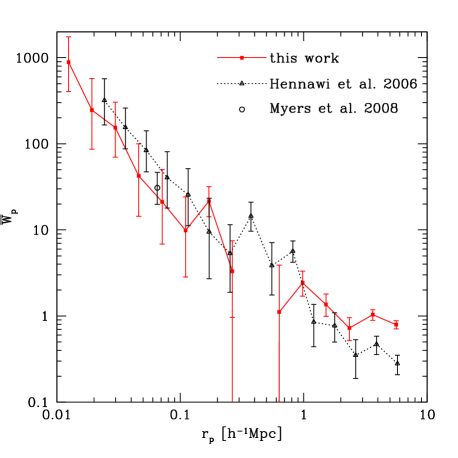
Figure 2: The measured projected correlation function $\bar{W}_{p}(r_{p})$ as a function of the comoving separation $r_{p}$, based on the binary quasar sample from the SQLS (filled squares). For comparison, previous small-scale clustering measurements by Hennawi et al. (2006) and Myers et al. (2008) are shown by filled triangles and open circle, respectively.

Figure 2 plots the measured projected correlation function, $\bar{W}_{p}$ with errors assuming the Poisson distribution. Note that the gap around $0.4h^{-1}{\rm Mpc}$ is due to the exclusion of $20^{\prime\prime}<\theta<55^{\prime\prime}$. We find that the correlation function rises steeply toward smaller scales down to $0.01h^{-1}{\rm Mpc}$, which basically confirms the finding of Hennawi et al. (2006) that the small-scale clustering amplitudes of quasars are high. However, the clustering amplitudes in our analysis appears to be systematically smaller than those of Hennawi et al. (2006). We ascribe this difference to the uncertainty associated with the completeness. We also plot the clustering measurement by Myers et al. (2008), who constructed a complete binary quasar sample only for a narrow separation range to make a robust clustering measurement. The result of Myers et al. (2008) is more consistent with our result, which supports the argument that our binary quasar sample is nearly complete. It is worth noting that there is a difference of $\bar{W}_{p}$ at $\theta>55^{\prime\prime}$ between our measurement and that of Hennawi et al. (2006). While the origin of the difference is not clear, we note that our measurement at $\theta>55^{\prime\prime}$ is in good agreement with clustering measurement of Ross et al. (2009), as we will see later.

3.2 Power-law Fit

We fit the measured correlation function with a single power-law of the form $\xi(r)=(r/r_{0})^{-\gamma}$, where $\xi(r)$ is the three-dimensional real-space correlation function. Such simple model is still very useful not only for quantifying the behavior of the correlation function for a wide separation range, but also for comparing correlation function measurements for different objects and redshifts.

Here we combine our small-scale clustering measurements with large-scale measurements by Ross et al. (2009) to constrain the correlation function parameters. More specifically, we simultaneously fit our measurements of $\bar{W}_{p}(r_{p})$ (Eq. 20) at $r_{p}<0.3h^{-1}{\rm Mpc}$ and $w_{p}(r_{p})$ (Eq. 22) measurements by Ross et al. (2009) at $r_{p}>0.3h^{-1}{\rm Mpc}$ with two parameters, $r_{0}$ and $\gamma$. Note that the fitting ranges of $r_{p}$ are chosen to avoid any overlap of these two data. Although the redshift range of the Ross et al. (2009) quasar sample, $0.3<z<2.2$, is slightly different from ours, we ignore this small difference throughout the paper. Note that we adopt the Poisson error for $\bar{W}_{p}(r_{p})$, whereas Ross et al. (2009) estimated the error on $w_{p}(r_{p})$ using the jackknife resampling. We ignore the difference because Ross et al. (2009) also showed that their jackknife errors are not very different from the Poisson estimate at the scale considered here. We summarize the calculation of $\bar{W}_{p}(r_{p})$ and $w_{p}(r_{p})$ for the power-law model in Appendix A.

The comparison of the best-fit power-law model with the data is shown in Figure 3. We find the best-fit values to $r_{0}=5.37_{-0.39}^{+0.32}h^{-1}{\rm Mpc}$ and $\gamma=1.92_{-0.05}^{+0.04}$. These are quite consistent with the best-fit parameter values of Ross et al. (2009), $r_{0}=5.45_{-0.45}^{+0.35}h^{-1}{\rm Mpc}$ and $\gamma=1.90_{-0.03}^{+0.04}$, which indicates that the measured small-scale clustering is quite consistent with the extrapolation of large-scale clustering measurements. Note that the reduced $\chi^{2}$ at the best-fit values is 1.64, indicating that the measured correlation function in fact deviates from a power-law, as is the case for the correlation function of galaxies (Zehavi et al., 2004). We also consider the case that the slope is fixed to $\gamma=2$, and find the best-fit correlation length for this case to $r_{0}=5.40_{-0.33}^{+0.31}h^{-1}{\rm Mpc}$.

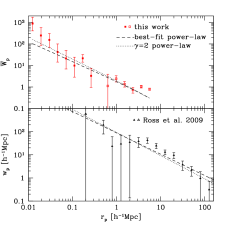
Figure 3: Power-law fit to the projected correlation functions. We show the result of the simultaneous fit to the projected correlation function $\bar{W}_{p}(r_{p})$ (upper panel) measured in this paper and the large-scale correlation function $w_{p}(r_{p})$ (lower panel) measured by Ross et al. (2009). Dashed lines are the best-fit power-law model with two parameters $r_{0}$ and $\gamma$, while dotted lines are the result of power-law fitting with a fixed slope $\gamma=2$. The data points shown in filled symbols indicate that they are used for the fitting.

4 Halo Model Interpretation

4.1 Model Description

The Halo Occupation Distribution (HOD) framework (Seljak, 2000; Peacock & Smith, 2000; Scoccimarro et al., 2001) provides more physical interpretation of the correlation function measurements. This model assumes numbers of objects in individual dark haloes as a function of halo masses, $\langle N(M)\rangle$, as well as how the objects are distributed within haloes. The technique has been used for the analysis of the quasar/AGN correlation function measurements to study quasar activities within a cosmological framework (Porciani et al., 2004; Miyaji et al., 2011; Krumpe et al., 2012; Richardson et al., 2012).

In the halo model description, we divide the power spectrum into two parts, the so-called one-halo and two-halo terms

$$P(k)=P_{\rm 1h}(k)+P_{\rm 2h}(k).$$ (6)

The projected correlation function can be obtained by (e.g., Cooray & Sheth, 2002)

$$w_{p}(r_{p})=\int_{0}^{\infty}\frac{kdk}{2\pi}P(k)J_{0}(kr_{p}),$$ (7)

where $J_{0}(x)$ is the zeroth-order Bessel function of the first kind.

The two-halo term is simply estimated as

$$P_{\rm 2h}(k)=b^{2}P_{\rm lin}(k),$$ (8)

where $b$ is the linear bias parameter which can be modelled as

$$b=\frac{1}{n_{q}}\int b_{\rm h}(M)\langle N(M)\rangle\frac{dn}{dM}dM,$$ (9)

$$n_{q}=\int\langle N(M)\rangle\frac{dn}{dM}dM,$$ (10)

where we adopt the halo mass function $dn/dM$ and the halo bias model $b_{\rm h}(M)$ of Sheth & Tormen (1999). The linear matter power spectrum $P_{\rm lin}(k)$ is computed using a fitting form of Eisenstein & Hu (1999) with the baryon density $\Omega_{b}=0.045$, the amplitude of fluctuations $\sigma_{8}=0.80$, and the slope of the initial power spectrum $n_{s}=0.963$. We model the mean number of quasars in each halo, $\langle N(M)\rangle$, by the following simple form

$$\langle N(M)\rangle=f_{N}\times\frac{1}{\sqrt{2\pi}\Delta_{m}}\exp\left[-\frac{\ln^{2}(M/M_{m})}{2\Delta_{m}^{2}}\right].$$ (11)

This functional form is motivated by Lidz et al. (2006) who investigated the luminosity dependence of quasar clustering and the quasar luminosity functions and concluded that quasars with a broad luminosity range reside in host haloes with a narrow range of masses. In addition, several observational works have shown that there is a deficit of quasar lying in massive clusters, at least at $z\la 1$ (e.g., Green et al., 2011; Farina et al., 2011; Harris, 2012), which also supports this HOD model. Our model is also consistent with a recent HOD analysis result of X-ray AGNs by Miyaji et al. (2011). Following the argument of Lidz et al. (2006), in this paper we fix $\Delta_{m}=0.75$, leading to a fairly narrow mass range of $\sim 2$ dex, although we confirmed that our conclusion is insensitive to the choice of $\Delta_{m}$. The normalization of Eq. (11), $f_{N}$, is calculated for each HOD parameter set by matching the number density of quasars to the observed one, $n_{q}\sim 1.35\times 10^{-6}h^{3}{\rm Mpc}^{-3}$ at the mean redshift of $z=1.40$ for our sample.

The one-halo term can be described as (Seljak, 2000)

$$P_{\rm 1h}(k)=\frac{1}{n_{q}^{2}}\int\langle N(N-1)\rangle u(k,M)^{p}\frac{dn}{dM}dM.$$ (12)

Here, $u(k,M)$ is the Fourier transform of the number density profile of quasars in a dark matter halo with mass $M$ which is normalized to unity at $k\to 0$. The parameter $p$ is basically determined by the fraction of quasars that reside in the centre of the halo. In this paper, we consider a simple model that assumes a constant “satellite fraction” $f_{\rm sat}$. This parameter is defined by the fraction of quasars that appears as satellites in dark matter haloes. Then the HOD of central and satellite components (see, e.g., Berlind & Weinberg, 2002; Kravtsov et al., 2004; Zheng et al., 2005) are described by $\langle N_{\rm cen}\rangle=(1-f_{\rm sat})\langle N(M)\rangle$ and $\langle N_{\rm sat}\rangle=f_{\rm sat}\langle N(M)\rangle$, respectively. We ignore the mass dependence of $f_{\rm sat}$, which is easily justified when we consider relatively narrow range of halo masses as assumed in this paper. Furthermore, we assume that the central quasar activity and the satellite activity are independent of each other. In this case, we can simplify the integral kernel as

$$\langle N(N-1)\rangle u(k,M)^{p}$$ (13)

$$\equiv 2\langle N_{\rm cen}N_{\rm sat}\rangle u(k,M)+\langle N_{\rm sat}(N_{\rm sat}-1)\rangle|u(k,M)|^{2}$$

$$=\left[2f_{\rm sat}(1-f_{\rm sat})u(k,M)+f_{\rm sat}^{2}|u(k,M)|^{2}\right]\langle N(M)\rangle^{2},$$

where we assumed Poisson statistics. In this model, neither the one-halo nor two-halo term depend on the normalization $f_{N}$ in Eq. (11).

For the number density profile of quasars in a dark matter halo, we employ the NFW profile (Navarro et al., 1995) with the concentration parameter $c_{\rm vir}$ of Bullock et al. (2001) or a Singular Isothermal Sphere (SIS) profile. Both the profiles are truncated at the virial radius of each dark matter halo.

4.2 Data Conversion: $\bar{W}_{p}$ to $w_{p}$

While our measurement of $\bar{W}_{p}(r_{p})$ enables direct comparisons with Hennawi et al. (2006), it is computationally more efficient to work on $w_{p}(r_{p})$ for the comparison of the HOD model with the data. Here we attempt to convert our measurements of $\bar{W}_{p}(r_{p})$ to $w_{p}(r_{p})$ adopting the following approximation. The conversion makes it easier to compare our results with other correlation function measurements.

We do so by multiplying the following approximated conversion factor to $\bar{W}_{p}(r_{p})$

$$\int_{z_{\rm min}}^{z_{\rm max}}dz\frac{dV_{c}}{dz}n(z)2v_{z}\times\frac{\bar{w}_{p}(r_{p})}{\bar{w}_{p}(r_{p},v_{\rm max})},$$ (14)

where

$$\bar{w}_{p}(r_{p},v_{\rm max}) \equiv \frac{1}{N}\int_{z_{\rm min}}^{z_{\rm max}}dz\frac{dV_{c}}{dz}n(z)$$ (15)

$$\times\int_{0}^{v_{z}}d\pi\xi(\sqrt{r_{p}^{2}+\pi^{2}},z),$$

and $\bar{w}_{p}(r_{p})\equiv\bar{w}_{p}(r_{p},v_{\rm max}\to\infty)$. The second term of Eq (14) is evaluated assuming that the real-space correlation function is a power-law with $r_{0}=5.37h^{-1}{\rm Mpc}$ and $\gamma=1.92$.

Table 2: Projected correlation functions $\bar{W}_{p}(r_{p})$ and $w_{p}(r_{p})$ measured in this paper. Note that $w_{p}(r_{p})$ in this table are approximated values computed by the method described in §4.2. Values in parentheses indicate measurement errors.

$r_{p}$	$\bar{W}_{p}(r_{p})$	$w_{p}(r_{p})$
($h^{-1}{\rm Mpc}$)		($h^{-1}{\rm Mpc}$)
0.012	888.748 (513.696)	42157.4 (24367.0)
0.019	246.645 (175.112)	11703.3 (8309.1)
0.030	154.087 (89.539)	7315.0 (4250.7)
0.046	42.409 (30.695)	2014.7 (1458.2)
0.071	21.161 (15.671)	1006.4(745.3)
0.110	9.850 (7.672)	469.2 (365.5)
0.171	21.545 (7.515)	1028.8 (358.9)
0.265	3.304 (2.485)	158.3( 119.1)
0.409	$\cdots$	$\cdots$
0.634	1.114 (1.495)	54.2 (72.7)
0.981	2.429 (0.731)	119.5 (36.0)
1.518	1.361 (0.373)	68.2 (18.7)
2.349	0.725 (0.206)	37.4 (10.6)
3.636	1.037 (0.145)	55.9 (7.8)
5.627	0.795 (0.088)	45.9 (5.1)

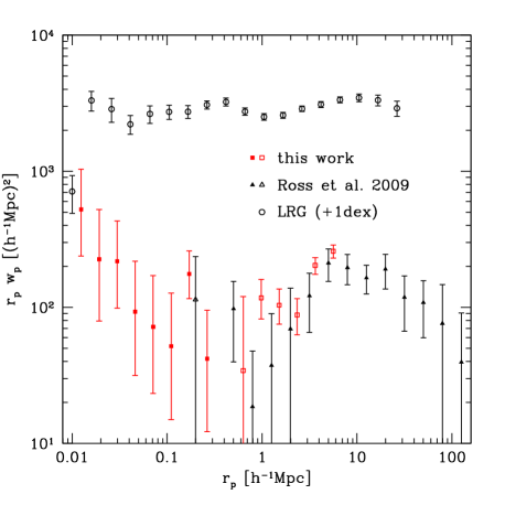
Figure 4: Projected correlation function $w_{p}(r_{p})$ of quasars from our measurement (squares) and and that of Ross et al. (2009) (triangles). For comparison, we also plot the projected correlation function of LRGs at $z\sim 0.3$ (open circles) measured by Masjedi et al. (2006) and Zehavi et al. (2005). Note that the LRG correlation function is shifted upward by 1 dex for illustrative purpose. The data points shown in filled symbols indicate that they are used for the fitting.

We show the estimated $w_{p}(r_{p})$ as well as the original projected correlation function in Table 2. We also plot $w_{p}(r_{p})$ from our measurements and that from Ross et al. (2009) in Figure 4. For comparison, we also show the correlation function of Luminous Red Galaxies (LRGs) at $z\sim 0.3$ measured by Masjedi et al. (2006) and Zehavi et al. (2005). We find that the overall shape of $w_{p}(r_{p})$ for quasars is quite similar to that for LRGs. Both the correlation functions show deviations from a power-law in a similar manner, which can be better fitted by a more general HOD model as we will see in §4.3. We however note a possible difference in the shapes of $w_{p}(r_{p})$ at the smallest separations of $r_{p}\sim 10h^{-1}{\rm kpc}$. The LRG correlation function appears to decrease significantly at the smallest bin, which is also suggested by the recent measurement of the satellite galaxy distribution around LRGs (Tal et al., 2012), whereas there is a hint of excess at the smallest separations in the quasar correlation function. The difference might be explained by different effects of direct interactions on quasars and galaxies.

4.3 Result of Fitting

Here we compare the HOD model predictions with measurements of $w_{p}(r_{p})$ derived in §4.2. For simplicity, calculations of $w_{p}(r_{p})$ with the HOD model are done at the mean redshift of our parent quasar samples of $z=1.40$. Our HOD model involves only two parameters, $M_{m}$ and $f_{\rm sat}$. Considering the fact that the two-halo term is independent of $f_{\rm sat}$ and that the data points of Ross et al. (2009) lie in the scale where the two-halo term is dominant, we first use the measurement of Ross et al. (2009) at $r_{p}>0.3h^{-1}{\rm Mpc}$ to fit $M_{m}$ only. The best-fit value is found to $M_{m}=1.33_{-0.32}^{+0.36}\times 10^{13}h^{-1}M_{\odot}$, and the resulting normalization is $f_{N}=7.6\times 10^{-3}$. This means that dark matter halos with the peak mass of $M=M_{m}$ harbour $\sim 4\times 10^{-3}$ quasars on the average. Figure 5 plots the best-fit $\langle N(M)\rangle$ and the host halo mass distribution $\langle N(M)\rangle dn/dM$. The latter which indicates the typical mass of host halo harboring quasars peaks at $\sim 3\times 10^{12}h^{-1}M_{\odot}$, which is consistent with previous measurements for optical quasars (e.g., Shen et al., 2007; Coil et al., 2007; Ross et al., 2009; Richardson et al., 2012). Next, we fit the small-scale measurements derived in this paper to constrain $f_{\rm sat}$ with a fixed peak mass in $\langle N(M)\rangle$, $M_{m}=1.33\times 10^{13}h^{-1}M_{\odot}$.

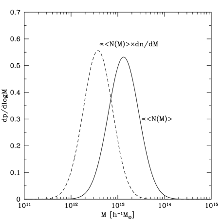
Figure 5: The best-fit HOD model $\langle N(M)\rangle$ (solid) and the host halo mass distribution $\langle N(M)\rangle dn/dM$ (dashed). Both curves are normalized so that it becomes unity when integrated over $d\log M$.

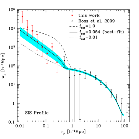
Figure 6: HOD model predictions of the projected correlation function $w_{p}(r_{p})$ for three different satellite fraction, $f_{\rm sat}=1$ (dashed), $0.054$ (solid), and $0.01$ (dotted). An SIS profile is assumed for the radial number density profile of satellites. The peak mass in $\langle N(M)\rangle$, $M_{m}$ in Eq. (11), is fixed to the best-fit value. The shaded region around the best-fit model represents $1\sigma$ range.

We find that $f_{\rm sat}=0.054_{-0.016}^{+0.017}$ for an SIS profile and $f_{\rm sat}=0.048_{-0.015}^{+0.016}$ for an NFW profile. Combining the $\chi^{2}$ of the large-scale and small-scale fitting, the reduced $\chi^{2}$s for the best-fit parameters are 0.83 for the SIS profile and 0.89 for the NFW profile, which are significantly better than the reduced $\chi^{2}$ of 1.64 for the power-law fit shown in §3.2, despite the same number of free parameters these models contain. Figure 6 illustrates how the small-scale clustering measurements presented in this paper constrain $f_{\rm sat}$. Basically $f_{\rm sat}$ controls the amplitude of the one-halo term such that larger satellite fractions predict larger small-scale clustering amplitudes.

Figure 7 compares our best-fit HOD models for SIS and NFW profiles with the measurements. Except for a few points at the smallest scales, our HOD model reproduces the global feature of the measured correlation function very well. At the smallest scale around $\sim 10h^{-1}{\rm kpc}$, the difference of assumed number density profile of quasars in a halo becomes prominent as expected, although even the steep SIS profile fails to reproduce the clustering amplitude at these scales. Hence, we also consider the case of an NFW profile with the concentration parameter value enhanced by a factor of 10 compared with our fiducial model (Bullock et al., 2001). This enhanced concentration model predicts $c_{\rm vir}\sim 30$ for haloes with mass $M=M_{m}$ at $z=1.4$. The result shown in Figure 7 indicates that this high-concentration model better reproduces the strong small-scale clustering found in the measurements.

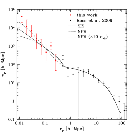
Figure 7: Comparisons of the best-fit HOD model predictions for the projected correlation function assuming SIS (solid) and NFW (dotted) profiles with the measurements. The dashed line shows the HOD model assuming an NFW profile, but with 10 times larger concentration parameter than the fiducial Bullock et al. (2001) model.

5 Conclusion

We have measured the small-scale correlation function of low-redshift ($0.6<z<2.2$) quasars using a new sample of 26 spectroscopically confirmed binary quasars from the SQLS. The angular separation range of $1^{\prime\prime}<\theta<20^{\prime\prime}$ for the binary quasar sample allows us to measure the quasar auto-correlation function from the projected comoving separation $r_{p}\sim 200h^{-1}{\rm kpc}$ down to $r_{p}\sim 10h^{-1}{\rm kpc}$. To do so, we have assumed that our binary quasar sample is complete within a specified range of redshifts and angular separations, which is based on careful selections and extensive follow-up observations of the SQLS in order to construct a complete gravitational lens sample. We have found that the correlation function rises steeply toward smaller separations. Our result is in reasonable agreement with earlier result by Hennawi et al. (2006), in which large corrections of sample incompleteness has been applied to measure small-scale clustering signals. While the measured small-scale clustering in our analysis appears to be slightly smaller than the result of Hennawi et al. (2006), we note that our result is more consistent with the clustering amplitude measurement within a narrow separation range presented by Myers et al. (2008) based on a complete binary quasar sample. By combining our measurements with the large-scale correlation function obtained by Ross et al. (2009), we have fitted the correlation functions for a wide range of $0.01h^{-1}{\rm Mpc}\la r_{p}\la 10h^{-1}{\rm Mpc}$ by a power-law $\xi(r)=(r/r_{0})^{-\gamma}$, and found the best-fit values to $r_{0}=5.37_{-0.39}^{+0.32}h^{-1}{\rm Mpc}$ and $\gamma=1.92_{-0.05}^{+0.04}$. The measured correlation function can be described reasonably well by this single power-law model over 4 order of magnitudes in $r_{p}$.

We have interpreted the measured quasar correlation function within the framework of the HOD. In particular, we have proposed a simple HOD model that assumes a constant satellite fraction $f_{\rm sat}$, which is a reasonable assumption when the average number of quasars in haloes with mass $M$, $\langle N(M)\rangle$, becomes large within relatively narrow range in masses. Using this model, we have shown how the small-scale clustering can be used to constrain $f_{\rm sat}$. The best-fit satellite fraction of our quasar sample is $f_{\rm sat}=0.054_{-0.016}^{+0.017}$ for an SIS profile and $f_{\rm sat}=0.048_{-0.015}^{+0.016}$ for an NFW profile. The HOD model reproduces the measured correlation function quite well, except at the smallest separations of $r_{p}\sim 10h^{-1}{\rm kpc}$ where the model slightly under-predicts clustering signals even if we assume the steep SIS profile for the spatial distribution of satellite components. We find that even steeper profiles, such as an NFW profile with the concentration parameter of $c_{\rm vir}\ga 30$, are needed to explain the measured clustering amplitudes at the smallest scale. Recent numerical simulations of low-luminosity AGN also suggest that radial profile of AGN inside haloes is much steeper than the normal NFW profile (DeGraf et al., 2011; Chatterjee et al., 2012). Such excess clustering at the smallest separations, as well as possible different behaviors between quasar and LRG correlation functions at those scales (see Watson et al., 2010, for a discussion on the radial profile of LRGs from HOD modelling), might be due to an enhanced quasar activity by mergers. Direct high-resolution imaging of host galaxies for these very small-separation binary quasars might be helpful for testing this hypothesis.

When we almost finished this paper, we found that Richardson et al. (2012) conducted similar HOD analysis of quasar clustering to constrain the satellite fraction, using small-scale clustering measurements of Hennawi et al. (2006). However, their best-fit satellite fraction of $f_{\rm sat}=(7.4\pm 1.4)\times 10^{-4}$ for quasars at $z\sim 1.4$ appear to be significantly smaller than our result. This discrepancy is explained by different forms of HOD modelling adopted in both papers. Their $\langle N(M)\rangle$ extends toward the mass scale of massive clusters where satellite components dominate the mean number of quasars, whereas in our HOD model we have assumed a deficit of quasars in very massive clusters. We confirmed that their best-fit HOD model indeed predicts significantly smaller $f_{\rm sat}$ than our result. Also note that we have assumed that the quasar activities of the central and the satellite quasars are independent of each other, which means that quasars can be satellites even if the central object is not a quasar. When there exists a strong central-satellite correlation such that haloes are allowed to host satellite quasars only if the central galaxy is also a quasar, we expect that smaller $f_{\rm sat}$ can recover the small-scale clustering of quasar pairs. In this sense, our best-fit $f_{\rm sat}$ value may be considered as an upper limit. Detailed observation of the environment of (binary) quasars or dynamical analysis of quasar pairs might provide more direct information on the mass of host haloes of quasars and on the location of quasars in the host haloes (e.g., Fukugita et al., 2004; Serber et al., 2006; Boris et al., 2007; Strand et al., 2008; Green et al., 2011; Farina et al., 2011; Harris, 2012).

Appendix A Power-Law Model Calculation

We derive the relations between the power-law model of $\xi(r)=(r/r_{0})^{-\gamma}$ and the projected correlation functions $\bar{W}_{p}(r_{p})$ and $w_{p}(r_{p})$.

The projected correlation function, $\bar{W}_{p}$, can be interpreted as an average over the parent quasar sample

$$\bar{W}_{p}(r_{p,\rm min},r_{p,\rm max})=\frac{1}{N_{\rm QSO}}\sum_{j}^{N_{\rm QSO}}\bar{W}_{p}(z_{j},r_{p,\rm min},r_{p,\rm max}),$$ (16)

where $\bar{W}_{p}(z_{j},r_{p,\rm min},r_{p,\rm max})$ is computed as

$$\bar{W}_{p}(z,r_{p,\rm min},r_{p,\rm max})=\frac{\int_{-v_{z}}^{v_{z}}d\pi\int_{r_{p,\rm min}}^{r_{p,\rm max}}dr_{p}2\pi r_{p}\xi(r_{p},\pi,z)}{V_{\rm shell}(z,r_{p,\rm min},r_{p,\rm max})},$$ (17)

with $\xi(r_{p},\pi)$ being the anisotropic redshift-space correlation function and $v_{z}\equiv v_{\rm max}(1+z)/H(z)$ (Hennawi et al., 2006). In this paper, we employ the following approximated expressions in order to speed up the computation:

$$\bar{W}_{p}(r_{p})\sim\frac{1}{N}\int_{z_{\rm min}}^{z_{\rm max}}dz\frac{dV_{c}}{dz}n(z)\frac{1}{v_{z}}\int_{0}^{v_{z}}d\pi\xi(\sqrt{r_{p}^{2}+\pi^{2}},z),$$ (18)

where $\xi(r,z)$ is the isotropic real-space correlation function, $z_{\rm min}=0.6$ and $z_{\rm max}=2.2$ are the minimum and maximum of the redshift range, $r_{p}$ is set to $(r_{p,\rm min}+r_{p,\rm max})/2$, $n(z)$ is the comoving number density of quasars (brighter than $i=19.1$ for our case), and

$$N=\int_{z_{\rm min}}^{z_{\rm max}}dz\frac{dV_{c}}{dz}n(z).$$ (19)

When $\xi(r)$ is described by a single power-law of $\xi(r)=(r/r_{0})^{-\gamma}$, Eq (18) can be simplified as

$$\bar{W}_{p}(r_{p}) \sim \frac{1}{N}\int_{z_{\rm min}}^{z_{\rm max}}dz\frac{dV_{c}}{dz}n(z)$$ (20)

$$\times\left(\frac{r_{0}}{r_{p}}\right)^{\gamma}\ _{2}F_{1}\left(\frac{1}{2},\frac{\gamma}{2},\frac{3}{2},-\frac{v_{z}^{2}}{r_{p}^{2}}\right),$$

where ${}_{2}F_{1}(a,b,c;x)$ is the Gauss’ hypergeometric function.

On the other hand, the projected correlation function $w_{p}(r_{p})$, which is more commonly used, is defined by

$$w_{p}(r_{p})=2\int_{0}^{\infty}d\pi\xi(\sqrt{r_{p}^{2}+\pi^{2}}).$$ (21)

Again, when $\xi(r)$ is described by a single power-law of $\xi(r)=(r/r_{0})^{-\gamma}$ with $\gamma>1$, $w_{p}(r_{p})$ can be computed as

$$w_{p}(r_{p})=\frac{r_{0}^{\gamma}\sqrt{\pi}\Gamma((\gamma-1)/2)}{\Gamma(\gamma/2)}r_{p}^{1-\gamma},$$ (22)

where $\Gamma(x)$ is the Gamma function.

References

- Berlind & Weinberg (2002) Berlind A. A., Weinberg D. H., 2002, ApJ, 575, 587
- Boris et al. (2007) Boris N. V., Sodré L. Jr., Cypriano E. S., Santos W. A., Mendes de Oliveira C., West M., 2007, ApJ, 666, 747
- Bullock et al. (2001) Bullock J. S., Kolatt T. S., Sigad Y., Somerville Kravtsov R. S., A. V., Klypin A. A., Primack J. R., Dekel A., 2001, MNRAS, 321, 559
- Coil et al. (2007) Coil A. L., Hennawi J. F., Newman J. A., Cooper M. C., Davis M., 2007, ApJ, 654, 115
- Cooray & Sheth (2002) Cooray A., Sheth R., 2002, PhR, 372, 1
- Chatterjee et al. (2012) Chatterjee S., Degraf C., Richardson J., Zheng Z., Nagai D., Di Matteo T., 2012, MNRAS, 419, 2657
- Croom et al. (2005) Croom S. M., et al., 2005, MNRAS, 356, 415
- Croom et al. (2009) Croom S. M., et al., 2009, MNRAS, 399, 1755
- DeGraf et al. (2011) Degraf C., Oborski M., Di Matteo T., Chatterjee S., Nagai D., Richardson J., Zheng Z., 2011, MNRAS, 416, 1591
- Di Matteo et al. (2005) Di Matteo T., Springel V., Hernquist L., 2005, Natur, 433, 604
- Eisenstein & Hu (1999) Eisenstein D.J., Hu W., 1999, ApJ, 511, 5
- Ellison et al. (2011) Ellison S. L., Patton D. R., Mendel J. T., Scudder J. M., 2011, MNRAS, 418, 2043
- Farina et al. (2011) Farina E. P., Falomo R., Treves A., 2011, MNRAS, 415, 3163
- Ferrarese & Merritt (2000) Ferrarese L., Merritt D., 2000, ApJ, 539, L9
- Fukugita et al. (2004) Fukugita M., Nakamura O., Schneider D. P., Doi M., Kashikawa N., 2004, ApJ, 603, L65
- Gebhardt et al. (2000) Gebhardt K., et al., 2000, ApJ, 539, L13
- Green et al. (2010) Green P. J., Myers A. D., Barkhouse W. A., Mulchaey J. S., Bennert V. N., Cox T. J., Aldcroft T. L., 2010, ApJ, 710, 1578
- Green et al. (2011) Green P. J., Myers A. D., Barkhouse W. A., Aldcroft T. L., Trichas M., Richards G. T., Ruiz Á., Hopkins P. F., 2011, ApJ, 743, 81
- Harris (2012) Harris K. A., 2012, arXiv:1201.5746
- Hennawi et al. (2006) Hennawi J. F., et al., 2006, AJ, 131, 1
- Hennawi et al. (2010) Hennawi J. F., et al., 2010, ApJ, 719, 1672
- Hopkins et al. (2008) Hopkins P. F., Hernquist L., Cox T. J., Kereš D., 2008, ApJS, 175, 356
- Inada et al. (2008) Inada N., et al., 2008, AJ, 135, 496
- Inada et al. (2010) Inada N., et al., 2010, AJ, 140, 403
- Inada et al. (2012) Inada N., et al., 2012, AJ, 143, 119
- Koss et al. (2010) Koss M., Mushotzky R., Veilleux S., Winter L., 2010, ApJ, 716, L125
- Kravtsov et al. (2004) Kravtsov A. V., Berlind A. A., Wechsler R. H., Klypin A. A., Gottlöber S., Allgood B., Primack J. R., 2004, ApJ, 609, 35
- Krumpe et al. (2012) Krumpe M., Miyaji T., Coil A. L., Aceves H., 2012, ApJ, 746, 1
- Lidz et al. (2006) Lidz A., Hopkins P. F., Cox T. J., Hernquist L., Robertson B., 2006, ApJ, 641, 41
- Liu et al. (2012) Liu X., Shen Y., Strauss M. A., 2012, ApJ, 745, 94
- Magorrian et al. (1998) Magorrian J., et al., 1998, AJ, 115, 2285
- Masjedi et al. (2006) Masjedi M., et al., 2006, ApJ, 644, 54
- Michel & Stoitsov (2008) Michel N., Stoitsov M. V., 2008, CPC, 178, 535
- Miyaji et al. (2011) Miyaji T., Krumpe M., Coil A. L., Aceves H., 2011, ApJ, 726, 83
- Myers et al. (2006) Myers A. D., et al., 2006, ApJ, 638, 622
- Myers et al. (2007) Myers A. D., Brunner R. J., Richards G. T., Nichol R. C., Schneider D. P., Bahcall N. A., 2007, ApJ, 658, 99
- Myers et al. (2008) Myers A. D., Richards G. T., Brunner R. J., Schneider D. P., Strand N. E., Hall P. B., Blomquist J. A., York D. G., 2008, ApJ, 678, 635
- Navarro et al. (1995) Navarro J. F., Frenk C. S., White S. D. M., 1995, MNRAS, 275, 56
- Oguri et al. (2006) Oguri M., et al., 2006, AJ, 132, 999
- Oguri et al. (2008) Oguri M., et al., 2008, AJ, 135, 512
- Oguri et al. (2012) Oguri M., et al., 2012, AJ, 143, 120
- Padmanabhan et al. (2009) Padmanabhan N., White M., Norberg P., Porciani C., 2009, MNRAS, 397, 1862
- Peacock & Smith (2000) Peacock J. A., Smith R. E., 2000, MNRAS, 318, 1144
- Pindor et al. (2006) Pindor B., et al., 2006, AJ, 131, 41
- Porciani & Norberg (2006) Porciani C., Norberg P., 2006, MNRAS, 371, 1824
- Porciani et al. (2004) Porciani C., Magliocchetti M., Norberg P., 2004, MNRAS, 355, 1010
- Richards et al. (2006) Richards T. G., et al., 2006, AJ, 131, 2766
- Richardson et al. (2012) Richardson J., Zheng Z., Chatterjee S., Nagai D., Shen Y., 2012, ApJ, submitted (arXiv:1203.4570)
- Ross et al. (2009) Ross N. P., et al., 2009, ApJ, 697, 1634
- Schneider et al. (2010) Schneider D. P., et al., 2010, AJ, 139, 2360
- Scoccimarro et al. (2001) Scoccimarro R., Sheth R. K., Hui L., Jain B., 2001, ApJ, 546, 20
- Seljak (2000) Seljak U., 2000, MNRAS, 318, 203
- Serber et al. (2006) Serber W., Bahcall N., Ménard B., Richards T. G., 2006, ApJ, 643, 68
- Shen et al. (2007) Shen Y., et al., 2007, AJ, 133, 2222
- Shen et al. (2009) Shen Y., et al., 2009, ApJ, 697, 1656
- Shen et al. (2010) Shen Y., et al., 2010, ApJ, 719, 1693
- Sheth & Tormen (1999) Sheth R.K., Tormen G., 1999, MNRAS, 308, 119
- Silverman et al. (2011) Silverman J. D., et al., 2011, ApJ, 743, 2
- Strand et al. (2008) Strand N. E., Brunner R. J., Myers A. D., 2008, ApJ, 688, 180
- Tal et al. (2012) Tal T., Wake D. A., van Dokkum P. G., 2012, ApJL, submitted (arXiv:1201.5114)
- Tremaine et al. (2002) Tremaine S., et al., 2002, ApJ, 574, 740
- Watson et al. (2010) Watson D. F., Berlind A. A., McBride C. K., Masjedi M., 2010, ApJ, 709, 115
- White et al. (2012) White M., et al. 2012, arXiv:1203.5306
- Zehavi et al. (2004) Zehavi I., et al., 2004, ApJ, 608, 16
- Zehavi et al. (2005) Zehavi I., et al., 2005, ApJ, 621, 22
- Zheng et al. (2005) Zheng Z., et al., 2005, ApJ, 633, 791