Power Control in Multi-Layer Cellular Networks

Abstract

We investigate the possible performance gains of power control in multi-layer cellular systems where microcells and picocells are distributed within macrocells. Although multi-layers in cellular networks help increase system capacity and coverage, and can reduce total energy consumption; they cause interference, reducing the performance of the network. Therefore, downlink transmit power levels of multi-layer hierarchical cellular networks need to be controlled in order to fully exploit their benefits. In this work, we present an analytical derivation to determine optimum power levels for two-layer cellular networks and generalize our solution to multi-layer cellular networks. We also simulate our results in a typical multi-layer network setup and observe significant power savings compared to single-layer cellular networks.

I Introduction

Power savings in cellular networks are not only going to reduce operational expenses of operators but in addition, they will significantly impact global carbon dioxide emissions. It has been estimated that $2\%$ of global energy consumption is through information and communication technologies [1]. By the increase in the offered data rates in the new standards such as Long Term Evolution (LTE) and Worldwide Interoperability for Microwave Access (WiMAX), and expected increase in subscribed users, it is predicted that the power consumption of telecommunications and mobile communications in particular, will triple in the next decade [2, 3]. Approximately $60$-$80\%$ of the total power consumed in mobile communications is dissipated in the base stations, mainly through radio-frequency (RF) conversion, power amplification and site cooling processes [3, 4].

Application of multi-layer hierarchical cellular networks is proposed in upcoming standards such as LTE and LTE-Advanced to overcome the increasing demand in data rate and power [5, 6]. Several low power base stations such as microcells and picocells can be distributed within a larger high power base station cell, namely the macrocell. Hence, significant power savings are possible, high traffic loads can be passed onto lower layers where high-rate low-power transmission is possible, and any cell coverage problems such as shadowing effects caused by buildings can be resolved. Also, depending on the mobility pattern of users, coverage and excess handover traffic issues can be eliminated. In addition, higher data rates can be provided with careful network planning.

In this article, we investigate the deployment of two-layer hierarchical networks and consider high-power macrocells overlaid with low-power microcell systems, providing service within the same cell. We present an analytical solution to determine optimum power levels in these two-layer cellular systems. In cases where channel conditions between microcells and users are superior compared to macrocell base stations and users, macrocell base stations can switch to a sleep mode and let microcells transmit and receive data. This will provide significant power savings in total energy consumption of the system, and at the same time, deliver the same data rates to the users. We also generalize this analytical solution to determine the optimum power levels in multi-layer systems such as the one where macrocells, microcells and picocells coexist. For cases where the optimal solution exceeds permissible maximum power levels, we use another approach proposed by Raman et al. that uses linear programming (LP) to determine the best solution given maximum power level constraints of each base station [7]. We also show achievable power savings when multi-layers are deployed in the system through a simple simulation setup.

In Section II, the system models for single-layer and two-layer cellular networks are introduced and in Section III, we present our analytical solution to determine optimal power levels of both systems and generalize our solution to multi-layer cellular systems. We also investigate the necessary conditions for the existence of the proposed solutions. In Section IV, we include maximum power levels of each layer to the problem, and using these constraints, we explain how to update base station power levels using the LP approach in [7]. We explain our simulation setup and its parameters in Section V and show the power savings for a two-layer architecture when compared to a single-layer system. We conclude the paper with comments on the possible gains that can be achieved with the deployment of multiple layers in cellular networks.

II System Model

In this section, we present system models for both single-layer and two-layer cellular networks. A single-layer network constitutes a reference scenario where we compare the gains with respect to two-layer networks. To that end, we follow a simulation setup similar to [7] and consider a $19$-cell hexagonal layout seen in Figure 1. In each cell, we locate a base station tower at the center of the hexagon and deploy three sector antennas, each covering $120^{o}$ within the cell. To mitigate the edge effects, the wrap-around technique is employed [5]. Furthermore, we assume that all base stations in the system share the same resource that can be either the same time slot, same frequency channel, same spreading code or same time-frequency resource block as in LTE.

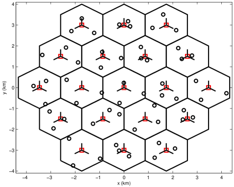
Figure 1: Single-layer network layout with $19$ hexagonal cells. Every cell has three-sector $120^{o}$ directional antennas positioned at the center of the cell. Each sector has one randomly placed user. Squares and circles depict macrocell base stations and users, respectively.

Users in the system are placed randomly within the cells one-by-one such that there is only one user in each sector as in [7]. The condition that we emphasize is that the generated user within each sector has to have the highest received signal strength from its associated base station. If this condition is not satisfied and the user needs to be handed over to the neighboring base station, we discard the user and generate another one. In total, we consider $57$ base stations and $57$ users in the system.

The first transmission is the learning phase for the channel conditions in the system. All base stations send the same predefined power level which we assumed as $5$ W. Assuming perfect feedback, the central processor obtains all the channel gains affecting every user. Then, the central processor discards a predetermined number of users and considers them in outage so that a common rate can be provided to the remaining users. The user discarding procedure is based on the path loss criteria and the users with the worst channel conditions are discarded. In the power control step, the optimum power levels are calculated using the analytical solution presented in the next section. The total transmit power in the system after the power control step forms the baseline system. We compare this value to the total transmit power in the two-layer cellular system after power control step for a fair comparison.

The two-layer cellular network includes additional microcell overlay on top of the macrocell structure included in the baseline system. We follow the simulation setup described in [8, 5] for the microcell deployment in urban areas and place microcell base stations on every other street on the Manhattan grid where each block in the grid is $200$ m, each street is $30$ m wide and microcells are deployed with omnidirectional antennas. Figure 2 depicts our two-layer cellular system layout where high-power macrocells and low-power microcells are deployed in the same area. User placement methodology is the same as in single-layer networks that each user is distributed randomly within each sector such that users have the highest signal strength within the cell they are associated with.

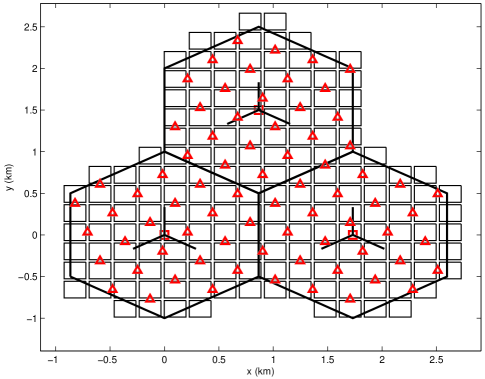
Figure 2: Two-layer hierarchical network layout with $19$ hexagonal cells overlaid with $467$ microcell base stations to model urban areas. Every cell includes 3-sector macrocell base stations placed in the center and depending on the geometry, $24-25$ microcells with omnidirectional antennas are deployed in Manhattan grids. Squares and triangles depict macrocell and microcell base stations, respectively, and only $3$ cells are shown for clarity.

The first transmission is devoted to a learning phase for the channel conditions in the system as it was for the single-layer network. Using the feedback from every user, the central processor forms the channel matrix of the system for both layers in the system. Here, note that the channel matrix is an augmented channel matrix which now includes the channel gain and path loss values for both macrocell and microcell layers. Based on the channel matrix, base station power levels for the two-layer cellular system are updated. For those cases where the channel conditions between users and microcell base stations are better than the macrocell base stations, those macrocell base stations do not transmit and switch to micro a sleep mode and let microcell base stations transmit. In the sequel, this total transmit power value after the power control step, including the sum of both layers is compared with the baseline system to quantify the gains of microcell deployment.

In the next section, we describe the analytical framework for the power control process in single-layer, two-layer and multi-layer cellular networks and comment on the necessary conditions for the existence of the solutions.

III Power Control

III-A Single-Layer System

In the single layer system, we only consider macrocells in the system and we are interested in power savings in the downlink since most of the power is dissipated in the base stations. The total power transmitted in this single-layer system constitutes our baseline case for comparison. We start our derivations by identifying the signal-to-interference-plus-noise-ratio (SINR) for user $i$ and write it as

$$\gamma_{i}=\frac{g_{ii}p_{i}}{\sum\limits_{j\neq i}g_{ij}p_{j}+\sigma_{i}^{2}}$$ (1)

where $p_{i}$ denotes the transmit power of $i$th base station and $g_{ij}$ includes the path loss and shadowing observed by user $i$ when base station $j$ transmits, $\sigma_{i}^{2}$ denotes the noise. When we rearrange the terms above and divide by $g_{ii}$, one would obtain

$$p_{i}=\gamma_{i}\sum\limits_{j\neq i}\frac{g_{ij}}{g_{ii}}p_{j}+\gamma_{i}\frac{\sigma_{i}^{2}}{g_{ii}}.$$ (2)

In vector-matrix form, the above equation can be written to include all users as follows

$$\textbf{p}=\textbf{F}\textbf{p}+\textbf{u}$$ (3)

where $u_{i}=\gamma_{i}\sigma_{i}^{2}/g_{ii}$ and

F $$=\begin{cases}\gamma_{i}g_{ij}/g_{ii}&\text{if }j\neq i\\ 0&\text{if }j=i\end{cases}$$

and we will refer to F as the normalized channel gain matrix for single-layer systems since it includes channel gains between every user and every base station. In F, except for the diagonal entries, the entries are normalized by the channel gain between the user and its associated base station. We can express the optimal solution by the vector $\textbf{p}^{*}$, that minimizes the total power in the single layer system as

$$\textbf{p}^{*}=(\textbf{I}_{N}-\textbf{F})^{-1}\textbf{u}$$ (4)

where $\textbf{I}_{N}$ is an $N\times N$ identity matrix. There are several comments to make about this solution. First, the normalized channel gain matrix is a nonnegative matrix since all its entries denote the channel gain values and these are always non-negative. Second, we assume each of these entries as realizations of the underlying stochastic processes, namely they are all random path loss variables, such that each channel gain in the system is determined independently and hence, F becomes a full-rank matrix. An important remark is that one seeks a nonnegativity constraint on the downlink transmit power levels of the base stations. Since u is always nonnegative, one needs to question the existence and the nonnegativity of $(\textbf{I}_{N}-\textbf{F})^{-1}$ for a feasible power level vector solution, $\textbf{p}^{*}$.

In order to determine the existence and the nonnegativity of the vector $\textbf{p}^{*}$, we apply the Perron-Frobenious theorem [9]. This theorem seeks the irreducibility of a matrix, therefore, one needs to check if F is an irreducible matrix or not. Following the same argument in [10], one sees that F would be reducible if and only if there exists more than one $0$ element on one row. Since we include the channel gains of every base station to every user using the wrap-around technique, we can conclude that F is irreducible. One direct result of the Perron-Frobenious theorem is that for an irreducible nonnegative matrix F, there always exists a positive real eigenvalue $\lambda^{*}$ of F and its associated eigenvector where $\lambda^{*}=\max\{\lambda\}_{i=1}^{N}=\rho(\textbf{F})$, is namely the spectral radius of F, and every component of its associated eigenvector is nonnegative [9]. Keeping these results in mind, one can rewrite (4) such that

$$\textbf{p}^{*}=(\textbf{I}_{N}-\textbf{F})^{-1}\textbf{u}=\frac{1}{1-\rho(\textbf{F})}\textbf{u}\geq\textbf{0}$$ (5)

and for the convergence of this solution we seek that the spectral radius of F needs to be less than 1, $\rho(\textbf{F})<1$. Here, we note that in previous works lead by Zander et al., this condition was already identified in [11, 13, 10, 12, 14, 15].

A major drawback of this approach is that it is a centralized solution. It is impractical for a central processor to have the perfect knowledge of all path loss values for all users in the system and determine the appropriate power levels for every user and send back the power levels to the associated base stations in a reasonable time. Therefore, several distributed solutions are proposed where each base station can iterate and adjust its power level using only the local acquired information without the need for a global central processor [13, 12, 14]. One distributed power solution is proposed by Foschini and Mijalcic where each base station updates its power level using the following rule [12]

$$p_{i}^{n+1}=\frac{\gamma_{i}}{g_{ii}}\left(\sum\limits_{j\neq i}g_{ij}p_{j}^{n}+\sigma_{i}^{2}\right)$$ (6)

where $p_{i}^{n}$ denotes the power level at base station $i$ at $n$th iteration. In vector-matrix form, the power update rule can be written as

$$\textbf{p}^{n+1}=\textbf{F}\textbf{p}^{n}+\textbf{u}$$ (7)

where $\textbf{p}^{n}$ denotes the vector of macrocell transmit power levels at $n$th iteration, and F and u are as defined above. Note that, in [12] it has been shown that for any initial power levels, using the above update rule, base station power levels converge to the optimal solution after several iterations.

III-B Two-Layer System

For the two-layer system, we consider both macrocell and microcell base stations and every user in the system experiences interference from both layers. The SINR at user $i$ can be written as

$$\gamma_{i}=\frac{g_{ii}p_{i}+h_{ii}q_{i}}{\sum_{j\neq i}\left(g_{ij}p_{j}+h_{ij}q_{j}\right)+\sigma_{i}^{2}}$$ (8)

where $p_{i}$ denotes the power transmitted from $i$th macrocell base station and $q_{i}$ is the transmit power of microcell base station $i$. The downlink channel coefficients for the path from macrocell base station $j$ to user $i$ is denoted by $g_{ij}$ and for microcell $j$ to user $i$ is shown by $h_{ij}$. The noise at receiver $i$ is represented as $\sigma_{i}^{2}$. Using these, the above equation can be further simplified as the following when we rearrange terms and divide every term by $g_{ii}$

$$p_{i}+\frac{h_{ii}}{g_{ii}}q_{i}=\gamma_{i}\sum_{j\neq i}\left(\frac{g_{ij}}{g_{ii}}p_{j}+\frac{h_{ij}}{g_{ii}}q_{j}\right)+\gamma_{i}\frac{\sigma_{i}^{2}}{g_{ii}}.$$

One can rewrite the above equation in vector-matrix form as

$$\underbrace{\left[\textbf{I}_{N}|\textbf{C}_{N\times N}\right]}_{\textbf{A}_{N\times 2N}}\underbrace{\left[\begin{array}[]{c}\textbf{p}\\ \textbf{q}\end{array}\right]}_{\textbf{x}_{2N\times 1}}=\underbrace{\left[\textbf{F}_{N\times N}|\textbf{G}_{N\times N}\right]}_{\textbf{B}_{N\times 2N}}\underbrace{\left[\begin{array}[]{c}\textbf{p}\\ \textbf{q}\end{array}\right]}_{\textbf{x}_{2N\times 1}}+\underbrace{\left[\begin{array}[]{c}\gamma_{1}\frac{\sigma_{1}^{2}}{g_{11}}\\ \vdots\\ \gamma_{N}\frac{\sigma_{N}^{2}}{g_{NN}}\end{array}\right]}_{\textbf{u}_{N\times 1}}$$ (16)

where $N$ denotes the number of users in the system, $\textbf{I}_{N}$ is an $N\times N$ identity matrix and C and G matrices are as shown below

C $$=\begin{cases}\frac{h_{ii}}{g_{ii}}&\text{if }j=i\\ 0&\text{if }j\neq i\end{cases},\textbf{G}=\begin{cases}\gamma_{i}\frac{h_{ij}}{g_{ii}}&\text{if }j\neq i\\ 0&\text{if }j=i.\end{cases}$$ (17)

We refer to H as the normalized channel gain matrix for microcell layer where the normalization is carried out with respect to macrocell layer path loss values, $g_{ii}$.

For the analytical solution for the two-layer system, one seeks to solve $\textbf{A}\textbf{x}=\textbf{B}\textbf{x}+\textbf{u}$. Rearranging the terms on each side, the problem can be restated as

$$\textbf{A}\left(\textbf{I}_{2N}-\widetilde{\textbf{B}}\right)\textbf{x}=\textbf{u}$$ (18)

where $\textbf{B}=\textbf{A}\widetilde{\textbf{B}}$ and $\widetilde{\textbf{B}}$ is such that $\widetilde{\textbf{B}}=\textbf{A}^{-1}\textbf{B}$. Also, $\textbf{A}^{-1}$ denotes the adjoint matrix of the rectangular matrix A. Then, the optimal solution for two-layer cellular system becomes

$$\textbf{x}^{*}=(\textbf{I}_{2N}-\widetilde{\textbf{B}})^{-1}\textbf{A}^{-1}\textbf{u}.$$ (19)

Let us analyze the existence and nonnegativity of the optimal solution vector, $\textbf{x}^{*}$. Following a similar analysis as in the single-layer case, given that $\widetilde{\textbf{B}}$ is nonnegative and irreducible, we can apply the Perron-Frobenious theorem and see that there always exists a componentwise nonnegative power vector $\textbf{x}^{*}$ given that the spectral radius of $\widetilde{\textbf{B}}$ less than $1$. Since A is an $N\times 2N$ full-rank matrix, its adjoint matrix $\textbf{A}^{-1}$ always exists. Therefore, we conclude that as long as $\rho(\widetilde{\textbf{B}})<1$ condition is satisfied, the above solution always yields nonnegative power levels for two-layer cellular systems.

III-C Multi-Layer System

In a multi-layer cellular network, we consider a system consisting of macrocells, microcells and picocells. In this system, cross layer interference becomes a serious issue and power levels of each layer should be adjusted such that interference within the same layer is minimized as well as the cross layer interference. Following a similar analysis, we write the SINR at user $i$ that includes interference from all layers

$$\gamma_{i}=\frac{g_{ii}p_{i}+h_{ii}q_{i}+l_{ii}s_{i}}{\sum\limits_{j\neq i}\left(g_{ij}p_{j}+h_{ij}q_{j}+l_{ij}s_{j}\right)+\sigma^{2}_{i}}$$ (20)

where $l_{ij}$ denotes the channel gain from picocell transmitter $j$ to user $i$, $s_{j}$ is the picocell transmit power and the rest of the parameters are as defined as before. Rearranging the terms, one obtains

$$p_{i}+\frac{h_{ii}}{g_{ii}}q_{i}+\frac{l_{ii}}{g_{ii}}s_{i}=\gamma_{i}\sum_{j\neq i}\left(\frac{g_{ij}}{g_{ii}}p_{i}+\frac{h_{ij}}{g_{ii}}q_{i}+\frac{l_{ij}}{g_{ii}}s_{i}\right)+\gamma_{i}\frac{\sigma_{i}^{2}}{g_{ii}}$$ (21)

and this can also be written as

$$\underbrace{\left[\textbf{I}_{N}|\textbf{C}_{N\times N}|\textbf{D}_{N\times N}\right]}_{\textbf{M}_{N\times 3N}}\underbrace{\left[\begin{array}[]{c}\textbf{p}\\ \textbf{q}\\ \textbf{s}\end{array}\right]}_{\textbf{y}_{3N\times 1}}= \underbrace{\left[\textbf{F}_{N\times N}|\textbf{G}_{N\times N}|\textbf{H}_{N\times N}\right]}_{\textbf{N}_{N\times 3N}}\underbrace{\left[\begin{array}[]{c}\textbf{p}\\ \textbf{q}\\ \textbf{s}\end{array}\right]}_{\textbf{y}_{3N\times 1}}$$ (28)

$$+\textbf{u}_{N\times 1}$$ (29)

where D is a diagonal matrix with elements $d_{ii}=l_{ii}/g_{ii}$ and

L $$=\begin{cases}\gamma_{i}\frac{l_{ij}}{g_{ii}}&\text{if }j\neq i\\ 0&\text{if }j=i\end{cases}$$ (30)

and other terms are as defined previously. We refer H as the normalized channel gain matrix for picocells where macrocell path losses are used for normalization. Then, the problem one needs to solve becomes $\textbf{M}\textbf{y}=\textbf{N}\textbf{y}+\textbf{u}$ and the optimum power levels in this multi-layer system would be

$$\textbf{y}^{*}=(\textbf{I}_{3N}-\widetilde{\textbf{N}})^{-1}\textbf{M}^{-1}\textbf{u}$$ (31)

where $\widetilde{\textbf{N}}$ is such that $\textbf{N}=\textbf{M}\widetilde{\textbf{N}}$ and $\textbf{M}^{-1}$ is the adjoint matrix of M. For the existence and nonnegativity conditions, we apply Perron-Frobenious theorem and observe that iff $\rho(\widetilde{\textbf{N}})<1$ then, the above solution yields feasible power levels.

IV Power Level Constraints and LP Solution

In this section, we impose maximum power constraints due to physical limitations arising at the low power base station radio amplifiers. Every base station amplifier has a certain peak power level that depends on its specifications and one cannot exceed this level. Depending on the number of layers in the cellular system, we seek to solve (4), (19) or (31). In cases where the solution exceeds the maximum transmit output power of base station, a different approach must be pursued. Raman et al. have proposed a solution to this problem in [7] where the power levels of two-layer cellular system are adjusted using the linear programming approach by imposing power constraints. We should note that in their system, the two-layer cellular system consists of macrocells and relays where relays are not connected to macrocells through backhaul. In our case, we assume a backhaul connection between macrocell and microcell base stations in the system. The problem we seek to solve in two-layer hierarchical network system can be formulated as

$$\begin{array}[]{rl}\min\limits_{\small{\begin{array}[]{c}p_{1},\ldots,p_{N}\\ q_{1},\ldots,q_{N}\end{array}}}&\sum\limits_{i}\left(p_{i}+q_{i}\right)\\ \mbox{\hskip 7.22743pt s.t. \hskip 7.22743pt}&\log_{2}\left(1+\frac{g_{ii}p_{i}+h_{ii}q_{i}}{\sum_{j\neq i}\left(g_{ij}p_{j}+h_{ij}q_{j}\right)+\sigma_{i}^{2}}\right)\geq r_{i},\hskip 3.61371pt\forall i\\ &0\leq p_{i}\leq p_{\max},\hskip 3.61371pt\forall i\\ &0\leq q_{i}\leq q_{\max},\hskip 3.61371pt\forall i\end{array}$$ (38)

where $r_{i}=\log_{2}(1+\gamma_{i})$ bits/sec/Hz denotes the transmission rate for user $i$, $p_{\max}$ and $q_{\max}$ are the maximum transmit power levels of macrocells and microcells, respectively. When the power levels in the two-layer network are adjusted using the solution (38), one obtains the best achievable performance given the maximum power level constraints in each layer. This gives us an idea about how close we are to the optimum solution in (19) where these power level constraints did not exist.

V Simulations

In this section, we first analyze the single-layer system and compare the power gains with the two-layer cellular system. We follow the simulation setup described in Section II, and without losing generality, consider a $19$ hexagonal cell layout seen in Figure 1. In each hexagonal-cell center, we place a base station tower with three sector antennas, each covering $120^{o}$ within the cell and the cell radius is assumed to be $1$ km as in [5]. Also, the wrap-around technique is employed to mitigate the edge effects. We only consider horizontal radiation pattern for sector antennas. The antenna gains are based on the angles between the boresight direction of the base stations and mobile users and the following antenna radiation pattern for the three-sector antenna is used in our simulations

$$A(\theta)=-\min\left(12\left(\frac{\theta}{\theta_{3\mathrm{dB}}}\right)^{2},A_{\max}\right)\hskip 3.61371pt(\mathrm{dBi})$$ (39)

where $-180\leq\theta\leq 180$, $\theta_{3\mathrm{dB}}$ and $A_{\max}$ denote the $3$ dB beam width and the maximum attenuation, respectively, and they are taken as $\theta_{3\mathrm{dB}}=65^{o}$ and $A_{\max}=20$ dB [8].

Users in the system are placed randomly within cells using the procedure described in Section II and we place one user per sector making a total of $57$ users in the system sharing the same resource. We target a common rate $r_{0}=1$ bps/Hz for all users. In the first transmission, all base stations transmit $5$ W and assuming a perfect feedback from every user, central processor obtains the path loss values affecting every user. Based on this information, we discard a fixed number of users with worst SINR conditions. In our simulations, we investigate a wide range of outage starting from $5\%$ to $17.5\%$ that corresponds to $3$ to $10$ discarded users out of $57$. For the remaining users, base stations update their power levels using the analytical solution in (4) such that both the interference and total power levels are minimized. Hence, this total transmit power in the power control step constitutes the baseline system and we compare the gains of microcell deployments with respect to this value.

The two-layer hierarchical system includes microcells on top of the baseline system. Our simulation layout for two-layer cellular systems is based on the path loss model for a microcell test environment described in [8] and we explain the details in Section II. The microcell layout is based on Manhattan grids. As in the single-layer case, we simulate $57$ randomly distributed users, $57$ macrocell base stations and $467$ microcell based stations. For the power control step, power levels of each base station are updated using (19). For those cases, where the solution in (19) yields exceeding power levels for microcells, then LP solution using (38) is used such that solutions within the permissible levels can be provided.

Due to different environment and terrain characteristics, macrocell and microcell environments should be modeled distinctly. Therefore, we consider different path loss models for macrocell and microcell environments that have been accepted by European Telecommunications Standards Institute (ETSI) and 3rd Generation Partnership Project (3GPP) in [5, 8]. We refer the reader to Annex B.1.8.1.2-3 in [8] for details on propagation model descriptions. We will omit explicit descriptions and derivations due to space limitations and present the propagation loss parameters used for both environments below.

The path loss model for macrocell users in urban areas is as follows

$$PL(\mathrm{dB})= \hskip 3.61371pt40\left(1-4\times 10^{-3}\Delta h_{bs}\right)\log_{10}(d)-18\log_{10}(\Delta_{bs})$$

$$+21\log_{10}(f)+80$$ (40)

where $\Delta h_{bs}$ denotes the base station height measured from average rooftop, $d$ denotes the difference between base station and mobile user in km and $f$ is the carrier frequency in MHz. In our simulations, the carrier frequency is taken as $2000$ MHz and all macrocell base station heights are assumed to be above average rooftops and $\Delta h_{bs}=15$ meters. The resulting path loss formula for macrocell users can be expressed as

$$PL_{\mathrm{Macro}}(\mathrm{dB})=37.6\log_{10}(d)+128.15.$$ (41)

Next, we present the path loss model for microcell users. We assume that users are located outdoors and microcell base stations are placed below rooftops. The following microcell propagation model includes the effects of free space path loss that is denoted by $PL_{\mathrm{FS}}$, diffraction effects from rooftops to streets, $PL_{\mathrm{RTS}}$ and reductions caused by multiple screen diffraction past rows of buildings, $PL_{\mathrm{MSD}}$ and it is given by

$$PL_{\mathrm{Micro}}(\mathrm{dB})=PL_{\mathrm{FS}}(\mathrm{dB})+PL_{\mathrm{RTS}}(\mathrm{dB})+PL_{\mathrm{MSD}}(\mathrm{dB}).$$

Including the total effect of these three sources, the resulting path loss equation reduces to

$$PL_{\mathrm{Micro}}(\mathrm{dB})=40\log_{10}(d)+30\log_{10}(f)+49$$ (42)

where $d$ and $f$ are in km and MHz, respectively, and in deriving the above equation, the following assumptions are made. As will be explained shortly, base stations are placed $5$ m below average rooftop, $\Delta h_{bs}=-5$ m, mobile user and antenna height difference is $\Delta h_{ms}=10.5$ m, horizontal distance between the mobile and the diffracting edges is taken as $x=15$ m, and building spacing is $b=80$ m. These parameter values are taken from [8] and they are commonly used in modelling microcell path loss in urban and suburban environments. In our simulations, we have previously assumed the carrier frequency to be $f=2000$ MHz. Then, (42) reduces to

$$PL_{\mathrm{Micro}}(\mathrm{dB})=40\log_{10}(d)+148.$$ (43)

Furthermore, we also include another important parameter in our simulation model, the minimum coupling loss (MCL) which defines the minimum possible propagation loss between base station and mobile users. For macrocell and microcell environments, MCL values are taken as $70$ dB and $53$ dB, respectively [5]. Then, the received power at mobile user can be written as

$$\mathrm{P_{RX}}=\mathrm{P_{TX}}-\max\left(PL-G_{\mathrm{TX}}-G_{\mathrm{RX}},\mathrm{MCL}\right)$$

where $\mathrm{P_{TX}}$ and $\mathrm{P_{RX}}$ represent the transmit power from base station regardless of its layer and received power at mobile user, respectively. $PL$ denotes either the microcell or macrocell path loss plus log-normal shadowing, $G_{\mathrm{TX}}$ and $G_{\mathrm{RX}}$ are the transmit and receive antenna gains, respectively, and they are taken as $G_{\mathrm{TX}}=11$ dB and $G_{\mathrm{RX}}=0$ dB [5]. We consider maximum downlink transmit power level of $43$ dBm and $33$ dBm for macrocell and microcell base stations, respectively, and these values are in accordance with the reference values in [5]. We have considered log-normal shadowing with standard deviation of $10$ dB for both environments.

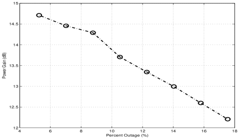
Figure 3: Two-layer cellular system power gains compared to a single layer are displayed versus percent outage for a $57$ user system.

Figure 3 shows average power gains for various outage percentages for $3$ to $10$ discarded users out of $57$ user system and this corresponds to $5\%$ to $17.5\%$ outages. Over $1000$ simulations, we observed substantial average power gains around $12-15$ dB compared to the baseline system. We also note that as we discarded more users, average power gains decreased due to decreasing degrees of freedom in the system. The previous work reported by Raman et al. shows average gains around $3$ dB when relays are deployed to predefined locations in a $19$-cell hexagonal layout [7]. The reasons for the difference between their results and in this paper is twofold. First is that in our setup, microcell base stations are always connected to macrocells through backhaul and microcells do not have to wait for macrocell transmission to decode and forward the message. This increases the degrees of freedom that the central processor has since it has more variables to further optimize the power levels. Second, there are more microcell base stations considered in our simulation setup and this brings better channel conditions between microcell base stations and users on average.

VI Conclusion

Multi-layer hierarchical cellular networks offer significant savings in total transmit power. This reduces operational expenses for the operators and at the same time, decreases global carbon dioxide emissions. Moreover, employing multiple layers in networks also helps increase coverage within the cell as well as providing higher transmission rates for low-mobility users and continuous service for vehicular users. On the other hand, increasing layers in the cellular systems creates detrimental interference within the same layer as well as in the cross layers. In this paper, we presented an analytical derivation to determine optimum power levels for two-layer networks that would minimize the total transmit power in the system and at the same time provide the same data rates. We also extended this analysis to multi-layer systems where macrocells, microcells and picocells are employed together. Through simulations we showed that significant power gains are possible when two-layers are employed in the cellular systems instead of a single-layer.

References

- [1] E. Farnworth and J. C. Castilla-Rubio, “SMART 2020: Enabling the Low Carbon Economy in the Information Age,” The Climate Group; Global e-Sustainability Initiative (GeSI), vol. 20, issue 2, pp.1-87, June 19 2008.
- [2] J. Manner, M. Luoma, J. Ott, J. Hamalainen, “Mobile Networks Unplugged,” Proc. 1st Int’l Conf. on Energy-Efficient Computing and Networking (e-Energy ’10), pp. 71-74, April 2010.
- [3] Ericsson, “Sustainable Energy Use in Mobile Communications,” Aug. 2007, White Paper.
- [4] M. Etoh, T. Ohya, Y. Nakayama, “Energy Consumption Issues on Mobile Network Systems,” Int’l Symposium on Applications and the Internet, 2008 (SAINT 2008), pp. 365-368, July-Aug, 2008.
- [5] 3GPP TR 25.942 V9.0.0, “Radio Frequency (RF) system scenarios (Release 9),” 3rd Generation Partnership Project, Technical Specification Group Radio Access Networks, Technical Report, Dec. 2009.
- [6] 3GPP TR 36.912 V. 10.0.00, “Feasibility study for Further Advancements for E-UTRA (LTE-Advanced) (Release 10),” 3rd Generation Partnership Project, Technical Specification Group Radio Access Networks, Technical Report, Mar. 2011.
- [7] C. Raman, G. J. Foschini, R. A. Valenzuela, R. D. Yates, and N. B. Mandayam, “Power savings from half-duplex relaying in downlink cellular systems,” in Proc. Allerton Conf. Commun., Control Comput. pp.748-753, Sept. 2009.
- [8] European Telecommunications Standards Institute (ETSI), “Selection Procedures for the Choice of Radio Transmission Technologies of the UMTS (UMTS 30.03 version 3.1.0),” Universal Mobile Telecommunications System, Technical Report, Nov. 1997.
- [9] P. Lancaster, Theory of Matrices. New York, NY: Academic Press, 1969.
- [10] S. A. Grandhi, R. Vijayan, D. J. Goodman, and J. Zander, “Centralized power control for cellular radio systems,” IEEE Trans. Veh. Technol., vol. 42, pp. 466-468, Nov. 1993.
- [11] J. Zander, “Performance of optimum transmitter power control in cellular radio systems,” IEEE Trans. on Veh. Technol. , vol. 41, no. 1, pp.57-62, Feb 1992.
- [12] G. J. Foschini and Z. Miljanic, “A simple distributed autonomous power control algorithm and its convergence,” IEEE Trans. Veh. Technol., vol. 42, pp. 641-646, Nov. 1993.
- [13] J. Zander, “Distributed cochannel interference control in cellular radio systems,” IEEE Trans. Veh. Technol., vol. 41, pp. 305-311, Aug. 1992.
- [14] S. A. Grandhi, R. Vijayan, and D. J. Goodman, “Distributed power control in cellular radio systems,” IEEE Trans. on Commun., vol. 42, no. 2/3/4, pp. 226-228, Feb/Mar/Apr 1994.
- [15] N. Bambos, S. C. Chen, and G. J. Pottie, “Channel access algorithms with active link protection for wireless communication networks with power control,” IEEE/ ACM Trans. Networking, vol. 8, no. 5, pp. 583-597, Oct. 2000.