Spectral dimensionality reduction for HMMs

Abstract

Hidden Markov Models (HMMs) can be accurately approximated using co-occurrence frequencies of pairs and triples of observations by using a fast spectral method Hsu et al. (2009) in contrast to the usual slow methods like EM or Gibbs sampling. We provide a new spectral method which significantly reduces the number of model parameters that need to be estimated, and generates a sample complexity that does not depend on the size of the observation vocabulary. We present an elementary proof giving bounds on the relative accuracy of probability estimates from our model. (Correlaries show our bounds can be weakened to provide either L1 bounds or KL bounds which provide easier direct comparisons to previous work.) Our theorem uses conditions that are checkable from the data, instead of putting conditions on the unobservable Markov transition matrix.

1 Introduction

For many applications such as language modeling, it is useful to estimate Hidden Markov Models (HMMs) Rabiner (1989) in which observations drawn from a large vocabulary are generated from a much smaller hidden state. Standard HMM estimation techniques such as Gibbs sampling Geman & Geman (1984) and EM Baum et al. (1970); Dempster et al. (1977) methods, although very widely used, can require some effort to apply as they are often either slow or prone to get stuck in local optima. Hsu, Kakade and Zhang, in a path breaking paper, Hsu et al. (2009) showed that HMMs can, in theory, be efficiently and accurately estimated using closed form calculations on trigrams of observations which have been projected onto a low dimensional space. Key to this approach is the use of singular value decomposition (SVD) on the matrix of covariances between adjacent observations to learn a matrix $U$ that projects observations onto a space of the same dimension as the hidden state. Perhaps surprisingly, co-occurrence statistics on unigrams, pairs, and triples of observations are sufficient to accurately estimate a model equivalent to the original HMM.

The true hidden state itself cannot, of course, be estimated (it is not observed), but one can estimate a linear transformation of the hidden state which contains sufficient information to give an optimal (in a sense to be made precise below) estimate of the probability of any sequence of observations being generated by the HMM Hsu et al. (2009). The method of Hsu et al. (2009), and the extensions to it presented in this paper do not require any EM or Gibbs sampling, but only need an SVD on bigram observation counts. Since SVD is an efficient method guaranteed to return the correct result in a known number of steps, this is a major advantage over the iterative EM method.

Hsu et al. Hsu et al. (2009) estimate a size $mv$ matrix mapping between the the dimension $v$ observation space and a reduced dimension space of size $m$ (the dimension of the hidden state space). They also need to estimate a tensor of size $vm^{2}$. We provide an alternate formulation that replaces their $vm^{2}$ tensor with one of size $m^{3}$. Since the observation vocabulary, $v$, is often much larger than the state space ($v\gg m$), this provides significant reduction in model size, and hence, as we show below, in sample complexity.

1.1 HMM set-up and notation

We now introduce the notation and model used throughout our paper.

Consider an HMM where $T$ is an $m\times m$ transition matrix on the hidden state, $O$ is a $v\times m$ emission matrix giving the probabilities of hidden state $h=j$ emitting observation $x=i$, and $\pi$ is a vector of initial state probabilities in which $\pi_{i}$ is the probability that $h_{1}=i$. Jaeger Jaeger (2000) showed that the joint probability of a sequence of observations from this HMM is given by

$$Pr(x_{1},x_{2},\ldots,x_{t})=1^{\top}A_{x_{t}}A_{x_{t-1}}\cdots A_{x_{1}}\pi,$$ (1)

where $A_{x}\equiv T\hbox{diag}(O^{\top}\delta_{x})$, $\delta_{x}$ is the unit vector of length $v$ with a single 1 in the $x$th position and $\hbox{diag}(v)$ creates a matrix with the elements of the vector $v$ on its diagonal and zeros everywhere else.

$A_{t}$ is called an ’observation operator’, an idea dating back to multiplicity automata Schutzenbeegeb (1961); Carlyle & Paz (1971); Fliess (1974), and foundational in the theory of Observable Operator Models Jaeger (2000) and Predictive State Representations Littman et al. (2002). It is effectively a third order tensor, giving the distribution vector over states at time $t+1$ as a function of the state distribution vector at the current time $t$ and the current observation $\delta_{x_{t}}$. Since $A_{t}$ depends on the hidden state, it is not observable, and hence cannot be directly estimated. But Hsu et al. (2009) showed that under certain conditions there exists a fully observable representation of the observable operator model. We now present a novel, fully reduced dimensional version of the observable representation.

1.2 The reduced dimension model

Define a random variable $y_{t}=U^{\top}\delta_{x_{t}}$, where $U$ has orthonormal columns and is a matrix mapping from observations to the reduced dimension space.

We show below that

$$Pr(x_{1},x_{2},\ldots,x_{t})=c_{\infty}^{\top}C_{y_{t}}C_{y_{t-1}}\cdots C_{y_{1}}c_{1}$$ (2)

holds where

$$c_{1} = \mu$$

$$c^{\top}_{\infty} = \mu^{\top}\Sigma^{-1}$$

$$C_{y}\equiv C(y) = K(y)\Sigma^{-1}$$

and $\mu$ = $E(y_{1})$, $\Sigma$ = $E(y_{2}y_{1}^{\top})$, and $K(a)=E(y_{3}y_{1}^{\top}y_{2}^{\top})a$ are easy to estimate using the method of moments.

The matrix $U$ can be derived in several ways; Hsu et al. (2009) show that taking it to consist of the left singular vectors of $P_{21}$ corresponding to the largest singular values gives good properties, where $P_{21}$ is a matrix such that $[P_{21}]_{ij}=Pr[x_{2}=i,x_{1}=j]$. The matrix $U$ and its properties will be discussed in more detail below.

Note that the model ($c_{1},c_{\infty},C(y)$) will be estimated using only trigrams. Once a model has been learned, the probability of any observed sequence $(x_{1},x_{2},...x_{t})$ can be computed using equation 2, or the conditional probability $Pr(x_{t}|x_{1},x_{2}...x_{t-1})$ of the next observation $x_{t}$ in a sequence can be computed by $Pr(x_{t}|x_{1:t-1})=c_{\infty}^{\top}C(y_{t})c_{t}$ with recursive updates $c_{t+1}=C(y_{t})c_{t}/(c^{\top}_{\infty}C(y_{t})c_{t})$. The key term in the model is thus $C(y)$, which can be viewed as a tensor which takes as input the current observation $x_{t}$ and produces a matrix which maps (after normalization) from the current “hidden state estimate” $c_{t}$ to the next one $c_{t+1}$. More precisely, $c_{t+1}=(U^{\top}O)\widehat{h}_{t+1}(x_{1:t})$ is a linear function of the conditional expectation of the unobservable hidden state $\widehat{h}_{t+1}(x_{1:t})$, which is the conditional probability vector over states at time $t+1$.

1.3 Comparison to Hsu et al.

Hsu et al. Hsu et al. (2009) derive a similar model which we state here for comparison.

$$Pr(x_{1},x_{2},...,x_{t})=b_{\infty}^{\top}B_{x_{t}}B_{x_{t-1}}\ldots B_{x_{1}}b_{1}$$ (3)

where

$$b_{1} = U^{\top}P_{1}$$

$$b^{\top}_{\infty} = P_{1}^{\top}(U^{\top}P_{21})^{+}$$

$$B_{x} = (U^{\top}P_{3x1})(U^{\top}P_{21})^{+}$$

and $[P_{1}]_{i}=Pr[x_{1}=i]$, $P_{21}$ as defined above, and $[P_{3x1}]_{ij}=Pr[x_{3}=i,x_{2}=x,x_{1}=j]$ are the frequencies of unigrams, bigrams, and trigrams in the observed data. Note that the subscripts on $x$ refer to their positions in trigrams of observations of the form $(x_{1},x_{2},x_{3})$.

Our major modeling change will be to replace $B_{x}$ in equation 3 with the lower dimensional tensor $C(y)$ which depends on the reduced dimension projection $y\equiv U^{\top}\delta_{x}$ instead of the unreduced $x$. The models are easily related by the following lemma:

Lemma 1.

Assume the hidden state is of dimension $m$ and the rank of $O$ is also $m$. Then:

$$Pr(x_{1},x_{2},\ldots,x_{t}) = 1^{\top}A_{x_{t}}A_{x_{t-1}}\cdots A_{x_{1}}\pi$$ (4)

$$= b_{\infty}^{\top}B_{x_{t}}B_{x_{t-1}}\cdots B_{x_{1}}b_{1}$$ (5)

$$= c_{\infty}^{\top}C_{y_{t}}C_{y_{t-1}}\cdots C_{y_{1}}c_{1}$$ (6)

Where (5) requires $U^{\top}O$ to be invertible, and (6) requires $\hbox{range}(O)\subset\hbox{range}(U)$.

Proof sketch: Paper Jaeger (2000) showed (4), paper Hsu et al. (2009) showed (5), and (6) follows from a telescoping product of the following items:

$$c_{1} = U^{\top}O\;\pi$$

$$c^{\top}_{\infty} = {\bf 1}^{\top}\;(U^{\top}O)^{-1}$$

$$C_{y}=C(y) = U^{\top}O\;A_{x}\;(U^{\top}O)^{-1}$$

where $y=U^{\top}\delta_{x}$. More details are given in the supplemental material. $\Box$

Figure 1: Two HMMs with states $h_{1}$, $h_{2}$, and $h_{3}$ which emit observations $x_{1}$, $x_{2}$, and $x_{3}$. On the left, they are further projected onto lower dimensional space with observations $y_{1}$, $y_{2}$, $y_{3}$ by $U$ from which our core statistic $C_{y}$ is computed based on $K=E(y_{3}y_{1}^{\top}y_{2}^{\top})$ which is a $(m\times m\times m)$ tensor. On the right, $x_{1}$ is hit by $(P_{21}^{\top}U)^{+}$ to make a lower dimensional $z_{1}$, $x_{2}$ is left unchanged and $x_{3}$ has its dimension reduced by $U^{\top}$. These terminal leafs are then used by Hsu et al. (2009) to estimate their $B_{x}$ via estimating $E(y_{3}z_{1}^{\top}\delta_{x_{2}}^{\top})$ which is a tensor of size $(m\times m\times v)$.

We improve Hsu et al. (2009) in three ways:

1. By reducing the size of the matrix that is estimated, we can achieve a lower sample complexity. In particular, our sample complexity does not depend on the size of the vocabulary nor on the frequency distribution of the vocabulary.

2. Since the conditions given in Hsu et al. (2009) are in terms of the transition matrix $T$, they can not be checked. We instead focus on conditions that are checkable from the data.

3. Instead of using either a L1 error or a relative entropy error, we estimate the probabilities with relative accuracy. In other words, we show that $|\widehat{p}-p|/p$ is smaller than $\epsilon$. This often is a more useful bound than just knowing $|\widehat{p}-p|$ is small. For example, it implies that computing conditional probabilities are off by less than $2\epsilon$. Both L1 and relative entropy errors can be computed from these bounds.

Our main theorem is weaker (as stated) than Hsu et al. (2009) in that we assume knowledge of $U$ rather than estimating it from a thin SVD of $P_{21}$ as they do. Since the accuracy lost when estimating $U$ is identical to that given in their paper, we will not discuss it here.

2 Theorems

The remainder of this paper presents one main theorem giving finite sample bounds for our reduced dimensional HMM estimation method. We first derive these in terms of properties of the first three moments of the reduced rank $Y$’s, where $Y$ is the random variable which takes on values of the reduced rank observation $y=U^{\top}\delta_{x}$. We then convert those bounds to be in terms of the estimates, rather than the unobservable true values, of the model.

Our general strategy of estimating $\Pr(x_{t},x_{t-1},\ldots,x_{1})$ is via the method of moments. We have $\Pr()$ written in terms of $c_{\infty}^{\top}$, $c_{1}$ and $C(y_{t})$. Since each of these three items can be written in terms of moments of the $Y$’s we can plug in these moments to generate an estimate of $\Pr()$. Thus we can define:

$$\widehat{\Pr}(x_{t},x_{t-1},\ldots,x_{1})=\widehat{c}^{\top}_{\infty}\widehat{C}(y_{t})\widehat{C}(y_{t-1})\cdots\widehat{C}(y_{1})\widehat{c}_{1}$$ (7)

where

$$\widehat{c}_{1} = \widehat{\mu}$$

$$\widehat{c}^{\top}_{\infty} = \widehat{\mu}^{\top}\widehat{\Sigma}^{-1}$$

$$\widehat{C}(y) = \widehat{K}(y)\widehat{\Sigma}^{-1}$$

where $\widehat{\mu}$, $\widehat{\Sigma}$ and $\widehat{K}()$ are the empirical estimates of the first, second and third moments of the $Y$’s, namely $\widehat{\mu}=\frac{1}{N}\sum_{i=1}^{N}Y_{1}^{(i)}$, $\widehat{\Sigma}=\frac{1}{N}\sum_{i=1}^{N}Y_{1}^{(i)}Y_{2}^{(i)\top}$, $\widehat{K}(y)=\frac{1}{N}\sum_{i=1}^{N}Y_{1}^{(i)}Y_{3}^{(i)\top}Y_{2}^{(i)\top}y$, where $Y^{(i)}$ indexes the $N$ different independent observations of our data. These moments estimate the mean vector $\mu$, the variance matrix $\Sigma$, and the skewness tensor $K()$.

Definition 1.

Define $\Lambda$ as the smallest element of $\mu$, $\Sigma^{-1}$ and $K()$. In other words,

$$\Lambda\equiv\min\{\min_{i}|\mu_{i}|,\min_{i,j}|\Sigma_{ij}^{-1}|,\min_{i,j,k}|K_{ijk}|\}$$

where we define $K_{ijk}=K(\delta_{j})_{ik}$ are the elements of the tensor $K()$. Likewise we define the empirical version as

$$\widehat{\Lambda}\equiv\min\{\min_{i}|\widehat{\mu}_{i}|,\min_{i,j}|\widehat{\Sigma}_{ij}^{-1}|,\min_{i,j,k}|\widehat{K}_{ijk}|\}$$

Definition 2.

Define $\sigma_{m}$ as the smallest singular value of $\Sigma$, and $\widehat{\sigma}_{m}$ the smallest singular value of $\widehat{\Sigma}$.

The parameters $\Lambda$ and $\sigma_{m}$ will be central to our analysis. Theorem 1 gives sample complexity bounds on relative error in estimating the probability of a sequence being generated from an HMM as a function of $\Lambda$ and $\sigma_{m}$, and the following lemmas reformulate those bounds into a more useful form in terms of their estimates. As quantified and proved below, both $\Lambda$ and $\sigma_{m}$ must be “sufficiently large”; when they approach zero one loses the ability to accurately estimate the model.

If $\sigma_{m}=0$ then $U^{\top}O$ will not be invertible, and one cannot infer the full information content of the hidden state from its associated observation, violating the condition required in Hsu et al. (2009) for (5) to hold. As $\sigma_{m}$ becomes increasingly close to zero, it becomes increasingly hard to identify the hidden state, and more observations are required. Problems with small $\sigma_{m}$ are intrinsically difficult. As has been pointed out by Hsu et al. (2009), some problems of estimating HMM’s are equivalent to the parity problem Terwijn (2002). So for such data, our algorithm need not perform well. For parity-like problems, $\sigma_{m}$ is in fact zero, or close to it; Hence we end up with a useless bound for such hard problems.

If $\Lambda$ is close to zero, then even if the absolute error is small, the relative error can be arbitrarily large, as it involves dividing by the small true value of the parameter being estimated. Fortunately, as discussed below, since $\Lambda$ depends on the somewhat arbitrary matrix $U$, one can shift $\Lambda$ away from zero by rotating and rescaling $U$.

The proof of Theorem 1 is based on the idea that if we can estimate each term in $\mu$, $\Sigma$ and $K()$ accurately on an absolute scale (which will follow from basic central limit like theorems) then we can estimate them on a relative scale if $\Lambda$ is large. Hence, our main condition is that $\Lambda$ is bounded away from zero. In fact, if we take the usual statistical limit of having the sample size $N$ go to infinity and holding everything else constant, then:

$$\left|\frac{\widehat{\Pr}(x_{1},\ldots,x_{t})}{\Pr(x_{1},\ldots,x_{t})}-1\right|\leq\frac{18mt}{\sigma_{m}^{2}\Lambda\sqrt{N}}\;\sqrt{\log(m/\delta)}$$

with probability greater than $1-\delta$ when $N$ is large enough.

The following theorem gives the finite sample bound in terms of a sample complexity:

Theorem 1.

Let $X_{t}$ be generated by an $m\geq 2$ state HMM. Suppose we are given a $U$ which has the property that $\hbox{range}(O)\subset\hbox{range}(U)$ and $|U_{ij}|\leq 1$. Suppose we use equation (7) to estimate the probability based on $N$ independent triples. Then

$$N\geq\frac{128m^{2}}{(\sqrt[2t+3]{1+\epsilon}-1)^{2}\;\Lambda^{2}\sigma_{m}^{4}}\log\left(\frac{2m}{\delta}\right)$$ (8)

implies that

$$1-\epsilon\leq\left|\frac{\widehat{\Pr}(x_{1},\ldots,x_{t})}{\Pr(x_{1},\ldots,x_{t})}\right|\leq 1+\epsilon$$

holds with probability at least $1-\delta$.

Before proceeding with the proof of this theorem, we present and prove two corollaries that correspond directly to Theorems 6 and 7 of Hsu et al. (2009).

Corollary 1.

Assume Theorem 1 holds, then with probability at least $1-\delta$,

$$\sum_{x_{1},\ldots,x_{t}}|\widehat{\Pr}(x_{t},\ldots,x_{t})-\Pr(x_{1},\ldots,x_{t})|\leq\epsilon$$

Proof of Corollary 1: We have

$$1-\epsilon\leq\left|\frac{\widehat{\Pr}(x_{1},\ldots,x_{t})}{\Pr(x_{1},\ldots,x_{t})}\right|\leq 1+\epsilon$$

$$\Rightarrow \left|\frac{\widehat{\Pr}(x_{1},\ldots,x_{t})}{\Pr(x_{1},\ldots,x_{t})}-1\right|\leq\epsilon$$

$$\Rightarrow \left|\widehat{\Pr}(x_{1},\ldots,x_{t})-\Pr(x_{1},\ldots,x_{t})\right|\leq\epsilon\Pr(x_{1},\ldots,x_{t})$$

$$\Rightarrow \sum_{x_{1},\ldots,x_{t}}\left|\widehat{\Pr}(x_{1},\ldots,x_{t})-\Pr(x_{1},\ldots,x_{t})\right|$$

$$~{}~{}~{}~{}~{}~{}~{}~{}~{}~{}~{}~{}~{}~{}~{}~{}\leq\epsilon\sum_{x_{1},\ldots,x_{t}}\Pr(x_{1},\ldots,x_{t})$$

$$\Rightarrow \sum_{x_{1},\ldots,x_{t}}\left|\widehat{\Pr}(x_{1},\ldots,x_{t})-\Pr(x_{1},\ldots,x_{t})\right|\leq\epsilon$$

$\Box$

Corollary 2.

Assume Theorem 1 holds, then we have

$$KL(\Pr(x_{t}|x_{1}, \ldots x_{t-1})||\widehat{\Pr}(x_{t}|x_{1},\ldots x_{t-1}))$$

$$=E\left(\ln\frac{\Pr(x_{t}|x_{1},\ldots x_{t-1})}{\widehat{\Pr}(x_{t}|x_{1},\ldots x_{t-1})}\right)\leq 6\epsilon$$

Proof of Corollary 2: We have

$$1-\epsilon\leq\left|\frac{\widehat{\Pr}(x_{1},\ldots,x_{t})}{\Pr(x_{1},\ldots,x_{t})}\right|\leq 1+\epsilon$$

$$\Rightarrow 1-\epsilon\leq\left|\frac{\widehat{\Pr}(x_{t}|x_{1:t-1})\widehat{\Pr}(x_{1:t-1})}{\Pr(x_{t}|x_{1:t-1})\Pr(x_{1:t-1})}\right|\leq 1+\epsilon$$

$$\Rightarrow \frac{1-\epsilon}{1+\epsilon}\leq\left|\frac{\widehat{\Pr}(x_{t}|x_{1:t-1})}{\Pr(x_{t}|x_{1:t-1})}\right|\leq\frac{1+\epsilon}{1-\epsilon}$$

and using the fact that for small enough $x$ we have $\frac{1+x}{1-x}\leq 1+3x$ and $1-3x\leq\frac{1-x}{1+x}$, plus the fact that $\epsilon_{0}\leq\frac{\epsilon}{6}$ we have

$$\Rightarrow 1-3\epsilon\leq\left|\frac{\widehat{\Pr}(x_{t}|x_{1:t-1})}{\Pr(x_{t}|x_{1:t-1})}\right|\leq 1+3\epsilon$$

$$\Rightarrow \frac{1}{1+3\epsilon}\leq\left|\frac{\Pr(x_{t}|x_{1:t-1})}{\widehat{\Pr}(x_{t}|x_{1:t-1})}\right|\leq\frac{1}{1-3\epsilon}$$

and using a similar fact from above that for small enough $x$, $\frac{1}{1-x}\leq 1+2x$, we get

$$\Rightarrow \left|\frac{\Pr(x_{t}|x_{1:t-1})}{\widehat{\Pr}(x_{t}|x_{1:t-1})}\right|\leq 1+6\epsilon$$

$$\Rightarrow \ln\left[\frac{\widehat{\Pr}(x_{t}|x_{1:t-1})}{\Pr(x_{t}|x_{1:t-1})}\right]\leq\ln(1+6\epsilon)\leq 6\epsilon$$

$$\Rightarrow \sum_{x_{1},\ldots,x_{t}}\Pr(x_{1},\ldots,x_{t})\ln\left[\frac{\widehat{\Pr}(x_{t}|x_{1:t-1})}{\Pr(x_{t}|x_{1:t-1})}\right]$$

$$~{}~{}~{}~{}~{}~{}~{}\leq 6\epsilon\sum_{x_{1},\ldots,x_{t}}\Pr(x_{1},\ldots,x_{t})$$

$$\Rightarrow E\ln\left[\frac{\widehat{\Pr}(x_{t}|x_{1:t-1})}{\Pr(x_{t}|x_{1:t-1})}\right]\leq 6\epsilon$$

$\Box$

Define $J\equiv 2m\sqrt{\frac{2\log\frac{2m}{\delta}}{N}}$ to simplify the following statements. The proof proceeds in two steps. First lemma 2 converts the sample complexity bound into a more useful bounds on $\Lambda$ and $\sigma_{m}$. Then lemma 3 uses these bounds to show the theorem.

Lemma 2.

If

$$N\geq\frac{128m^{2}}{(\sqrt[2t+3]{1+\epsilon}-1)^{2}\Lambda^{2}\sigma_{m}^{4}}\log\left(\frac{2m}{\delta}\right)$$

then

$$\Lambda \geq \frac{3J}{\sigma_{m}^{2}(\sqrt[2t+3]{1+\epsilon}-1)}$$ (9)

$$\sigma_{m} \geq 4J$$ (10)

The proof is straightforward and given in the appendix.

Lemma 3.

If equation (8) of Theorem 1 is replaced by (9) and (10) then the results of the theorem follow.

Proof of Lemma 3: Our estimator (see equation 7) can be written as

$$\widehat{\Pr}(x_{1},\ldots,x_{t})=\widehat{\mu}^{\top}\widehat{\Sigma}^{-1}\widehat{K}(y_{t})\widehat{\Sigma}^{-1}\cdots\widehat{K}(y_{1})\widehat{\Sigma}^{-1}\widehat{\mu}$$

We can rewrite this matrix product as

$$\widehat{\Pr}(x_{1},\ldots,x_{t})=$$

$$\sum_{i_{1}=1}^{m}\cdots\sum_{i_{2t+3}=1}^{m} [\widehat{\mu}]_{i_{1}}[\widehat{\Sigma}^{-1}]_{i_{1},i_{2}}[\widehat{K}(y_{t})]_{i_{2},i_{3}}[\widehat{\Sigma}^{-1}]_{i_{3},i_{4}}$$

$$\cdots[\widehat{\mu}]_{i_{2t+3}}$$

The components $[\widehat{K}(y)]_{a,b}$ can be written as a scalar sum as:

$$[\widehat{K}(y)]_{a,b}=y_{1}[\widehat{K}]_{a,b,1}+y_{2}[\widehat{K}]_{a,b,2}+\ldots+y_{m}[\widehat{K}]_{a,b,m}$$

So,

$$\widehat{\Pr}(x_{1},\ldots,x_{t})=~{}~{}~{}~{}~{}~{}~{}~{}~{}~{}~{}~{}~{}~{}~{}~{}~{}~{}~{}~{}~{}~{}~{}~{}~{}~{}~{}~{}~{}~{}~{}~{}~{}~{}~{}~{}~{}~{}~{}~{}~{}~{}~{}~{}~{}~{}~{}~{}~{}$$

$$\sum_{\begin{subarray}{c}i_{1},\ldots,i_{2t+3}\\ j_{1},\ldots,j_{t}\end{subarray}}[\widehat{\mu}]_{i_{1}}[\widehat{\Sigma}^{-1}]_{i_{1},i_{2}}[\widehat{K}]_{i_{2},i_{3},j_{1}}[y_{t}]_{j_{1}}~{}~{}~{}~{}~{}~{}~{}$$

$$\cdot[\widehat{\Sigma}^{-1}]_{i_{3},i_{4}}[\widehat{K}]_{i_{5},i_{6},j_{2}}[y_{t-1}]_{j_{2}}\;\cdots[\widehat{\mu}]_{i_{2t+3}}$$

This is just a sum of a product of scalars. Lemma 4 (stated precisely and proven in the appendix) shows that accuracy of our estimates of all elements of $\mu$, $\Sigma^{-1}$ and $K()$ are bounded by $3J/\sigma_{m}^{2}$ with probability $1-\delta$.

Each term in the product can be rewritten as

$$\widehat{\theta} = \theta\left(1+\frac{\widehat{\theta}-\theta}{\theta}\right)$$

and so our products can be thought of as, instead of a product of observed quantities, the product of the theoretical quantities times some relative error term. We can bound this relative error term for all entries, which will allow it to factor out nicely over all summands, giving us a relative error term for our overall probability.

Again thinking of $\theta$ as a generic item in $\mu$, $\Sigma$, or $K()$, then above has shown that $|\widehat{\theta}-\theta|\leq 3J/\sigma^{2}_{m}$ and so the relative error of each term is bounded as

$$1-\frac{3J}{\sigma_{m}^{2}\theta}\leq\;\frac{\widehat{\theta}}{\theta}\;\leq 1+\frac{3J}{\sigma_{m}^{2}\theta}$$

which will hold for all terms with probability $1-\delta$. Since $|\theta|\geq\Lambda$, we see that

$$1-\frac{3J}{\sigma_{m}^{2}\Lambda}\leq\;\frac{\widehat{\theta}}{\theta}\;\leq 1+\frac{3J}{\sigma_{m}^{2}\Lambda}$$

Since our $\widehat{Pr}()$ is a product of $2t+3$ such terms, we see that

$$\left(1-\frac{3J}{\sigma_{m}^{2}\Lambda}\right)^{2t+3}\leq\frac{\widehat{\Pr}()}{\Pr()}\leq\left(1+\frac{3J}{\sigma_{m}^{2}\Lambda}\right)^{2t+3}$$

So by our bound on $\Lambda$, we have

$$1-\epsilon\leq\frac{\widehat{\Pr}()}{\Pr()}\leq 1+\epsilon$$

holds with probability $1-\delta$. $\Box$

The sample complexity bound in Theorem 1 relies on knowing unobserved parameters of the problem. To avoid this, we modify Lemma 3 to make it observable. In other words, we convert the assumptions of sample complexity into a checkable condition.

Corollary 3.

Let $X_{t}$ be generated by an $m\geq 2$ state HMM. Suppose we are given a $U$ which has the property that $\hbox{range}(O)\subset\hbox{range}(U)$. Suppose we use equation (7) to estimate the probability based on $N$ independent triples. Then with probability $1-\delta$, if the following two inequalities hold

$$\widehat{\Lambda}\;\widehat{\sigma}_{m}^{2} \geq \left(12m+\frac{6m}{(\sqrt[2t+3]{1+\epsilon}-1)}\right)\sqrt{\frac{2\log\frac{2m}{\delta}}{N}}\quad$$ (11)

$$\widehat{\sigma}_{m} \geq 10m\sqrt{\frac{2\log\frac{2m}{\delta}}{N}}.$$ (12)

then

$$1-\epsilon\leq\left|\frac{\widehat{\Pr}(x_{1},\ldots,x_{t})}{\Pr(x_{1},\ldots,x_{t})}\right|\leq 1+\epsilon$$

Proof:

Two technical lemma’s are needed for this corollary: Lemma 4 and Lemma 5. They are stated and proved in the supplemental material. Lemma 4 basically says that with high probability, each element of $\mu$, $\Sigma$ and $K()$ is estimated accurately. This is then used in Lemma 5 to show that $\Lambda$ and $\sigma_{m}$ are estimated accurately.

Define the event ${\cal A}$ to be the set where all the estimates given in Lemma 4 hold. This event happens with probability $1-\delta$. On this event from Lemma 5 we know $\sigma_{m}\geq\frac{4}{5}\widehat{\sigma}_{m}$, so $\sigma_{m}^{2}\geq\frac{1}{2}\widehat{\sigma}_{m}^{2}$. Hence

$$\widehat{\Lambda}\geq\frac{6m}{\sigma_{m}^{2}(\sqrt[2t+3]{1+\epsilon}-1)}\sqrt{\frac{2\log\frac{2m}{\delta}}{N}}+\frac{6m}{\sigma_{m}^{2}}\sqrt{\frac{2\log\frac{2m}{\delta}}{N}},$$

thus on the set ${\cal A}$ if (11) and (12) hold, then we see that (9) and (10) both hold and so we can apply Theorem 1. We can now use Theorem 1 to generate our claim on the accuracy of our probability bound. Technically, this proof as given only shows that our corollary holds with probability $1-2\delta$. But since the set where Theorem 1 fails is exactly ${\cal A}^{c}$, the probability lower bound is $1-\delta$.

$\Box$

The advantage of the corollary is that the left hand sides of the two conditions are observable and the right hand sides involve known quantities. Hence one can tell if the condition is true or not–it doesn’t require knowing unobserved parameters. Note that the statement is of the form $Pr(A\Rightarrow B)\geq 1-\delta$ so interpretation must be done carefully.

3 Discussion: effect of $\Lambda$ and $\sigma_{m}$ on accuracy

As discussed above, $\sigma_{m}$ and $\Lambda$ have different effects on sample complexity. As $\sigma_{m}$ approaches zero, model estimation becomes intrinsically hard; some problems do not admit easy estimation. In contrast, role of $\Lambda$ in sample complexity is more of an artifact. As $\Lambda$ approaches zero, the relative error can be arbitrarily large, even if the estimated model is good in the sense that the probability estimates are highly accurate.

The problem with $\Lambda$ can be addressed in a couple ways. In this section, we show that estimating a likelihood ratio rather than the sequence probabilities gives improves relative accuracy bounds. An alternate approach, which we do not pursue here, relies on the observation that $\Lambda$ depends on the (underspecified) matrix $\hat{U}$, and that one can thus search for a rotation and rescaling of the matrix $\hat{U}$ that increases $\Lambda$.

3.1 Likelihood instead of probabilities

Obscure words correspond to rows of the observation matrix with very small values throughout the row. If we were interested in only estimating the probability of such a word, then these are the easy words–basically guess zero or close to it. But, since we would like to estimate the relative probability accurately, these words are the most challenging. Further, such small probabilities would make computing conditional probabilities unstable since they would then become basically “0/0.” Further, since the values are all small in $O$ and in $U$, they do not significantly improve our estimates of $\mu$, $\Sigma$ and $K()$ since they are essentially zeros. Both of these problems can be fixed by considering the problem of estimating a likelihood ratio instead of a probability. So define:

$$\lambda_{q}(x_{1},\ldots,x_{t})=\frac{Pr(x_{1},x_{2},\ldots,x_{t})}{P_{1}(x_{1})P_{1}(x_{2})\cdots P_{1}(x_{t})}$$

The $P_{1}(x)$ could be taken to be the marginal probability of observing $x$. It does not, in fact, have to be a probability–just any weighting which helps condition our matrix $\Sigma$ and our tensor $K()$. We can then use a modified version of $O$ and $U$ in all our existing lemma’s and theorems. The precise statement of these modified versions are in the appendix. What changes is that now $\Lambda$ is much larger and hence our relative accuracy will be greatly improved. This fact is shown in the empirical section.

3.2 Empirical estimates of $\Lambda$ and $\sigma_{m}$

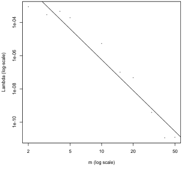
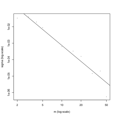
Figure 2: First graph: $\Lambda$ vs $m$, generated using vocabulary size $20,000$, Slope $\approx-6$. Second graph: $\widehat{\sigma}$ vs $m$, generated using vocabulary size of $10,000$, Slope $\approx-3.2$

Figure 2 shows estimates of $\widehat{\Lambda}$ and $\widehat{\sigma}_{m}$, using the Internet as the corpus as summarized in the Google n-gram dataset, which contains frequencies of the most frequent 1-grams to 5-grams occurring on the web. Details on how the figures were generated can be found in the supplementary material. As the size, $m$, of the reduced dimension space is increased, smaller and smaller singular values, $\sigma_{m}$, occur in the model, and the value $\Lambda$ of the smallest parameter in the model decreases. Empirically, both fall off with a power of $m$, giving straight lines on the log-log plot. This data indicates a large sample complexity, the reduction of which will be a focus of future work.

4 Prior work and conclusion

Recently, ideas have been proposed that push spectral learning of HMMs in several different directions. Boots et al. (2010) provides a kernelized spectral algorithm that allows for learning an HMM in any domain in which there exists a kernel. This allows for learning of an HMM with continuous output without the need for discretization. Boots & Gordon (2011) provides an analogous algorithm that enables online learning for Transformed Predictive State Representations, and hence the setup in Hsu et al. (2009). Finally, Siddiqi et al. (2009) directly extends Hsu et al. (2009) by relaxing the requirement that the transition matrix $T$ be of rank $m$, but instead allows rank $k\leq m$, creating a Reduced-Rank HMM (RR-HMM), and then applying the algorithm from Hsu et al. (2009) to learn the observable representation of this RR-HMM.

All of the above extensions preserve the basic structure of the tensor $B_{x}$, which updates the hidden state estimate (or more precisely, a linear transformation of it) based on the most recent observation $x$. In this paper, we replace $B_{x}$ with a tensor $C(y)$, which updates the hidden state estimate using a low dimensional projection $y$ of the observation $x$. $C(y)$ contains only $m^{3}$ terms, in contrast to the $m^{2}v$ terms contained in $B_{x}$. Reducing the number of parameters to be estimated has both computational and statistical efficiency advantages, but requires some changes to the proofs in Hsu et al. (2009). While making these changes, we also give proofs that are simpler, that only use conditions that are checkable from the data, and that bound the relative, rather than absolute error.

This paper focused on the simplest case, in which HMMs have discrete states and discrete observations and in which the observations are reduced to the same sized space as the hidden state, but our approach can be generalized in all of the ways described above.

We have presented an improved spectral method for estimating HMMs. By using a tensor $C_{y}$ that depends on the reduced rank $y$ instead of the full observed $x$ in the $B_{x}$ tensor used by Hsu et al. (2009), we reduced the number of parameters to be estimated by a factor of the ratio of the size of the vocabulary divided by the size of the hidden state. This reduction has corresponding benefits in the sample complexity. We also showed that the sample complexity depends critically upon $\sigma_{m}$, the smallest singular value of the covariance matrix $\Sigma$. As $\sigma_{m}$ becomes small, the HMM becomes increasingly hard to identify, and increasing numbers of samples are needed.

APPENDIX- SUPPLEMENTAL MATERIAL

Lemma (Restatement of Lemma 1).

Assume the hidden state is of dimension $m$ and the rank of $O$ is also $m$. Then:

$$Pr(x_{1},x_{2},\ldots,x_{t})=1^{\top}A_{x_{t}}A_{x_{t-1}}\cdots A_{x_{1}}\pi$$ (4)

$$Pr(x_{1},x_{2},\ldots,x_{t})=b_{\infty}^{\top}B_{x_{t}}B_{x_{t-1}}\cdots B_{x_{1}}b_{1}$$ (5)

$$Pr(x_{1},x_{2},\ldots,x_{t})=c_{\infty}^{\top}C_{y_{t}}C_{y_{t-1}}\cdots C_{y_{1}}c_{1}$$ (6)

Where (5) requires $U^{\top}O$ to be invertible, and (6) requires $\hbox{range}(O)\subset\hbox{range}(U)$.

Proof:

As pointed out in the main text, Jaeger (2000) showed (4), and Hsu et al. (2009) showed (5). To show (6), we will first write the characteristics $\mu$, $\Sigma$ and $K$ in terms of the theoretical matrices, $T$, $O$, $U$, and $\pi$:

$$\mu = U^{\top}O\pi$$

$$\Sigma = U^{\top}O\;T\;\hbox{diag}(\pi)\;O^{\top}U$$

$$\Sigma^{-1} = (O^{\top}U)^{-1}\;\hbox{diag}(\pi)^{-1}\;T^{-1}\;(U^{\top}O)^{-1}$$

$$K(y) = U^{\top}O\;T\;\hbox{diag}(O^{\top}Uy)\;T\;\hbox{diag}(\pi)\;O^{\top}U$$

By definition, we have

$$c_{1}\equiv\mu=U^{\top}O\;\pi$$

likewise,

$$c^{\top}_{\infty} \equiv \mu^{\top}\Sigma^{-1}$$

$$= \left(\pi^{\top}O^{\top}U\right)\left((O^{\top}U)^{-1}\;\hbox{diag}(\pi)^{-1}\right.$$

$$~{}~{}~{}~{}~{}~{}~{}~{}~{}~{}\left.\cdot\;T^{-1}\;(U^{\top}O)^{-1}\right)$$

$$= \pi^{\top}\;\hbox{diag}(\pi)^{-1}\;T^{-1}\;(U^{\top}O)^{-1}$$

$$= {\bf 1}^{\top}T^{-1}(U^{\top}O)^{-1}$$

$$= {\bf 1}^{\top}(U^{\top}O)^{-1}$$

For $C$,

$$C(y) = K(y)\;\Sigma^{-1}$$

$$= U^{\top}O\;T\;\hbox{diag}(O^{\top}Uy)\;$$

$$~{}~{}~{}~{}~{}~{}~{}~{}~{}~{}~{}\cdot\;T\;\hbox{diag}(\pi)\;O^{\top}U\;\Sigma^{-1}$$

$$= U^{\top}O\;T\;\hbox{diag}(O^{\top}Uy)(U^{\top}O)^{-1}$$

Note that $UU^{\top}$ is a projection operator and since its range is the same as that of $O$ we have $O^{\top}UU^{\top}=O^{\top}$. So, if $y=U^{\top}\delta_{x}$, then:

$$C(y) = U^{\top}O\;T\;\hbox{diag}(O^{\top}UU^{\top}\delta_{x})(U^{\top}O)^{-1}$$

$$= U^{\top}O\;T\;\hbox{diag}(O^{\top}\delta_{x})(U^{\top}O)^{-1}$$

$$= U^{\top}O\;A_{x}\;(U^{\top}O)^{-1}$$

Thus (6) follows from a telescoping product.

$\Box$

Proof of lemma 2:

The proof is simply algebraic manipulation. We have

$$N\geq\frac{128m^{2}}{(\sqrt[2t+3]{1+\epsilon}-1)^{2}\Lambda^{2}\sigma_{m}^{4}}\log\left(\frac{2m}{\delta}\right)$$

which implies that

$$\Lambda^{2} \geq \frac{128m^{2}}{(\sqrt[2t+3]{1+\epsilon}-1)^{2}N\sigma_{m}^{4}}\log\left(\frac{2m}{\delta}\right)$$

$$\geq \frac{72m^{2}}{(\sqrt[2t+3]{1+\epsilon}-1)^{2}N\sigma_{m}^{4}}\log\left(\frac{2m}{\delta}\right)$$

and taking the square root and making the relevant substitution for J we have

$$\Lambda\geq\frac{3J}{\sigma_{m}^{2}(\sqrt[2t+3]{1+\epsilon}-1)}$$

To show the bound for $\sigma_{m}$ we have that

$$N\geq\frac{128m^{2}}{(\sqrt[2t+3]{1+\epsilon}-1)^{2}\Lambda^{2}\sigma_{m}^{4}}\log\left(\frac{2m}{\delta}\right)$$

and noting that $\Lambda<1$ and $\sqrt[2t+3]{1+\epsilon}-1<1$,

$$\sigma^{4}\geq\frac{128m^{2}}{N}\log\left(\frac{2m}{\delta}\right)$$

Taking the square root of both sides and making the relevant substitution, we get

$$\sigma_{m}^{2}\geq 4J$$

and since $\sigma_{m}<1$ implies $\sigma_{m}^{2}<\sigma_{m}$ then we get the desired inequality. $\Box$

Lemma 4.

Our estimates of all elements of $\mu$, $\Sigma^{-1}$ and $K()$ are bounded by $3J/\sigma_{m}^{2}$ with probability $1-\delta$, where $J\equiv 2m\sqrt{\frac{2\log\frac{2m}{\delta}}{N}}$.

Proof:

We first derive absolute bounds for each entry of $\mu$, $\Sigma$ and $K()$. To handle all three of them at the same time, we will generically call any one of these three “$\theta$” and its estimate $\widehat{\theta}$. Suppose that $\widehat{\theta}$ has $g$ entries that are taking the mean with $N$ observations all of which are bounded between $-1$ and $1$. Then, for each entry we have from Hoeffding (1963) that

$$Pr(|\widehat{\theta}_{i}-\theta_{i}|>\epsilon)\leq 2e^{\frac{-N\epsilon^{2}}{2}}$$

and so

$$Pr(\exists~{}i~{}\mathrm{s.t.}~{}|\widehat{\theta}_{i}-\theta_{i}|>\epsilon)\leq 2ge^{\frac{-N\epsilon^{2}}{2}}$$

and setting $2ge^{\frac{-N\epsilon^{2}}{2}}=\delta$ we solve that $\epsilon=\sqrt{\frac{2\log\frac{2g}{\delta}}{N}}$ so with probability $1-\delta$ we have that

$$\forall i\quad|\widehat{\theta}_{i}-\theta_{i}|\leq\sqrt{\frac{2\log\frac{2g}{\delta}}{N}}.$$

Note that for $\mu$, $\Sigma$ and $K()$ we have a vector, a matrix and a tensor that are estimated as $E(Y_{1})$, $E(Y_{1}Y_{2}^{\top})$ and $E(Y_{3}Y_{1}^{\top}Y_{2}^{\top})$ respectively with $m$, $m^{2}$ and $m^{3}$ entries respectively, we see that the total number of entries in all three of them is less than $m^{4}$. (Except in the trivial case where $m=1$. But this corresponds to the data being IID and so doesn’t count as a HMM.) So all three of the following hold simultaneously with probability $1-\delta$:

$$\forall i\quad|\widehat{\mu}_{i}-\mu_{i}| \leq \sqrt{\frac{8\log\frac{2m}{\delta}}{N}}$$

$$\forall i,j\quad|\widehat{\Sigma}_{ij}-\Sigma_{ij}| \leq \sqrt{\frac{8\log\frac{2m}{\delta}}{N}}$$ (13)

$$\forall i,j,j\quad|[\widehat{K}]_{ijk}-[K]_{ijk}| \leq \sqrt{\frac{8\log\frac{2m}{\delta}}{N}}$$

Lastly we need to bound $\Sigma^{-1}$. We will start by bounding the norm of $\widehat{\Sigma}-\Sigma$. By (13) we see $||\widehat{\Sigma}-\Sigma||_{\max}\leq\sqrt{\frac{8\log\frac{2m}{\delta}}{N}}$, by the relationship $||M||_{2}\leq m||M||_{\max}$ for $m\times m$ square matrices, we get the desired result.

From this bound on $||\widehat{\Sigma}-\Sigma||_{2}$ and lemma 20 of Hsu et al. (2009) we have that

$$|\widehat{\sigma}_{m}-\sigma_{m}|\leq J$$ (14)

where $\sigma_{m}$ is the smallest singular value for $\Sigma$. By their Lemma 23 we then have that

$$||\widehat{\Sigma}^{-1}-\Sigma^{-1}||_{2}\leq\frac{1+\sqrt{5}}{2}\left(\frac{1}{\widehat{\sigma}_{m}-J}\right)^{2}J$$

By assumption $\sigma_{m}>4J$, we see $\sigma_{m}-J>3\sigma_{m}/4$. Thus from the algebra that $\frac{1+\sqrt{5}}{2}(\frac{4}{3})^{2}\leq 3$, we see

$$||\widehat{\Sigma}^{-1}-\Sigma^{-1}||_{2}\leq 3J/\sigma_{m}^{2}.$$

From $||\widehat{\Sigma}^{-1}-\Sigma^{-1}||_{\max}\leq||\widehat{\Sigma}^{-1}-\Sigma^{-1}||_{2}$ we get our element-wise norm on the errors. Since $\sigma_{m}\leq 1$, we see that

$$3J/\sigma_{m}^{2}\geq 3J=3m\sqrt{\frac{8\log\frac{2m}{\delta}}{N}}\geq\sqrt{\frac{8\log\frac{2m}{\delta}}{N}}$$

$\Box$

Lemma 5.

The estimates of $\Lambda$ and $\sigma_{m}$ have the following accuracy:

$$|\widehat{\Lambda}-\Lambda| \leq \frac{6m}{\sigma_{m}^{2}}\sqrt{\frac{2\log\frac{2m}{\delta}}{N}}$$

$$|\widehat{\sigma}_{m}-\sigma_{m}| \leq 2m\sqrt{\frac{2\log\frac{2m}{\delta}}{N}}.$$

with probability greater than $1-\delta$.

Proof: $\widehat{\Lambda}$ is the empirical minimum of all the

$$\widehat{\Lambda}\equiv\min\{\min_{i}|\widehat{\mu}_{i}|,\min_{i,j}|\widehat{\Sigma}_{ij}^{-1}|,\min_{i,j,k}|\widehat{K}_{i,j,k}|\}$$

From lemma 4 we have bounded the accuracy of the estimate of each element of $\mu$, $\Sigma$ and $K()$, the minimum of these will be estimated within the same accuracy. This established (5).

The second inequality (5) was also established in the proof of the theorem in equation (14).

$\Box$

5 Likelihood ratio version of theorem 1

In 3.1 we considered the likelihood ratio as a way of getting a better estimator. There we used a weighting vector $p_{i}$ which normalized our probability. In other words,

$$\frac{Pr(x_{1},x_{2},\ldots,x_{t})}{p_{x_{1}}p_{x_{2}}\cdots p_{x_{t}}}$$

It will be a bit more mathematically convenient if we instead use $q_{i}=1/\sqrt{p_{i}}$ instead. So, define:

$$Q(x_{1:t})=Q(x_{1},x_{2},\ldots,x_{t})=q(x_{1})q(x_{2})\cdots q(x_{t})$$

Then our “likelihood ratio” is

$$\lambda(x_{1},x_{2},\ldots,x_{t})=Pr(x_{1},x_{2},\ldots,x_{t})Q(x_{1},x_{2},\ldots,x_{t})^{2}$$

We will think of these $q_{i}$’s as a vector and define

$$O^{*}\equiv\hbox{diag}(q)O$$

and

$$A^{*}_{x}\equiv T\hbox{diag}(O^{*T}\hbox{diag}(q)\delta_{x})$$

We will then be able to show a similar product rule as (1):

$$Pr(x_{1:t})Q^{2}(x_{1:t})=1^{\top}A^{*}_{x_{t}}A^{*}_{x_{t-1}}\cdots A^{*}_{x_{1}}\pi.$$

The version of this product rule we will estimate is also similar. We will define $U^{*}=\hbox{diag}(q)U$ and $y^{*}_{t}=U^{*\top}\hbox{diag}(q)\delta_{x_{t}}=U^{\top}\hbox{diag}(q)^{2}\delta_{x_{t}}$. Our statistics are then:

$$\mu^{*} \equiv E(y^{*}_{1})$$

$$\Sigma^{*} \equiv E(y^{*}_{2}y^{*\top}_{1})$$

$$K^{*}(a) \equiv E(y^{*}_{3}y^{*\top}_{1}y^{*\top}_{2})a$$

Defining our characteristics as before:

$$c^{*}_{1} \equiv \mu^{*}$$

$$c^{*\top}_{\infty} \equiv \mu^{*\top}\Sigma^{*-1}$$

$$C^{*}(y^{*}) = K^{*}(y^{*})\;\Sigma^{*-1}$$

These can also be used to estimate $\lambda$ as the following lemma shows:

Lemma 6.

Assume the hidden state is of dimension $m$ and the rank of $O$ is also $m$. Then:

$$\lambda(x_{1},\ldots,x_{t}) \equiv Pr(x_{1:t})Q^{2}(x_{1:t})$$ (15)

$$= 1^{\top}A^{*}_{x_{t}}A^{*}_{x_{t-1}}\cdots A^{*}_{x_{1}}\pi$$

$$= c^{*\top}_{\infty}C^{*}(y^{*}_{t})\cdots C^{*}(y^{*}_{1})c^{*}_{1}$$

Where the last equation requires
$\hbox{range}(O)\subset\hbox{range}(U\hbox{diag}(q))$.

Proof:

$$A^{*}_{x} \equiv T\;\hbox{diag}(O^{*\top}\hbox{diag}(q)\delta_{x})$$

$$= T\;\hbox{diag}((\hbox{diag}(q)O)^{\top}\hbox{diag}(q)\delta_{x})$$

$$= T\;\hbox{diag}(O^{\top}\hbox{diag}(q)^{2}\delta_{x})$$

$$= T\;\hbox{diag}(O^{\top}\hbox{diag}(q)^{2}\hbox{diag}(\delta_{x}){\bf 1})$$

$$= T\;\hbox{diag}(O^{\top}\hbox{diag}(\delta_{x})^{2}\hbox{diag}(q)^{2}{\bf 1})$$

$$= T\;\hbox{diag}(O^{\top}\hbox{diag}(\delta_{x})(q^{2}_{x}))$$

$$= T\;\hbox{diag}(O^{\top}\delta_{x})\;q^{2}_{x}$$

$$= A_{x}\;q^{2}_{x}$$

where we have used $a^{\top}\hbox{diag}(\delta_{x})b=(a^{\top}\delta_{x})\;(b^{\top}\delta_{x})$.

Our “starred” versions can be written in terms of the basic items $T$, $O$, $U$, $\pi$ and $q$:

$$\mu^{*} = U^{\top}\hbox{diag}(q)^{2}O\pi$$

$$\Sigma^{*} = U^{\top}\hbox{diag}(q)^{2}O\;T\;\hbox{diag}(\pi)\;O^{\top}\hbox{diag}(q)^{2}U$$

$$\Sigma^{*-1} = (O^{\top}\hbox{diag}(q)^{2}U)^{-1}\;\hbox{diag}(\pi)^{-1}\;$$

$$~{}~{}~{}~{}~{}~{}~{}~{}\cdot\;T^{-1}\;(U^{\top}\hbox{diag}(q)^{2}O)^{-1}$$

$$K^{*}(x) = U^{\top}\hbox{diag}(q)^{2}O\;T\;\hbox{diag}(O^{\top}\hbox{diag}(q)^{2}Ux)\;$$

$$~{}~{}~{}~{}~{}~{}~{}~{}\cdot\;T\;\hbox{diag}(\pi)\;O^{\top}\hbox{diag}(q)^{2}U$$

So, we have

$$c^{*}_{1}\equiv\mu^{*}=U^{\top}\hbox{diag}(q)^{2}O\;\pi$$

likewise,

$$c^{*\top}_{\infty} \equiv \mu^{*\top}\Sigma^{*-1}$$

$$= \left(\pi^{\top}O^{\top}\hbox{diag}(q)^{2}U\right)$$

$$~{}~{}~{}~{}~{}~{}~{}~{}~{}~{}~{}~{}\cdot\;\left((O^{\top}\hbox{diag}(q)^{2}U)^{-1}\;\hbox{diag}(\pi)^{-1}\;\right.$$

$$~{}~{}~{}~{}~{}~{}~{}~{}~{}~{}~{}~{}~{}~{}~{}~{}~{}~{}~{}~{}~{}~{}\cdot\;\left.T^{-1}\;(U^{\top}\hbox{diag}(q)^{2}O)^{-1}\right)$$

$$= \pi^{\top}\;\hbox{diag}(\pi)^{-1}\;T^{-1}\;(U^{\top}\hbox{diag}(q)^{2}O)^{-1}$$

$$= {\bf 1}^{\top}T^{-1}(U^{\top}\hbox{diag}(q)^{2}O)^{-1}$$

$$= {\bf 1}^{\top}(U^{\top}\hbox{diag}(q)^{2}O)^{-1}$$

For $C^{*}$ we

$$C^{*}(y) = K^{*}(y)\;\Sigma^{*-1}$$

$$= U^{\top}\hbox{diag}(q)^{2}O\;T\;\hbox{diag}(O^{\top}\hbox{diag}(q)^{2}Uy)\;$$

$$~{}~{}~{}~{}~{}\cdot\;T\;\hbox{diag}(\pi)\;O^{\top}\hbox{diag}(q)^{2}U\;\Sigma^{*-1}$$

$$= U^{\top}\hbox{diag}(q)^{2}O\;T\;\hbox{diag}(O^{\top}\hbox{diag}(q)^{2}Uy)$$

$$~{}~{}~{}~{}~{}~{}~{}~{}~{}\cdot\;(U^{\top}\hbox{diag}(q)^{2}O)^{-1}$$

Note that $U^{*}U^{*\top}$ is an $n\times n$ projection operator. Since its range is the same as that of $O^{*}$ we have $O^{*\top}U^{*}U^{*\top}=O^{*\top}$. So, if $y^{*}=U^{*\top}\hbox{diag}(q)\delta_{x}$, then:

$$C^{*}({y^{*}}) = U^{\top}\hbox{diag}(q)^{2}O\;T\;$$

$$\cdot\;\hbox{diag}(O^{*\top}U^{*}U^{*\top}\hbox{diag}(q)\delta_{x})$$

$$~{}~{}~{}~{}~{}~{}~{}~{}~{}~{}~{}~{}~{}\cdot\;(U^{\top}\hbox{diag}(q)^{2}O)^{-1}$$

$$= U^{\top}\hbox{diag}(q)^{2}O\;T\;\hbox{diag}(O^{\top}\hbox{diag}(q)^{2}\delta_{x})$$

$$~{}~{}~{}~{}~{}\cdot\;(U^{\top}\hbox{diag}(q)^{2}O)^{-1}$$

$$= (U^{\top}\hbox{diag}(q)^{2}O)\;A^{*}_{x}\;(U^{\top}\hbox{diag}(q)^{2}O)^{-1}$$

Hence equation (15) follows by a telescoping product.

$\Box$

Theorem 2.

Let $X_{t}$ be generated by an $m\geq 2$ state HMM. Suppose we are given a $U$ which has the property that $\hbox{range}(O)\subset\hbox{range}(U)$ and $|U_{ij}|\leq 1$. Suppose we use equation (15) to estimate $\lambda(x_{1},x_{2},\ldots,x_{t})$ based on $N$ independent triples and for appropriate choice of $U^{*}$. Then the following two inequalities

$$\Lambda^{*} \geq \frac{6m}{\sigma_{m}^{*2}(\sqrt[2T+3]{1+\epsilon}-1)}\sqrt{\frac{2\log\frac{2m}{\delta}}{N}}$$ (16)

$$\sigma_{m}^{*} \geq 8m\sqrt{\frac{2\log\frac{2m}{\delta}}{N}}.$$ (17)

(where $\sigma_{m}^{*}$ is the smallest eigenvalue of $\Sigma^{*}$) imply

$$1-\epsilon\leq\left|\frac{\widehat{\lambda}(x_{1},\ldots,x_{t})}{\lambda(x_{1},\ldots,x_{t})}\right|\leq 1+\epsilon$$

or equivalently

$$1-\epsilon\leq\left|\frac{\widehat{\Pr}(x_{1},\ldots,x_{t})}{\Pr(x_{1},\ldots,x_{t})}\right|\leq 1+\epsilon$$

holds with probability at least $1-\delta$.

Proof:

The proof of this goes is identical to that given for theorem 1. The only worry is that we have defined $y^{*}$’s differently. But since we only required $|y|\leq 1$, and we have constructed $|y^{*}|\leq 1$, the Hoeffding inequality with elements of $U$ still hold for $U^{*}$.

$\Box$

Details of generating the graphs

In lemma 6 and theorem 2 we see that we can increase our chances of obtaining a large enough $\Lambda$ by multiplying each row of $U$ by some function of that row. As long as we ensure that the elements of our new $U^{*}$ are less than one, then we can make a claim on the accuracy of the relative "likelihood", and hence the relative probability, generated by our sample.

Our figures utilize this gain in the size of $\Lambda$. For our corpus we use the Internet as captured by the Google n-gram dataset. We first create a dictionary of the $v-1$ most popular tokens, as well as an "out of vocabulary" token, for a final dictionary of size $v$. We take $U$ to be the $U$ matrix generated by the ’thin’ SVD of the $P_{21}$ matrix generated using this vocabulary and Google 2-grams.

From this $U$ we consider the first $m$ columns. As per above, we can increase our chances of obtaining a large enough $\Lambda$ by maximizing the size of the entries in this new $v\times m$ dimensional $U$ matrix, hence we multiply each row by $1/\max_{j}(|U_{i,j}|)$, ensuring that at least one of the elements in our matrix is exactly $1$ or $-1$. Now, using this new matrix $U^{*}$ we use the frequencies from Google 1-grams, 2-grams, and 3-grams to compute $\mu^{*}$, $\Sigma^{*}$, and $K^{*}$ respectively, where each of the $v$ vocabulary words (including one out-of-vocabulary token) correspond to a row of $U^{*}$. From this, we take $\Sigma^{*-1}$ and compute the minimum element across $\mu^{*}$, $\Sigma^{*-1}$ and $K^{*}$.

We obtain $\sigma^{*}_{m}$ in a similar way, first computing $\Sigma^{*}$ from the appropriate $v\times m$ dimensional $U^{*}$ matrix, then taking the SVD, recording the smallest singular value.

References

Baum et al. (1970)
Baum, L.E., Petrie, T., Soules, G., and Weiss, N.
A maximization technique occurring in the statistical analysis of
probabilistic functions of markov chains.
The annals of mathematical statistics, 41(1):164–171, 1970.
Boots & Gordon (2011)
Boots, B. and Gordon, G.J.
An online spectral learning algorithm for partially observable
nonlinear dynamical systems.
AAAI, 2011.
Boots et al. (2010)
Boots, B., Siddiqi, S.M., Gordon, G., and Smola, A.
Hilbert space embeddings of hidden markov models.
Proc. 27th Intl. Conf. on Machine Learning (ICML), 2010.
Carlyle & Paz (1971)
Carlyle, J.W. and Paz, A.
Realizations by stochastic finite automata.
Journal of Computer and System Sciences, 5(1):26–40, 1971.
Dempster et al. (1977)
Dempster, A.P., Laird, N.M., and Rubin, D.B.
Maximum likelihood from incomplete data via the em algorithm.
Journal of the Royal Statistical Society. Series B
(Methodological), 39(1):1–38, 1977.
Fliess (1974)
Fliess, M.
Matrices de hankel.
J. Math. Pures Appl, 53(197-222):423,
1974.
Geman & Geman (1984)
Geman, Stuart and Geman, Donald.
Stochastic relaxation, gibbs distributions, and the bayesian
restoration of images.
Pattern Analysis and Machine Intelligence, IEEE Transactions
on, PAMI-6(6):721 –741, nov. 1984.
ISSN 0162-8828.
doi: 10.1109/TPAMI.1984.4767596.
Hoeffding (1963)
Hoeffding, Wassily.
Probability inequalities for sums of bounded random variables.
Journal of the American Statistical Association, 58(301):pp. 13–30, 1963.
ISSN 01621459.
URL http://www.jstor.org/stable/2282952.
Hsu et al. (2009)
Hsu, Daniel, Kakade, Sham M., and Zhang, Tong.
A spectral algorithm for learning hidden markov models.
COLT, 2009.
Jaeger (2000)
Jaeger, Herbert.
Observable operator models for discrete stochastic time series.
Neural Computation, 12(6), 2000.
Littman et al. (2002)
Littman, M.L., Sutton, R.S., and Singh, S.
Predictive representations of state.
Advances in neural information processing systems, 2:1555–1562, 2002.
Rabiner (1989)
Rabiner, L.R.
A tutorial on hidden markov models and selected applications in
speech recognition.
Proceedings of the IEEE, 77(2):257–286,
1989.
Schutzenbeegeb (1961)
Schutzenbeegeb, MP.
On the definition of a family of automata.
Information and control, 4(2-3), 1961.
Siddiqi et al. (2009)
Siddiqi, S.M., Boots, B., and Gordon, G.J.
Reduced-rank hidden markov models.
Arxiv preprint arXiv:0910.0902, 2009.
Terwijn (2002)
Terwijn, S.
On the learnability of hidden markov models.
Grammatical Inference: Algorithms and Applications, pp. 344–348, 2002.