Accuracy and Stability of Filters for Dissipative PDEs

Abstract

Data assimilation methodologies are designed to incorporate noisy observations of a physical system into an underlying model in order to infer the properties of the state of the system. Filters refer to a class of data assimilation algorithms designed to update the estimation of the state in an on-line fashion, as data is acquired sequentially. For linear problems subject to Gaussian noise, filtering can be performed exactly using the Kalman filter. For nonlinear systems filtering can be approximated in a systematic way by particle filters. However in high dimensions these particle filtering methods can break down. Hence, for the large nonlinear systems arising in applications such as oceanography and weather forecasting, various ad hoc filters are used, mostly based on making Gaussian approximations. The purpose of this work is to study the accuracy and stability properties of these ad hoc filters. We work in the context of the 2D incompressible Navier-Stokes equation, although the ideas readily generalize to a range of dissipative partial differential equations (PDEs). By working in this infinite dimensional setting we provide an analysis which is useful for the understanding of high dimensional filtering, and is robust to mesh-refinement. We describe theoretical results showing that, in the small observational noise limit, the filters can be tuned to perform accurately in tracking the signal itself (filter accuracy), provided the system is observed in a sufficiently large low dimensional space; roughly speaking this space should be large enough to contain the unstable modes of the linearized dynamics. The tuning corresponds to what is known as variance inflation in the applied literature. Numerical results are given which illustrate the theory. The positive results herein concerning filter stability complement recent numerical studies which demonstrate that the ad hoc filters can perform poorly in reproducing statistical variation about the true signal.

1 Introduction

Assimilating large data sets into mathematical models of time-evolving systems presents a major challenge in a wide range of applications. Since the data and the model are often uncertain, a natural overarching framework for the formulation of such problems is that of Bayesian statistics. However, for high dimensional models, investigation of the Bayesian posterior distribution of model state given data is not computationally feasible in on-line situations. For this reason various ad hoc filters are used. The purpose of this paper is to provide an analysis of such filters.

The paradigmatic example of data assimilation is weather forecasting: computational models to predict the state of the atmosphere currently involving on the order of ${\mathcal{O}}(10^{8})$ unknowns but these models must be run with an initial condition which is only known incompletely. This is compensated for by a large number, currently on the order of ${\mathcal{O}}(10^{6})$, partial observations of the atmosphere at subsequent times. Filters are widely used to make forecasts which combine the mathematical model of the atmosphere and the data to make predictions. Indeed the particular method of data assimilation which we study here includes, as a special case, the algorithm commonly known as 3DVAR. This method originated in weather forecasting. It was first proposed at the UK Met Office in 1986 [1], and was developed by the US National Oceanic and Atmospheric Administration (NOAA) soon thereafter; see [2]. More details of the implementation of 3DVAR by the UK Met Office can be found in [3], and by the European Centre for Medium-Range Weather Forecasts (ECMWF) in [4]. The 3DVAR algorithm is prototypical of the many more sophisticated filters which are now widely used in practice and it is thus natural to study it. The reader should be aware, however, that the development of new filters is a very active area and that the analysis here constitutes an initial step towards the analyses required for these more recently developed algorithms. For insight into some of these more sophisticated filters see [5, 6, 7, 8, 9] and the references therein.

Filtering can be performed exactly for linear systems subject to Gaussian noise: the Kalman filter [10]. For nonlinear or non-Gaussian scenarios the particle filter [11] may be used and provably approximates the desired probability distribution as the number of particles is increased [12]. However in practice this method performs poorly in high dimensional systems [13]. Whilst there is considerable research activity aimed at overcoming this degeneration [14, 15], the methodology cannot yet be viewed as a provably accurate tool within the context of the high dimensional problems arising in geophysical data assimilation. In order to circumvent problems associated with the representation of high dimensional probability distributions some form of ad hoc Gaussian approximation is typically used to create practical filters, and the 3DVAR method which we analyze here is perhaps the simplest example of this. This ad hoc filters may also be viewed in the framework of nonlinear control theory. Proving filter stability and accuracy has a long history in this field and the paper [16] is closely related to the work we develop here. However we work in an infinite dimensional setting, in order to directly confront the high dimensionality of many current real-world filtering applications, and this brings new issues to the problem of establishing filter stability and accuracy; overcoming these problems provides the focus of this paper.

In the paper [17] a wide range of Gaussian approximate filters, including 3DVAR, are evaluated by comparing the distributions they produce with a highly accurate (and impractical in realistic online scenarios) MCMC simulation of the desired distributions. The conclusion of that work is that the Gaussian approximate filters perform well in tracking the mean of the desired distribution, but poorly in terms of statistical variability about the mean. In this paper we provide a theoretical analysis of the ability of the filters to estimate the mean state accurately. Although filtering is widely used in practice, much of the analysis of it, in the context of fluid mechanics, works with finite-dimensional dynamical models. Our aim is to work directly with a PDE model relevant in fluid mechanics, the Navier-Stokes equation, and thereby confront the high-dimensional nature of the problem head-on. Study of the stability of filters for data assimilation has been a developing research area over the last few years and the paper [18] contains a finite dimensional theoretical result, numerical experiments in a variety of finite and (discretized) infinite dimensional systems not covered by the theory, and references to relevant applied literature. The paper [19] gives a review of many important aspects relating to assimilating the evolving unstable directions of the underlying dynamical system. Our analysis will build in a concrete fashion on the approach in [20] and [21] which were amongst the first to study data assimilation directly through PDE analysis, using ideas from the theory of determining modes in infinite dimensional dynamical systems. However, in contrast to those papers, we will allow for noisy observations in our analysis. Nonetheless the estimates in [21] form an important component of our analysis. Furthermore the large time asymptotic results in [21] constitute a limiting case of our theory, where there is no observational noise.

The presentation will be organized as follows: in Section 2 we introduce the Navier-Stokes equation as the forward model of interest and formulate the inverse problem of estimating the velocity field given partial noisy observations. This leads to a family of filters for the velocity field which have the form of a non-autonomous dynamical system which blends the forward model with the data in a judicious fashion; Theorem 2.3 describes this dynamical system via the solution of a sequence of inverse problems. In Section 3 we introduce notions of stability and prove the Main Theorems 3.3 and 3.7 concerning filter stability and accuracy for sufficiently small observational noise. In Section 4 we present numerical results which corroborate the analysis; and finally, in Section 5 we present conclusions.

2 Combining Model and Data

In subsection 2.1 we describe the forward model that we employ throughout the remainder of the paper: the Navier Stokes equation on a two dimensional torus. Then, in subsection 2.2, we describe the observational data model that we employ; using this we apply Tikhonov-Phillips regularization to derive the filter which we use to combine model and data. Subsection 2.3 contains a specific example of this filter, used later in the paper for our numerical illustrations. This example constitutes a particular instance of the 3DVAR method.

2.1 Forward Model: Navier-Stokes equation

In this section we establish a notation for, and describe the properties of, the Navier-Stokes equation. This is the forward model which underlies the inverse problem which we study in this paper. We consider the 2D Navier-Stokes equation on the torus $\mathbb{T}^{2}:=[0,L)\times[0,L)$ with periodic boundary conditions:

$$\begin{array}[]{cccc}\partial_{t}u-\nu\Delta u+u\cdot\nabla u+\nabla p&=&f&{\rm for~{}all~{}}(x,t)\in\mathbb{T}^{2}\times(0,\infty),\\ \nabla\cdot u&=&0&{\rm for~{}all~{}}(x,t)\in\mathbb{T}^{2}\times(0,\infty),\\ u(x,0)&=&u_{0}(x)&{\rm for~{}all~{}}x\in\mathbb{T}^{2}.\end{array}$$

Here $u\colon\mathbb{T}^{2}\times(0,\infty)\to\mathbb{R}^{2}$ is a time-dependent vector field representing the velocity, $p\colon\mathbb{T}^{2}\times(0,\infty)\to\mathbb{R}$ is a time-dependent scalar field representing the pressure, $f\colon\mathbb{T}^{2}\to\mathbb{R}^{2}$ is a vector field representing the forcing (which we assume to be time-independent for simplicity), and $\nu$ is the viscosity. In numerical simulations (see section 4), we typically represent the solution via the vorticity $w$ and stream function $\zeta$; these are related through $u=\nabla^{\perp}\zeta$ and $w=\nabla^{\perp}\cdot u$, where $\nabla^{\perp}=(\partial_{2},-\partial_{1})^{\mathrm{T}}$. We define

$${\mathcal{H}}:=\left\{{\rm{trigonometric\,polynomials\,}}u:\mathbb{T}^{2}\to{\mathbb{R}}^{2}\,\Bigl{|}\,\nabla\cdot u=0,\,\int_{\mathbb{T}^{2}}u(x)\,\mathrm{d}x=0\right\}$$

and $H$ as the closure of ${\mathcal{H}}$ with respect to the $(L^{2}(\mathbb{T}^{2}))^{2}$ norm. We define $P:(L^{2}(\mathbb{T}^{2}))^{2}\to H$ to be the Leray-Helmholtz orthogonal projector.

Given $k=(k_{1},k_{2})^{\mathrm{T}}$, define $k^{\perp}:=(k_{2},-k_{1})^{\mathrm{T}}$. Then an orthonormal basis for $H$ is given by $\psi_{k}\colon\mathbb{R}^{2}\to\mathbb{R}^{2}$, where

$$\psi_{k}(x):=\frac{k^{\perp}}{|k|}\exp\Bigl{(}\frac{2\pi ik\cdot x}{L}\Bigr{)}\quad{\rm for}\quad k\in\mathbb{Z}^{2}\setminus\{0\}.$$ (2)

Thus for $u\in H$ we may write

$$u=\sum_{k\in\mathbb{Z}^{2}\setminus\{0\}}u_{k}(t)\psi_{k}(x)$$

where, since $u$ is a real-valued function, we have the reality constraint $u_{-k}=-\overline{u_{k}}.$ We then define the projection operators $P_{\lambda}:H\to H$ and $Q_{\lambda}:H\to H$ by

$$P_{\lambda}u=\sum_{|2\pi k|^{2}<\lambda L^{2}}u_{k}(t)\psi_{k}(x),\quad Q_{\lambda}=I-P_{\lambda}.$$

We let $W_{\lambda}=P_{\lambda}H$ and $W_{\lambda}^{c}=Q_{\lambda}H.$

Using the Fourier decomposition of $u$, we define the fractional Sobolev spaces

$$H^{s}:=\left\{u\in H:\sum_{k\in\mathbb{Z}^{2}\setminus\{0\}}(4\pi^{2}|k|^{2})^{s}|u_{k}|^{2}<\infty\right\}$$ (3)

with the norm $\|u\|_{s}:=\bigl{(}\sum_{k}(4\pi^{2}|k|^{2})^{s}|u_{k}|^{2}\bigr{)}^{1/2}$, where $s\in\mathbb{R}$. We use the abbreviated notation $\|u\|$ for the norm on $H^{1}$, and $|\cdot|$ for the norm on $H=H^{0}$.

Applying the projection $P$ to the Navier-Stokes equation we may write it as an ODE (ordinary differential equation) in $H$; see [22, 23, 24] for details. This ODE takes the form

$$\frac{\mathrm{d}u}{\mathrm{d}t}+\nu Au+\mathcal{B}(u,u)=f,\quad u(0)=u_{0}.$$ (4)

Here, $A=-P\Delta$ is the Stokes operator, the term $\mathcal{B}(u,u)=P(u\cdot\nabla u)$ is the bilinear form found by projecting the nonlinear term $u\cdot\nabla u$ onto $H$ and finally, with abuse of notation, $f$ is the original forcing, projected into $H$. We note that $A$ is diagonalized in the basis comprised of the $\{\psi_{k}\}_{k\in{\mathbb{Z}}^{2}\backslash\{0\}}$, on $H$, and the smallest eigenvalue of $A$ is $\lambda_{1}=4\pi^{2}/L^{2}.$ The following proposition is a classical result which implies the existence of a dissipative semigroup for the ODE Eq. ( 4 ). See Theorems 9.5 and 12.5 in [24] for a concise overview and [23, 25] for further details.

Proposition 2.1.

Assume that $u_{0}\in H^{1}$ and $f\in H$. Then Eq. ( 4 ) has a unique strong solution on $t\in[0,T]$ for any $T>0:$

$$u\in L^{\infty}\bigl{(}(0,T);H^{1}\bigr{)}\cap L^{2}\bigl{(}(0,T);D(A)\bigr{)},\quad\frac{du}{dt}\in L^{2}\bigl{(}(0,T);H\bigr{)}.$$

Furthermore the equation has a global attractor $\mathcal{A}$ and there is $K>0$ such that, if $u_{0}\in\mathcal{A}$, then $\sup_{t\geq 0}\|u(t)\|^{2}\leq K.$

We let $\{\Psi(\cdot,t):H^{1}\to H^{1}\}_{t\geq 0}$ denote the semigroup of solution operators for the equation Eq. ( 4 ) through $t$ time units. We note that by working with weak solutions, $\Psi(\cdot,t)$ can be extended to act on larger spaces $H^{s}$, with $s\in[0,1)$, under the same assumption on $f$; see Theorem 9.4 in [24]. We will, on occasion, use this extension of $\Psi(\cdot,t)$ to act on larger spaces.

The key properties of the Navier-Stokes equation that drive our analysis of the filters are summarized in the following proposition, taken from the paper [21]. To this end, define $\Psi(\cdot)=\Psi(\cdot,h)$ for some fixed $h>0.$ Note that the statement here is closely related to the squeezing property [24] of the Navier-Stokes equation, a property employed in a wide range of applied contexts. Furthermore, many other dissipative PDEs are known to satisfy similar properties.

Proposition 2.2.

Let $u\in\mathcal{A}$ and $v\in H^{1}$. There is $\beta=\beta(|f|,L,\nu)>0$ such that

$$\|\Psi(u)-\Psi(v)\|^{2}\leq\exp(\beta h)\|u-v\|^{2}.$$ (5)

Now let $\|u-v\|\leq R$ and assume that

$$\lambda>\lambda^{\star}:=\frac{9c^{8/3}}{\lambda_{1}^{\frac{1}{3}}}\Bigl{(}\frac{2K^{\frac{1}{2}}+R^{\frac{1}{2}}}{\nu}\Bigr{)}^{8/3}$$

where $c$ is a dimensionless positive constant and $K$ is the constant appearing in Proposition 2.1 above. Then there exists $t^{*}=t^{*}(|f|,L,\nu,\lambda,R)$ with the property that, for all $h\in(0,t^{*}],$ there is $\gamma\in(0,1)$ such that

$$\|Q_{\lambda}\bigl{(}\Psi(u)-\Psi(v)\bigr{)}\|^{2}\leq\gamma^{2}\|u-v\|^{2}.$$ (6)

Proof.

The first statement is simply Theorem 3.8 from [21]. The second statement follows from the proof of Theorem 3.9 in the same paper, modified at the end to reflect the fact that, in our setting, $P_{\lambda}\delta(0)\neq 0.$ Note also that the constant $\lambda$ appearing on the right hand side of the lower bound for $\lambda$ in the statement of Theorem 3.9 in [21] should be $\lambda_{1}$ (as the proof that follows in [21] shows) and that use of definition of $K$ (see Theorem 3.6 of that paper) allows rewrite in terms of $K$ – indeed the proof in that paper is expressed in terms of $K$. ∎

2.2 Inverse Problem: Filtering

In this section we describe the basic problem of filtering the Navier Stokes equation Eq. ( 4 ): estimating properties of the state of the system sequentially from partial, noisy, sequential observations of the state. Throughout the following we write $\mathbb{N}$ for the natural numbers $\{1,2,3,\dots\}$, and $\mathbb{Z}^{+}:=\mathbb{N}\cup\{0\}$ for the non-negative integers $\{0,1,2,3,\dots\}$. Let $H$ be the Hilbert spaces with inner product $\langle\cdot,\cdot\rangle$ and norm $|\cdot|$ defined via Eq. ( 3 ) with $s=0$. If $\mathcal{L}^{-1}$ is a self-adjoint, positive-definite compact operator on $H$, which therefore has a symmetric square root $\mathcal{L}^{-1/2}$, we define

$$\langle\cdot,\cdot\rangle_{\mathcal{L}}:=\langle\cdot,\mathcal{L}^{-1}\cdot\rangle,\qquad\|\cdot\|_{\mathcal{L}}:=|\mathcal{L}^{-1/2}\cdot|.$$

Recall that we have defined $\Psi(\cdot)=\Psi(\cdot,h)$ for some fixed $h>0.$ We let $X$ denote $H^{1}$ and define $\{u_{j}\}_{j\in\mathbb{Z}^{+}}$, $u_{j}\in X$ by

$$u_{j+1}:=\Psi(u_{j}).$$ (7)

This discrete dynamical system is well-defined by virtue of Proposition 2.2. Thus $u_{j}=u(jh)$ where $u$ is the solution of Eq. ( 4 ).

Our interest is in determining $u_{j}$ from noisy observations of $P_{\lambda}u_{j}$. We now let $\{{\xi}_{j}\}_{j\in\mathbb{N}}$ be a noise sequence in $W_{\lambda}$ which perturbs the sequence $\{P_{\lambda}u_{j}\}_{j\in\mathbb{N}}$ to generate the observation sequence $\{y_{j}\}_{j\in\mathbb{N}}$ in $W_{\lambda}$ given by

$$y_{j+1}:=P_{\lambda}u_{j+1}+{\xi}_{j+1},\quad j\in\mathbb{Z}^{+}.$$ (8)

This observation operator allows us to study partially observed infinite dimensional systems in a clean fashion and the resulting analysis will be a useful building block for the study of other partial observations such as pointwise, or smoothed, observations on a regular grid in physical space.

We let $Y_{j}=\{y_{i}\}_{i=1}^{j}$, the accumulated data up to time $t=jh.$ We assume that $u_{0}$ is not known exactly. The goal of filtering is to determine the state $u_{j}$ from the data $Y_{j}.$ The approach to the problem of blending data and model that we study here is based on Tikhonov-Phillips regularization. We find a point which represents the best compromise between information given by the model and by the data. More precisely, we use the model to provide a regularization of a least squares problem designed to match the data. This will result in a sequence $\{\widehat{u}_{j}\}_{j\in\mathbb{Z}^{+}}$ which approximates the true signal $\{u_{j}\}_{j\in\mathbb{Z}^{+}}$ giving rise to the data. To define the sequence $\{\widehat{u}_{j}\}_{j\in\mathbb{Z}^{+}}$ we introduce two sequences of operators $\{\Gamma_{j}\}_{j\in\mathbb{N}}$, and $\{\mathcal{C}_{j}\}_{j\in\mathbb{N}}$ which will be used to weight the contributions of model and data at discrete time $j.$ Then define

$$I_{j}(u)=\frac{1}{2}\|y_{j+1}-P_{\lambda}u\|_{\Gamma_{j+1}}^{2}+\frac{1}{2}\|u-\Psi(\widehat{u}_{j})\|_{\mathcal{C}_{j+1}}^{2}.$$ (9)

Choosing a minimizer of the functional encodes the idea of a compromise between the model output $\Psi(\widehat{u}_{j})$ and the data $y_{j+1}$, to estimate the state of the system at time $t=(j+1)h$. The operators $\mathcal{C}_{j+1}$ and $\Gamma_{j+1}$ give appropriate weights on the two sources of information. With this in mind we set

$$\widehat{u}_{j+1}={\rm arginf}_{u\in H^{1}}I_{j}(u).$$ (10)

The following theorem shows that this is justified:

Theorem 2.3.

Assume that $\mathcal{C}_{j+1}$ and $\Gamma_{j+1}$ are positive-definite self-adjoint operators on $H$ and $P_{\lambda}H$ respectively, that $\mathcal{C}_{j+1}$ is a bounded operator from $H^{1}$ into itself and that the norm $\|\cdot\|_{\mathcal{C}_{j+1}}$ is equivalent to the $H^{r}$ norm for some $r\geq 1.$ Then, if $\widehat{u}_{0}\in H^{1}$, the iteration (9, 10) determines a unique sequence $\{\widehat{u}_{j}\}_{j\in\mathbb{N}}$ in $H^{1}$ given by

$$\widehat{u}_{j+1}=\bigl{(}I-K_{j+1}\bigr{)}\Psi(\widehat{u}_{j})+K_{j+1}y_{j+1}$$ (11)

where

$$K_{j+1}=\mathcal{C}_{j+1}P_{\lambda}^{*}\Bigl{(}\Gamma_{j+1}+P_{\lambda}\mathcal{C}_{j+1}P_{\lambda}^{*}\Bigr{)}^{-1}P_{\lambda}.$$ (12)

Proof.

The proof follows by a simple induction. Assume that $\widehat{u}_{j}\in H^{1}$. Then let $u=\Psi(\widehat{u}_{j})+v$ and note that the functional $J_{j}:H^{r}\to\mathbb{R}^{+}$ given by

$$J_{j}(v)=\frac{1}{2}\|y_{j+1}-P_{\lambda}\bigl{(}\Psi(\widehat{u}_{j})+v\bigr{)}\|_{\Gamma_{j+1}}^{2}+\frac{1}{2}\|v\|_{\mathcal{C}_{j+1}}^{2}$$ (13)

is convex and weakly lower semi-continuous and hence has a unique minimizer $\widehat{v}\in H^{r}$. Thus $\widehat{u}_{j+1}=\widehat{v}+\widehat{u}_{j}$ is in $H^{1}$ since $\widehat{u}_{j}\in H^{1}$ and $\widehat{v}\in H^{r}$ with $r\geq 1$. Equations (11, 12) for the minimizer follow from standard theory of calculus of variations. ∎

In the case where $\Psi(\cdot)$ is a linear map, the matrix $K_{j+1}$ is the Kalman gain matrix [10], composed with the observation operator $P_{\lambda}.$ We will also study the situation where complete observations are made, obtained by taking $\lambda\to\infty$ in the preceding analyses. The observations are given by

$$y_{j}:=u_{j}+{\xi}_{j},\quad j\in\mathbb{Z}^{+}$$ (14)

where now $y_{j},\xi_{j}\in H.$ The operator $\Gamma_{j}$ is now a positive self-adjoint operator on $H$. The filter that we study takes the form (11) with $P_{\lambda}$ replaced by the identity so that (12) is replaced by

$$K_{j+1}=\mathcal{C}_{j+1}\Bigl{(}\Gamma_{j+1}+\mathcal{C}_{j+1}\Bigr{)}^{-1}.$$ (15)

If we define

$$B_{j}=I-K_{j+1}$$ (16)

then Theorem 2.3 yields the key equation

$$\widehat{u}_{j+1}=B_{j}\Psi(\widehat{u}_{j})+(I-B_{j})y_{j+1}.$$ (17)

This equation and Eq. ( 11 ) demonstrate that the estimate of the solution at time $j+1$ is found as an operator-convex combination of the true dynamics applied to the estimate of the solution at time $j$, and the data at time $j+1$. We will favor use of $B_{j}$ in what follows, rather than $K_{j+1}$, as $B_{j}$ is the operator which controls the stability, and hence accuracy, of the estimate.

This problem can be given a Bayesian formulation in which the probability distribution of $u_{j}|Y_{j}$ is the primary object of interest. In practice, for high dimensional systems arising in applications in the atmospheric sciences, various ad hoc Gaussian approximations are typically used to approximate these probability distributions; the reader interested in understanding the derivation of filters from this probabilistic perspective is directed to [26] for details; this unpublished technical report is an expanded version of the material contained here, to incorporate the probabilistic perspective. The mean of a Gaussian posterior distribution has an equivalent formulation as solution of a Tikhonov-Phillips regularized least squares problem, as we have here, and this perspective on data assimilation is adopted in [27]. In [27] linear autonomous dynamical systems are studied and filter accuracy and stability results similar to ours are derived.

It is demonstrated numerically in [17] that the Gaussian approximations are, in general, not good approximations. More precisely, they fail to accurately capture covariance information. However, the same numerical experiments reveal that the methodology can perform well in replicating the mean, if parameters are chosen correctly, even if it is initially in error. Indeed this accurate tracking of the mean is often achieved by means of variance inflation – increasing the model uncertainty, here captured in the exogenously imposed $\mathcal{C}_{j}$, in comparison with the data uncertainty, here captured in the $\Gamma_{j}$. The purpose of the remainder of the paper is to explain, and illustrate, this phenomenon by means of analysis and numerical experiments.

2.3 Example of a Filter: 3DVAR

The algorithm described in the previous section yields the well-known 3DVAR method, discussed in the introduction, when $\mathcal{C}_{j}\equiv\mathcal{C}$ and $\Gamma_{j}\equiv\Gamma$ for some fixed operators $\mathcal{C},\Gamma$. To impose commutativity with $A$, we assume that the operators $\Gamma$ and $\mathcal{C}$ are both fractional powers of the Stokes operator $A$, in $W_{\lambda}$ and $H$ respectively. We choose $A_{0}=\ell A$ (the parameter $\ell$ forms a useful normalizing constant in the numerical experiments of section 4) and set $\mathcal{C}=\delta^{2}A_{0}^{-2\zeta}$ in $H$ and $\Gamma=\sigma^{2}A_{0}^{-2\beta}$ in $W_{\lambda}.$ Substituting into the update formula Eq. ( 17 ) for $\widehat{u}_{j}$ and defining $\eta=\sigma/\delta,$ $\alpha=\zeta-\beta$, $B_{0}({\eta})=(I+\eta^{2}A_{0}^{2\alpha})^{-1}\eta^{2}A_{0}^{2\alpha}$ in $W_{\lambda}$ then in (17) we have $B_{j}=B:W_{\lambda}\times W_{\lambda}^{c}\to W_{\lambda}\times W_{\lambda}^{c}$ the constant operator

$$B=\left(\begin{array}[]{cc}B_{0}({\eta})&0\\ 0&I\end{array}\right).$$ (20)

Using this we obtain the mean update formula

$$\widehat{u}_{j+1}=B\Psi(\widehat{u}_{j})+(I-B)y_{j+1}.$$ (21)

Notice that for $\mathcal{C},\Gamma$ given as above, the algorithm depends only on the three parameters $\lambda,\alpha$ and $\eta$, once the constant of proportionality $\ell$ in $A_{0}$ is set. The parameter $\lambda$ measures the size of the space in which observations are made; for fixed wavevector $k$, the parameter $\eta$ is a measure of the scale of the uncertainty in observations to uncertainty in the model; and the sign of the parameter $\alpha$ determines whether, for fixed $\eta$ and asymptotically for large wavevectors, the model is trusted more ($\alpha>0$) or less ($\alpha<0$) than the data. This can be seen by noting that if $\alpha>0$ then $B\psi_{k}\rightarrow\psi_{k}$, while if $\alpha<0$ then $B\psi_{k}\rightarrow 0$.”

In the case $\lambda=\infty$, the case of complete observations where the whole velocity field is noisily observed, we again obtain Eq. ( 21 ), with $B=B_{0}({\eta})=(I+\eta^{2}A_{0}^{2\alpha})^{-1}\eta^{2}A_{0}^{2\alpha}$ in $H$. The roles of $\eta$ and $\alpha$ are the same as in the finite $\lambda$ (partial observations) case.

The discussion concerning parametric dependence with respect to varying $\eta$ shows that, for the example of 3DVAR introduced here, and for both $\lambda$ finite and infinite, variance inflation, which refers to reducing faith in the model in comparison with the data, can be achieved by decreasing the parameter $\eta.$ We will show that variance inflation does indeed improve the ability of the filter to track the signal.

3 Accuracy and Stability

In this section we develop conditions under which it is possible to prove stability of the nonautonomous dynamical system defined by the mean update equation Eq. ( 17 ) and show that, after a sufficiently long time, the true signal is accurately recovered. By stability we here mean that two filters driven by the same noise observation will converge towards the same estimate of the solution. By accuracy we mean that when the noise perturbing the observations is ${\mathcal{O}}(\epsilon)$, the filter will converge to an ${\mathcal{O}}(\epsilon)$ neighbourhood of the true signal, even if initially it is an ${\mathcal{O}}(1)$ distance from the true signal. In subsection 3.1 we study the case of partial observations; subsection 3.2 contains the (easier) result for the case of complete observations. The third subsection 3.3 shows how our results can be applied to the specific instance of the 3DVAR algorithm introduced in subsection 2.3, for any $\alpha\in{\mathbb{R}}$, provided $\eta$, which is a measure of the ratio of uncertainty in the data to uncertainty in the model, is sufficiently small: this, then, is a result concerning variance inflation.

For simplicity, we will assume a “truth” which is on the global attractor, as in [21]. This is not necessary, but streamlines the presentation as it gives an automatic uniform in time bound in $H^{1}$. Recall that $\|\cdot\|$ denotes the norm on $H^{1}$, and $|\cdot|$ the norm on $H$; similarly we lift $\|\cdot\|$ to denote the induced operator norm on $H^{1}\to H^{1}$.

It is useful to recall the filter in the form (17):

$$\widehat{u}_{j+1}=B_{j}\Psi(\widehat{u}_{j})+(I-B_{j})y_{j+1}.$$ (22)

It is also useful to consider a second filter driven by the same data $\{y_{j}\}_{j\in\mathbb{Z}^{+}}$, but possibly started at a different point:

$$\widehat{w}_{j+1}=B_{j}\Psi(\widehat{w}_{j})+(I-B_{j})y_{j+1}.$$ (23)

3.1 Main Result: Partial Observations

In this case we will see that it is crucial that the observation space $W_{\lambda}$ is sufficiently large, i.e. that a sufficiently large number of modes are observed. This, combined with the contractivity in the high modes encapsulated in Proposition 2.2 from [21], can be used to ensure stability if combined with variance inflation. We study filters of the form given in Eq. ( 17 ) and make the following assumption on the observations $\{y_{j}\}.$

Assumption 3.1.

Consider a sequence $u_{j}=u(jh)$, where $u(t)$ is a solution of Eq. ( 4 ) lying on the global attractor $\mathcal{A}$. Then, for some $\lambda\in(\lambda_{1},\infty)$,

$$y_{j}=P_{\lambda}u_{j}+\xi_{j}$$

for some sequence $\xi_{j}$ satisfying $\sup_{j\geq 1}\|\xi_{j}\|\leq\epsilon.$

Note that this assumption, concerning uniform boundedness of the noise, is not verified for the i.i.d. Gaussian case. However we do expect that a more involved analysis would enable us to handle Gaussian noise, at the expense of proving results in mean square, or in probability. Indeed in [28] we study a continuous time limit of the set-up contained in this paper, in which white noise forcing arises from the i.i.d. Gaussian noise; accuracy and stability results can then indeed be proved in mean square and in probability. However, we believe that, for clarity, the assumption made in this paper enables us to convey the important ideas in the most straightforward fashion.

We make the following assumption about the family $\{B_{j}\}$, and assumed dependence on a parameter $\eta\in{\mathbb{R}}^{+}.$ Recall that the inverse of $\eta$ quantifies the amount of variance inflation.

Assumption 3.2.

The family of positive operators $\{B_{j}(\eta)\colon H^{1}\to H^{1}\}_{j\geq 1}$ commute with $A$, satisfy $\sup_{j\geq 1}\|B_{j}(\eta)\|\leq 1$, and $\sup_{j\geq 1}\|I-B_{j}(\eta)\|\leq b$ for some $b\in{\mathbb{R}}^{+},$ uniformly with respect to $\eta$. Furthermore, $\bigl{(}I-B_{j}(\eta)\bigr{)}Q_{\lambda}\equiv 0$ and there is, for all $\lambda>\lambda_{1}$, constant $c=c(\lambda)>0$ such that $\sup_{j\geq 1}\|P_{\lambda}B_{j}(\eta)\|\leq c\eta^{2}.$

We now study the asymptotic behaviour of the filter under these assumptions.

Theorem 3.3.

Let Assumptions 3.1 and 3.2 hold, choose any $\widehat{u}_{0},\widehat{w}_{0}\in\mathbb{B}_{H^{1}}\bigl{(}u(0),r\bigr{)}$ and let $(\lambda^{*},t^{*})$ be as given in Proposition 2.2. Assume that $\lambda>\lambda^{*}$. Then for any $h\in(0,t^{*}]$ there is $\eta$ sufficiently small so that the sequences $\{\widehat{u}_{j}\}_{j\geq 0}$, $\{\widehat{w}_{j}\}_{j\geq 0}$ given by Eq. ( 17 ), Eq. ( 23 ) satisfy, for some $a\in(0,1)$,

$$\|\widehat{u}_{j}-\widehat{w}_{j}\|\leq a^{j}\|\widehat{u}_{0}-\widehat{w}_{0}\|$$

and

$$\|\widehat{u}_{j}-u_{j}\|\leq a^{j}r+2b\epsilon\sum_{i=0}^{j-1}a^{i}.$$

Hence

$$\limsup_{j\to\infty}\|\widehat{u}_{j}-u_{j}\|\leq\frac{2b}{1-a}\epsilon.$$

Proof.

We prove the second, accuracy, result concerning $\|\widehat{u}_{j}-u_{j}\|.$ The stability result concerning $\|\widehat{u}_{j}-\widehat{w}_{j}\|$ is proved similarly. Assumption 3.2 shows that $y_{j+1}=P_{\lambda}\Psi(u_{j})+\xi_{j+1}.$ Recall that in Eq. ( 17 ) $y_{j+1}$ has been extended to an element of $H$, by defining it to be zero in $W_{\lambda}^{c}$, and we do the same with $\xi_{j+1}.$ Substituting the resulting expression for $y_{j+1}$ in Eq. ( 17 ) we obtain

$$\widehat{u}_{j+1}=B_{j}\Psi(\widehat{u}_{j})+(I-B_{j})P_{\lambda}\Psi(u_{j})+(I-B_{j})\xi_{j+1}$$

but since $(I-B_{j})Q_{\lambda}\equiv 0$ by assumption we have

$$\widehat{u}_{j+1}=B_{j}\Psi(\widehat{u}_{j})+(I-B_{j})\Psi(u_{j})+(I-B_{j})\xi_{j+1}.$$ (24)

Note also that

$$u_{j+1}=B_{j}\Psi(u_{j})+(I-B_{j})\Psi(u_{j}).$$

Subtracting gives the basic equation for error propagation, namely

$$\widehat{u}_{j+1}-u_{j+1}=B_{j}\bigl{(}\Psi(\widehat{u}_{j})-\Psi(u_{j})\bigr{)}+(I-B_{j})\xi_{j+1}.$$ (25)

Since $\lambda>\lambda^{\star}$ the second item in Proposition 2.2 holds. Fix $a\in(\gamma,1)$ where $\gamma$ is defined in Proposition 2.2. Assume, for the purposes of induction, that

$$\|\widehat{u}_{j}-u_{j}\|\leq a^{j}r+2b\epsilon\sum_{i=0}^{j-1}a^{i}.$$

Define $R=2r$ noting that the inductive hypothesis implies that, for $\epsilon$ sufficiently small, $\|\widehat{u}_{j}-u_{j}\|\leq r+2b(1-a)^{-1}\epsilon\leq R.$ Applying $P_{\lambda}$ to Eq. ( 25 ) and using Eq. ( 5 ) gives

$$\begin{array}[]{cc}\|P_{\lambda}(\widehat{u}_{j+1}-u_{j+1})\|&\leq\|P_{\lambda}B_{j}\|\|\bigl{(}\Psi(\widehat{u}_{j})-\Psi(u_{j})\bigr{)}\|+\|P_{\lambda}(I-B_{j})\|\epsilon\\ &\leq c(\lambda)\eta^{2}\exp(\beta h/2)\|\widehat{u}_{j}-u_{j}\|+b\epsilon.\end{array}$$

Applying $Q_{\lambda}$ to Eq. ( 25 ) and using Eq. ( 6 ) gives

$$\begin{array}[]{cc}\|Q_{\lambda}(\widehat{u}_{j+1}-u_{j+1})\|&\leq\|B_{j}\|\|Q_{\lambda}\bigl{(}\Psi(\widehat{u}_{j})-\Psi(u_{j})\bigr{)}\|+\|Q_{\lambda}(I-B_{j})\|\epsilon\\ &\leq\gamma\|\widehat{u}_{j}-u_{j}\|+b\epsilon.\end{array}$$

Now note that, for any $w\in H^{1}$, $\|w\|=\bigl{(}\|P_{\lambda}w\|^{2}+\|Q_{\lambda}w\|^{2}\bigr{)}^{\frac{1}{2}}\leq\|P_{\lambda}w\|+\|Q_{\lambda}w\|.$ Thus, by adding the two previous inequalities, we find that

$$\|\widehat{u}_{j+1}-u_{j+1}\|\leq\bigl{(}c(\lambda)\eta^{2}\exp(\beta h/2)+\gamma\bigr{)}\|\widehat{u}_{j}-u_{j}\|+2b\epsilon.$$

Since $\gamma\in(0,1)$ and $a\in(\gamma,1)$, we may choose $\eta$ sufficiently small so that

$$\|\widehat{u}_{j+1}-u_{j+1}\|\leq a\|\widehat{u}_{j}-u_{j}\|+2b\epsilon.$$

and the inductive hypothesis holds with $j\mapsto j+1$. Taking $j\to\infty$ gives the desired result concerning the limsup. ∎

Remark 3.4.

Note that the proof exploits the fact that $B_{j}\Psi(\cdot)$ induces a contraction within a finite ball in $H^{1}$. This contraction is established by means of the contractivity of $B_{j}$ in $W_{\lambda}$, via variance inflation, and the squeezing property of $\Psi(\cdot)$ in $W_{\lambda}^{c}$, for large enough observation space, from Proposition 2.2.

There are two important conclusions from this theorem. The first is that, even though the solution is only observed in the low modes, there is sufficient contraction in the high modes to obtain an error in the entire estimated state which is of the same order of magnitude as the error in the (low mode only) observations. The second is that this phenomenon occurs even when the initial estimate suffers from an ${\mathcal{O}}(1)$ error. Of course this result also shows that, if the true solution starts in an $O(\epsilon)$ neighbourhood of the truth, then it remains there for all positive time.

3.2 Main Result: Complete Observations

Here we study filters of the form given in Eq. ( 17 ) with observations given by Eq. ( 14 ). In this situation the whole velocity field is observed and so, intuitively, it should be no harder to obtain stability than in the partially observed case. The proof is in fact almost identical to the case of partial observations, and so we omit the details. We observe that, although there is no parameter $\lambda$ in the problem statement itself, it is introduced in the proof: as in the previous subsection, see Remark 3.4, the key to stability is to obtain contraction in $W_{\lambda}^{c}$ using the squeezing property of the Navier-Stokes equation, and contraction in $W_{\lambda}$ using the properties of the filter to control unstable modes.

We make the following assumptions:

Assumption 3.5.

Consider a sequence $u_{j}=u(jh)$ where $u(t)$ is a solution of Eq. ( 4 ) lying on the global attractor $\mathcal{A}$. Then

$$y_{j}=u_{j}+\xi_{j}$$

for some sequence $\xi_{j}$ satisfying $\sup_{j\geq 1}\|\xi_{j}\|\leq\epsilon.$

Assumption 3.6.

The family of positive operators $\{B_{j}(\eta)\colon H^{1}\to H^{1}\}_{j\geq 1}$ commute with $A$ $\sup_{j\geq 1}\|B_{j}(\eta)\|\leq 1$, and $\sup_{j\geq 1}\|I-B_{j}(\eta)\|\leq b$ for some $b\in{\mathbb{R}}^{+},$ uniformly with respect to $\eta.$ Furthermore, for all $\lambda>\lambda_{1}$, there is a constant $c=c(\lambda)>0$ such that $\sup_{j\geq 1}\|P_{\lambda}B_{j}(\eta)\|\leq c\eta^{2}.$

We now study the asymptotic behaviour of the filter under these assumptions.

Theorem 3.7.

Let Assumptions 3.5 and 3.6 hold and choose any $\widehat{u}_{0},\widehat{w}_{0}\in\mathbb{B}_{H^{1}}\bigl{(}u(0),r\bigr{)}.$ Then for any $h\in(0,t^{*}]$, with $t^{*}$ given in Proposition 2.2, there is $\eta$ sufficiently small so that the sequences $\{\widehat{u}_{j}\}_{j\geq 0}$, $\{\widehat{u}_{j}\}_{j\geq 0}$ given by Eq. ( 17 ), Eq. ( 23 ) satisfy, for some $a\in(0,1)$,

$$\|\widehat{u}_{j}-\widehat{w}_{j}\|\leq a^{j}\|\widehat{u}_{0}-\widehat{w}_{0}\|$$

and

$$\|\widehat{u}_{j}-u_{j}\|\leq a^{j}r+2b\epsilon\sum_{i=0}^{j-1}a^{i}.$$

Hence

$$\limsup_{j\to\infty}\|\widehat{u}_{j}-u_{j}\|\leq\frac{2b}{1-a}\epsilon.$$

Proof.

The proof is nearly identical to that of Theorem 3.3. Differences arise only because we have not assumed that $(I-B_{j})Q_{\lambda}\equiv 0.$ This fact arises in two places in Theorem 3.3. The first is where we obtain Eq. ( 24 ). However in this case we directly obtain Eq. ( 24 ) since the whole velocity field is observed. The second place it arises is already dealt with in the footnote appearing in the proof of Theorem 3.3 when estimating the contraction properties in $W_{\lambda}^{c}$; there we indicate that the proof is already adjusted to allow for the situation required here. ∎

Remark 3.8.

If $\sup_{j\geq 1}\|B_{j}(\eta)\|<c\eta^{2}$ then the proof may be simplified considerably as it is not necessary to split the space into two parts, $W_{\lambda}$ and $W_{\lambda}^{c}$. Instead the contraction of $B_{j}$ can be used to control any expansion in $\Psi(\cdot)$, provided $\eta$ is sufficiently small.

3.3 Example of Main Result: 3DVAR

We demonstrate that the 3DVAR algorithm from subsection 2.3 satisfies Assumptions 3.2 and 3.6 in the partially and completely observed cases respectively, and hence Theorems 3.3 and 3.7 respectively may be applied to the resulting filters. In particular, the filters will locate the true signal, provided $\eta$ is sufficiently small. Satisfaction of Assumptions 3.2 and 3.6 follows from the properties of

$$B_{0}({\eta})=(I+\eta^{2}A_{0}^{2\alpha})^{-1}\eta^{2}A_{0}^{2\alpha},\quad I-B_{0}({\eta})=(I+\eta^{2}A_{0}^{2\alpha})^{-1}.$$

Note that the eigenvalues of $B_{0}({\eta})$ are

$$\frac{\eta^{2}\bigl{(}4\ell\pi^{2}|k|^{2}\bigr{)}^{2\alpha}}{1+\eta^{2}\bigl{(}4\ell\pi^{2}|k|^{2}\bigr{)}^{2\alpha}},$$

if $A_{0}=\ell A.$ Clearly the spectral radius of $B_{0}({\eta})$ is less than or equal to one on $W_{\lambda}$ or $H$, independently of the sign of $\alpha.$ The difference is just that $|k|^{2}<\lambda/\lambda_{1}$ in the former, and $|k|$ is unbounded in the latter.

First we consider the partially observed situation. We note that $B_{j}\equiv B$ and is given by Eq. ( 20 ):

$$B=\left(\begin{array}[]{cc}(I+\eta^{2}A_{0}^{2\alpha})^{-1}\eta^{2}A_{0}^{2\alpha}&0\\ 0&I\end{array}\right)$$ (30)

so that the Kalman gain-like matrix $I-B$ is given by

$$I-B=\left(\begin{array}[]{cc}(I+\eta^{2}A_{0}^{2\alpha})^{-1}&0\\ 0&0\end{array}\right).$$ (33)

From this it is clear that $(I-B)Q_{\lambda}\equiv 0.$ Furthermore, since the spectral radius of $B_{0}({\eta})$ does not exceed one, the same is true of $B$. Hence for the operator norms from $H^{1}$ into itself we have $\|B\|\leq 1.$ Similarly, if $\alpha<0$ then $b:=\|I-B\|=1$, whilst if $\alpha\geq 0$ then $b=\Bigl{(}1+\eta^{2}(\ell\lambda_{1})^{2\alpha}\Bigr{)}^{-1}<1.$ Thus Theorem 3.3 applies. Note that $P_{\lambda}B=B_{0}$ and that $B_{0}=O(\eta^{2})$.

In the fully observed case we simply have $B_{j}\equiv B$ where $B=B_{0}(\eta)$ defined above on $H$. Again $\|B\|\leq 1$ and if $\alpha<0$ then $\|I-B\|=b=1$, whilst if $\alpha\geq 0$ then $b=\Bigl{(}1+\eta^{2}(\ell\lambda_{1})^{2\alpha}\Bigr{)}^{-1}<1.$ Thus Theorem 3.7 applies. Note (see Remark 3.8), that if $\alpha<0$ then the proof of that theorem could be simplified considerably because $\|B\|<1$ and in fact $\sup_{j\geq 1}\|B\|<c\eta^{2}.$

Remark 3.9.

We observe that the key conclusion of Theorems 3.3 and 3.7 is the asymptotic accuracy of the algorithm, when started at distances of ${\mathcal{O}}(1)$. The asymptotic bound, although of ${\mathcal{O}}(\epsilon)$, has constant $\frac{2b}{1-a}$ which may exceed $1$ and so the bound may exceed the error obtained by simply using the observations to estimate the signal. Our numerics will show, however, that in practice the algorithm gives estimates of the state which improve upon the observations.

4 Numerical Results

In this section we describe a number of numerical results designed to illustrate the range of filter stability phenomena studied in the previous sections. We start, in subsection 4.1, by describing two useful bounds on the error committed by filters; we will use these guides in the subsequent numerics. Subsection 4.2 describes the common setup for all the subsequent numerical results shown. Subsection 4.3 describes these results in the case of complete observations in discrete time, whilst Subsection 4.4 extends to the case of partial observations, also in discrete time.

Our theoretical results have been derived under Assumptions 3.1 and 3.5 on the errors. These are incompatible with the assumption that the observational noise sequence is Gaussian. This is because i.i.d Gaussian sequences will not have finite supremum. However, in order to test the robustness of our theory we will conduct numerical experiments with Gaussian noise sequences.

4.1 Useful Error Bounds

We describe two useful bounds on the error which help to guide and evaluate the numerical simulations. To derive these bounds we assume that the observational noise sequence $\xi_{j}$ is i.i.d with $\mathbb{E}\xi_{j}=0$ and $\mathbb{E}\xi_{j}\otimes\xi_{j}=\Gamma$. Then

$$\mathbb{E}|\xi_{j}|^{2}={\rm tr}(\Gamma)=\sum_{k}g_{k}$$

where $\{g_{k}\}$ are the eigenvalues of the operator $\Gamma.$

• The lower bound is derived from (25). Using the assumed independence of the sequence we see that

  $$\mathbb{E}|\widehat{u}_{j+1}-u_{j+1}|^{2}\geq\mathbb{E}|(I-B_{j})\xi_{j+1}|^{2}={\rm tr}\Bigl{(}(I-B_{j})\Gamma(I-B_{j})^{*}\Bigr{)}$$ (34)

• The upper bound on the filter error is found by noting that a trivial filter is obtained by simply using the observation sequence as the filter mean; this corresponds to setting $B_{j}\equiv 0$ in (17). For this filter we obtain

  $$\mathbb{E}|\widehat{u}_{j+1}-u_{j+1}|^{2}\leq\mathbb{E}|\xi_{j+1}|^{2}={\rm tr}\bigl{(}\Gamma\bigr{)}$$ (35)

  in the case of complete observations, and

  $$\mathbb{E}|\widehat{u}_{j+1}-u_{j+1}|^{2}\leq\mathbb{E}|\xi_{j+1}|^{2}+|Q_{\lambda}u_{j+1}|^{2}={\rm tr}\bigl{(}\Gamma\bigr{)}+|Q_{\lambda}u_{j+1}|^{2}$$ (36)

  in the case of incomplete observations.

Although the lower bound (34) does not hold pathwise, only on average, it provides a useful guide for our pathwise experiments. The upper bounds (35) and (36) do not apply to any numerical experiment conducted with non-zero $B_{j}$, but also serve as a useful guide to those experiments: it is clearly undesirable to greatly exceed the error committed by simply trusting the data. We will hence plot the lower and upper bounds as useful comparators for the actual error incurred in our numerical experiments below. We note that, for the 3DVAR example from subsection 2.3 with complete observations, the upper and lower bounds coincide in the limit $\eta\to 0$ as then $B\to 0$. For partial observations they differ by the second term in the upper bound.

4.2 Experimental Setup

For all the results shown we choose a box side of length $L=2$. The forcing in Eq. (4) is taken to be $f=\nabla^{\perp}\psi$, where $\psi=\cos(\pi k\cdot x)$ and $\nabla^{\perp}=J\nabla$ with $J$ the canonical skew-symmetric matrix, and $k=(5,5)$. The method used to approximate the forward model (4) is a modification of a fourth-order Runge-Kutta method, ETD4RK [29], in which the Stokes semi-group is computed exactly by working in the incompressible Fourier basis $\{\psi_{k}(x)\}_{k\in{\mathbb{Z}}^{2}\backslash\{0\}}$ in Eq. (2), and Duhamel’s principle (variation of constants formula) is used to incorporate the nonlinear term. Spatially, a Galerkin spectral method [30] is used, in the same basis, and the convolutions arising from products in the nonlinear term are computed via FFTs. We use a double-sized domain in each dimension, buffered with zeros, resulting in $64^{2}$ grid-point FFTs, and only half the modes in each direction are retained when transforming back into spectral space in order to prevent aliasing, which is avoided as long as fewer than 2/3 of the modes are retained.

The dimension of the attractor is determined by the viscosity parameter $\nu$. For the particular forcing used there is an explicit steady state for all $\nu>0$ and for $\nu\geq 0.035$ this solution is stable (see [31], Chapter 2 for details). As $\nu$ decrease the flow becomes increasingly complex and the regime $\nu\leq 0.016$ corresponds to strongly chaotic dynamics with an upscale cascade of energy in the spectrum. We focus subsequent studies of the filter on a strongly chaotic ($\nu=0.01$) parametric regime. For this small viscosity parameter, we use a time-step of $\delta t=0.005$.

The data is generated by computing a true signal solving Eq. ( 4 ) at the desired value of $\nu$, and then adding Gaussian random noise to it at each observation time. Such noise does not satisfy Assumption 3.5, since the supremum of the norm of the noise sequence is not finite, and so this setting provides a severe test beyond what is predicted by the theory; nonetheless, it should be noted that Gaussian random variables only obtain arbitrarily large values arbitrarily rarely.

All experiments are conducted using the 3DVAR setup and it is useful to reread the end of subsection 2.3 in order to interpret the parameters $\alpha$ and $\eta.$ We consider both the choices $\alpha=\pm 1$ for 3DVAR, noting that in the case $\alpha=-1$ the operator $B$ has norm strictly less than one and so we expect the algorithm to be more robust in this case (see Remark 3.8 for discussion of this fact). For all experiments we set $\ell=\lambda_{1}^{-1}$ which ensures that the action of $A_{0}^{2\alpha}$, and hence $B$, on the first eigenfunction is independent of the value of $\alpha$; this is a useful normalization when comparing computations with $\alpha=1$ and $\alpha=-1.$

We set the observational noise to constant white noise $\Gamma_{j}=\Gamma=\sigma^{2}I$ (i.e. $\beta=0$ in section 2.3). Here $\sigma=0.04$, which gives a standard deviation of approximately 10% of the maximum standard deviation of the strongly chaotic dynamics. Since we are computing in a truncated finite-dimensional basis the eigenvalues are summable; the situation can be considered as an approximation of an operator whose eigenvalues decay rapidly outside the basis in which we compute.

To be more precise regarding the algorithm, let $U$ denote the finite-dimensional spectral representation, which is a complex-valued vector of dimension $32^{2}$, including redundancy arising from reality and zero mass constraints. The computation of $\mathcal{B}$ in Eq. (4) requires padding this with zeros to a $64^{2}$ vector, computing inverse FFTs on the discretization of the 6 fields $u_{i},u_{i,j}$ for $i,j\in\{1,2\}$, performing products, computing FFTs on the 2 resulting (discrete) spatial fields, and finally discarding the now-populated padding modes. Denoting the discrete map from time $t$ to time $t+s$ by $\Phi_{s}(M)$, the experiments proceed precisely as follows:

• Evolve $U_{t}=\Phi_{t}(U_{0})$ until statistical equilibrium, as judged by observing the energy fluctuations $E[U_{t}(t)]=||U_{t}||_{2}^{2}$. Set $U_{0}=U_{t}$ so that the initial condition is on the attractor.

• Compute the observations $Y_{j}=\Phi_{jh}(U_{0})+\mathcal{N}(0,\Gamma)$.

• Draw $\widehat{U}_{0}\sim\mathcal{N}(0,\kappa A^{2\alpha})$, where $\kappa\gg 1$ [this is essentially arbitrary, as long as the initial condition is something sensible and such that $\|\widehat{U}_{0}-U_{0}\|=O(1)$].

• Compute $B$, and $I-B$ as given in Equations (30, 33)

• For $j=1,\dots,J$ : Compute $\widehat{U}_{j}=B\Phi_{h}(\widehat{U}_{j-1})+(I-B)Y_{j}.$

4.3 Complete Observations

We start by considering discrete and complete observations and illustrate Theorem 3.7, and in particular the role of the parameter $\eta.$ The experiments presented employ a large observation increment of $h=0.5=100\delta t$. For $\alpha=1$ we find that when $\eta=\sigma$ (Fig. 1) the estimator stabilizes from an initial ${\mathcal{O}}(1)$ error and then remains stable. The upper and lower bounds are satisfied (the upper bound after an initial rapid transient), and even the high modes, which are slaved to the low modes, synchronize to the true signal. For $\eta=10\sigma$ (Fig. 2) the estimator fails to satisfy the upper bound, but remains stable over a long time horizon; there is now significant error in the $k=(7,7)$ mode, in contrast to the situation with smaller $\eta$ shown in Fig. 1. Finally, when $\eta=100\sigma$ (Fig. 3), the estimator really diverges from the signal, although still remains bounded.

When $\alpha=-1$ the lower and upper bounds are almost indistinguishable and, for all values of $\eta$ examined, the error either exceeds or fluctuates around the upper bound; see Figures 4, 5 and 6 where $\eta=\sigma,10\sigma$ and $100\sigma$ respectively. It is not until $\eta=100\sigma$ (Fig. 6) that the estimator really loses the signal. Notice also that the high modes of the estimator always follow the noisy observations and this could be undesirable. For both $\eta=100\sigma$ and $10\sigma$, the $\alpha=-1$ estimator performs better than the one for $\alpha=1$ in terms of overall error, illustrating the robustness alluded to in Remark 3.8 since for $\alpha<0$ we have $\|B\|<1.$ However, an appropriately tuned $\alpha=1$ filter has the potential to perform remarkably well, both in terms of overall error and individual error of all modes (see Fig. 1, in contrast to Fig. 4). In particular, this filter has an expected error substantially smaller than the upper bound, which does not happen for the case of $\alpha=-1$ when complete observations are assimilated.

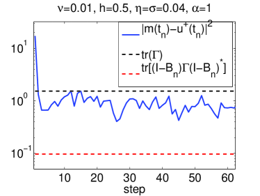
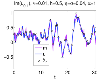
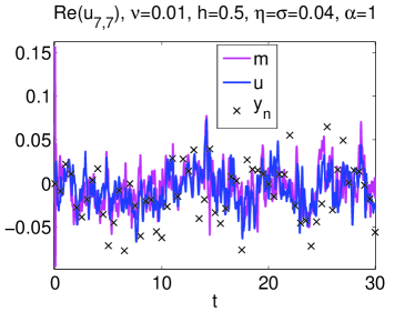
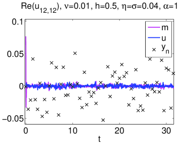
Figure 1: Example of a stable trajectory for 3DVAR with $\nu=0.01,h=0.5,\eta=\sigma=0.04,\alpha=1$. The top left plot shows the norm-squared error between the estimated mean, $m(t_{n})=\hat{m}_{n}$, and the signal, $u(t_{n})$, in comparison to the preferred upper bound (i.e. the total observation error ${\rm tr}(\Gamma)=\Xi$) and the lower bound ${\rm tr}[(I-B_{n})\Gamma(I-B_{n})]$. The other three plots show the estimator, $m(t)$, together with the signal, $u(t)$, and the observations, $y_{n}$ for a few individual modes.

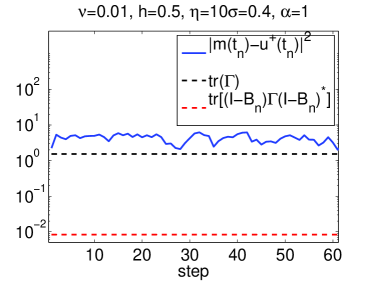
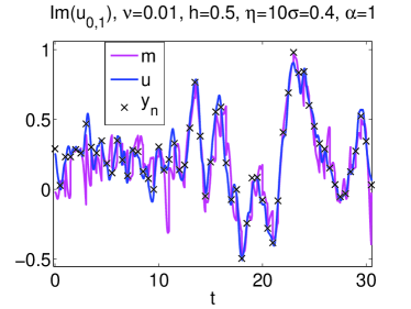
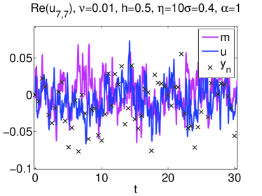
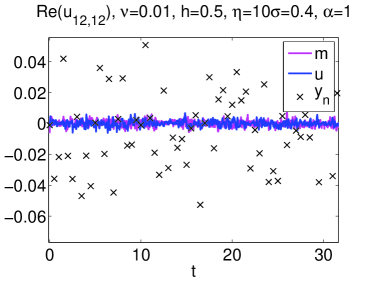
Figure 2: Example of a destabilized trajectory for 3DVAR with the same parameters as in Fig. 1 except the larger value of $\eta=10\sigma=0.4$. Panels are the same.

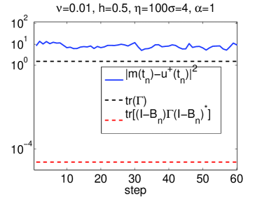
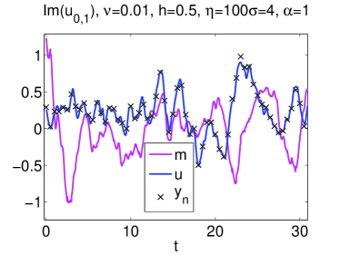
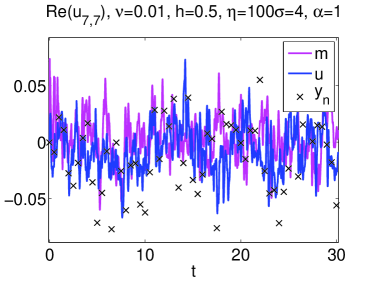
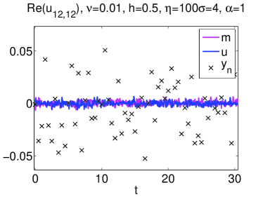
Figure 3: Example of a destabilized trajectory for 3DVAR with the same parameters as in Fig. 1 except the larger value of $\eta=100\sigma=4$. Panels are the same.

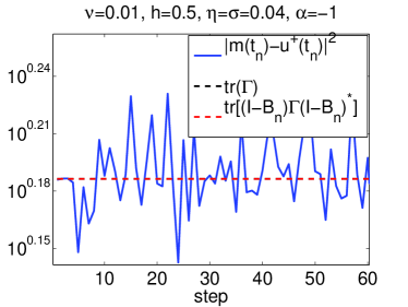
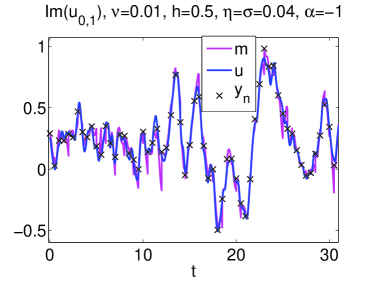
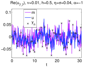
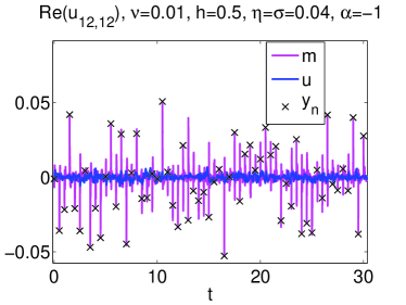
Figure 4: Example of a stable trajectory for 3DVAR with the same parameters as in Fig. 1 except with $\alpha=-1$. Panels are the same.

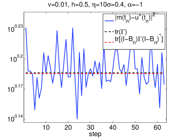
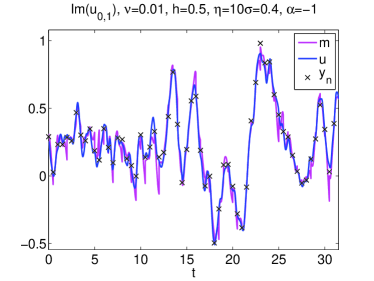
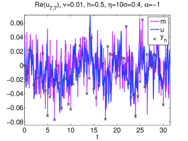
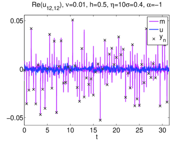
Figure 5: Example of a stable trajectory for 3DVAR with the same parameters as in Fig. 2 except with value of $\alpha=-1$. Panels are the same.

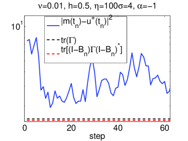
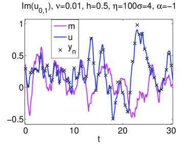
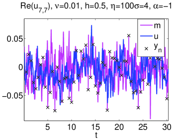
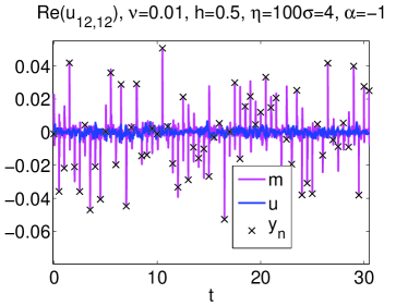
Figure 6: Example of a destabilized trajectory for 3DVAR with the same parameters as in Fig. 3 except with value of $\alpha=-1$. Panels are the same.

4.4 Partial Observations

We now proceed to examine the case of partial observations, illustrating Theorem 3.3. Note that the forced mode has magnitude $|k_{f}|^{2}=50$, so ensuring that it is observed requires that $\lambda>50\lambda_{1}$. When enough modes are retained, for example when $\lambda=100\lambda_{1}$ in our setting, the results for the $\alpha=1$ case remain roughly the same and are not shown. However, in the case $\alpha=-1$, in which the observations are trusted more than the model at high wavevectors, the results are greatly improved by ignoring the observations of the high-frequencies. See Fig. 7. This improvement, and indeed the improvement beyond setting $B=0$ for both cases $\alpha=\pm 1$ disappears as $\lambda$ is decreased. In particular, when $\lambda=25\lambda_{1}$ the error is never very much smaller than the upper bound. This is due to the fact that the dynamics of the low wavevectors tend to be unpredictable and they contain very little useful information for the assimilation. Then, for much smaller $\lambda=4\lambda_{1}$, once enough unstable modes are left unobserved, there is no convergence. The order of magnitude of the error in the asymptotic regime as a function of $\eta$ remains roughly consistent as $\lambda$ is decreased until the estimator no longer converges. For small $h$ (high-frequency in time observations) and complete observations, the estimator can be slow to converge to the asymptotic regime. In this case, the number of iterations until convergence, for a sufficiently small $\eta$, becomes significantly larger as $\lambda$ is decreased (again until the estimator fails to converge at all).

Given $\lambda\approx k_{\lambda}^{2}\lambda_{1}$, we expect that for $\eta$ sufficiently small the contribution of the model to the filter will be negligible for all $k$ with $|k|<k_{\lambda}$ for $\alpha=1$. Hence the estimators for both $\alpha=\pm 1$ will behave similarly. An example of this is shown in Fig. 8 where $\eta=0.01\sigma=0.0004$ and $\lambda=49\lambda_{1}$ in Fig. 8. In both cases, the estimator is essentially utilizing all the available observations. There are enough observations to draw the higher wavevectors of the estimator closer to the truth than if we just set the population of those modes to zero. In contrast, as mentioned above, when $\lambda=25\lambda_{1}$, there are not enough observations even when they are all used, and the error is roughly the same as the upper bound as $\eta\rightarrow 0$ (not shown).

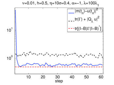
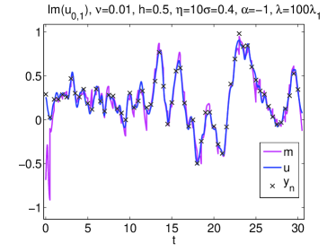
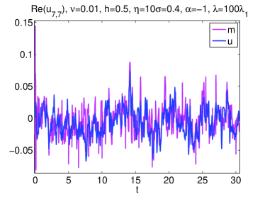
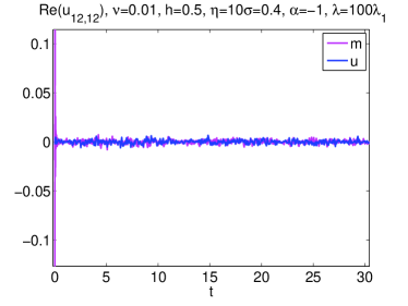
Figure 7: Example of an improved estimator for partial observations with $\lambda=100\lambda_{1}$ and otherwise the same parameters as in Fig. 5. Panels are the same.

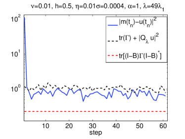
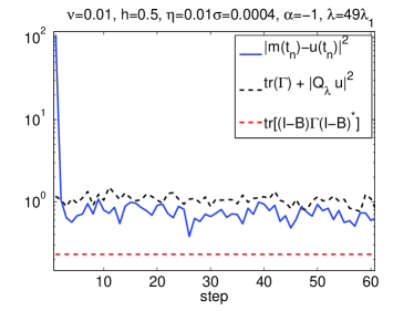
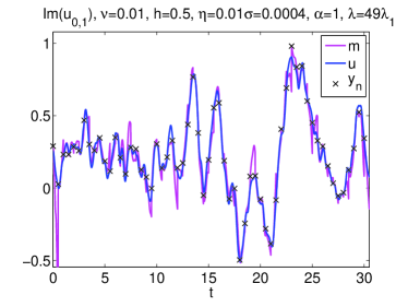
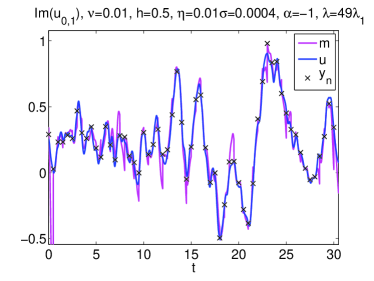
Figure 8: Examples of estimators for partial observations with $\lambda=49\lambda_{1}^{2}$ and $\eta=0.1\sigma=0.004$, otherwise the same parameters as in Figs. 1 and 4. Left panels are for $\alpha=1$ and right panels are for $\alpha=-1$.

5 Conclusion

This paper contains three main components:

• we show that the filtering problem for the Navier-Stokes equation may be formulated as a a sequence of well-posed inverse problems: Theorem 2.3;

• we prove Theorems 3.3 and 3.7, which establish filter accuracy and stability provided variance inflation is employed;

• we describe numerical results which illustrate, and extend the validity of, the theory.

We note that the analysis will also apply to other semilinear dissipative PDEs which possess a squeezing property (contraction when projected into the high modes) and a global attractor; such equations are studied in depth in [25], and include the Cahn-Allen and Cahn-Hilliard equations, the Kuramoto-Sivashinsky equation and Ginzburg-Landau equation. These two structural properties of the underlying model, when combined with sufficient variance inflation ($\eta$ small enough in 3DVAR) enable proof that the 3DVAR filter has a contractive property, even when the underlying dynamical system itself has positive Lyapunov exponents.

There are a number of natural future directions which stem from this work:

• to develop analogous filter stability theorems for more sophisticated filters, such as the extended and ensemble-based methods, when applied to the Navier-Stokes equation;

• to study model-data mismatch by looking at filter stability for data generated by forward models which differ from those used to construct the filter;

• to study the effect of filtering in the presence of model error, by similar methods, to understand how this may be used to overcome problems arising from model-data mismatch.

• to combine the analysis in this paper, which concerns nonlinear problems, but assumes that the observation operator and the Stokes operator commute, and the recent work [27] which concerns only linear autonomous problems but does not assume commutativity of the solution operator for the forward model and the observation operator.

Acknowledgements AMS would like to thank the following institutions for financial support: EPSRC, ERC, ESA, and ONR; KJHL was supported by EPSRC, ESA, and ONR; and CEAB, KFL, DSM and MRS were supported EPSRC, through the MASDOC Graduate Training Centre at Warwick University. The authors also thank The Mathematics Institute and Centre for Scientific Computing at Warwick University for supplying valuable computation time. Finally, the authors thank Masoumeh Dashti for valuable input.

References

- [1] A. C. Lorenc, Analysis methods for numerical weather prediction, Quart. J. R. Met. Soc. 112 (474) (2000) 1177–1194.
- [2] D. F. Parrish, J. C. Derber, The national meteorological center’s spectral statistical-interpolation analysis system, Monthly Weather Review 120 (8) (1992) 1747–1763.
- [3] A. C. Lorenc, S. P. Ballard, R. S. Bell, N. B. Ingleby, P. L. F. Andrews, D. M. Barker, J. R. Bray, A. M. Clayton, T. Dalby, D. Li, T. J. Payne, F. W. Saunders, The Met. Office global three-dimensional variational data assimilation scheme, Quart. J. R. Met. Soc. 126 (570) (2000) 2991–3012.
- [4] P. Courtier, E. Andersson, W. Heckley, D. Vasiljevic, M. Hamrud, A. Hollingsworth, F. Rabier, M. Fisher, J. Pailleux, The ECMWF implementation of three-dimensional variational assimilation (3d-Var). I: Formulation, Quart. J. R. Met. Soc. 124 (550) (1998) 1783–1807.
- [5] Z. Toth, E. Kalnay, Ensemble forecasting at NCEP and the breeding method, Monthly Weather Review 125 (1997) 3297.
- [6] G. Evensen, Data Assimilation: the Ensemble Kalman Filter, Springer Verlag, 2009.
- [7] P. Van Leeuwen, Particle filtering in geophysical systems, Monthly Weather Review 137 (2009) 4089–4114.
- [8] J. Harlim, A. Majda, Filtering nonlinear dynamical systems with linear stochastic models, Nonlinearity 21 (2008) 1281.
- [9] A. Majda, J. Harlim, B. Gershgorin, Mathematical strategies for filtering turbulent dynamical systems, Dynamical Systems 27 (2) (2010) 441–486.
- [10] A. Harvey, Forecasting, Structural Time Series Models and the Kalman filter, Cambridge Univ Pr, 1991.
- [11] A. Doucet, N. De Freitas, N. Gordon, Sequential Monte Carlo methods in practice, Springer Verlag, 2001.
- [12] A. Bain, D. Crişan, Fundamentals of Stochastic Filtering, Springer Verlag, 2008.
- [13] T. Snyder, T. Bengtsson, P. Bickel, J. Anderson, Obstacles to high-dimensional particle filtering, Monthly Weather Review. 136 (2008) 4629–4640.
- [14] P. van Leeuwen, Nonlinear data assimilation in geosciences: an extremely efficient particle filter, Quarterly Journal of the Royal Meteorological Society 136 (653) (2010) 1991–1999.
- [15] A. Chorin, M. Morzfeld, X. Tu, Implicit particle filters for data assimilation, Communications in Applied Mathematics and Computational Science (2010) 221.
- [16] T. Tarn, Y. Rasis, Observers for nonlinear stochastic systems, Automatic Control, IEEE Transactions on 21 (4) (1976) 441–448.
- [17] K. Law, A. Stuart, Evaluating data assimilation algorithms, Arxiv preprint arXiv:1107.4118.
- [18] A. Carrassi, M. Ghil, A. Trevisan, F. Uboldi, Data assimilation as a nonlinear dynamical systems problem: Stability and convergence of the prediction-assimilation system, Chaos: An Interdisciplinary Journal of Nonlinear Science 18 (2008) 023112.
- [19] A. TREVISAN, L. PALATELLA, Chaos and weather forecasting: The role of the unstable subspace in predictability and state estimation problems, International Journal of Bifurcation and Chaos 21 (12) (2011) 3389.
- [20] E. Olson, E. Titi, Determining modes for continuous data assimilation in 2D turbulence, Journal of statistical physics 113 (5) (2003) 799–840.
- [21] K. Hayden, E. Olson, E. Titi, Discrete data assimilation in the Lorenz and 2d Navier-Stokes equations, Physica D: Nonlinear Phenomena.
- [22] P. Constantin, C. Foiaş, Navier-Stokes equations, University of Chicago Press, 1988.
- [23] R. Temam, Navier-Stokes Equations and Nonlinear Functional Analysis, no. 66, Society for Industrial Mathematics, 1995.
- [24] J. C. Robinson, Infinite-Dimensional Dynamical Systems, Cambridge Texts in Applied Mathematics, Cambridge University Press, Cambridge, 2001.
- [25] R. Temam, Infinite-Dimensional Dynamical Systems in Mechanics and Physics, 2nd Edition, Vol. 68 of Applied Mathematical Sciences, Springer-Verlag, New York, 1997.
- [26] C. Brett, K. Lam, K. Law, D. McCormick, M. Scott, A. Stuart, Stability of filters for the Navier-Stokes equation, Arxiv preprint arXiv:1110.2527.
- [27] R. Potthast, A. Moodey, A. Lawless, P. van Leeuwen, On error dynamics and instability in data assimilation, Preprint.
- [28] D. Blömker, K. Law, A. Stuart, K. Zygalakis, Accuracy and stability of the continuous time 3dvar filter for the navier-stokes equation, In preparation.
- [29] S. Cox, P. Matthews, Exponential time differencing for stiff systems, Journal of Computational Physics 176 (2) (2002) 430–455.
- [30] J. Hesthaven, S. Gottlieb, D. Gottlieb, Spectral Methods for Time-Dependent Problems, Vol. 21, Cambridge Univ Pr, 2007.
- [31] A. Majda, X. Wang, Non-linear dynamics and statistical theories for basic geophysical flows, Cambridge Univ Pr, 2006.