Scaling, Finite Size Effects, and Crossovers of the Resistivity and Current-Voltage Characteristics in Two-Dimensional Superconductors

Abstract

We revisit the scaling properties of the resistivity and the current-voltage characteristics at and below the Berezinskii-Kosterlitz-Thouless transition, both in zero and nonzero magnetic field. The scaling properties are derived by integrating the renormalization group flow equations up to a scale where they can be reliably matched to simple analytic expressions. The vortex fugacity turns out to be dangerously irrelevant for these quantities below $T_{c}$, thereby altering the scaling behavior. We derive the possible crossover effects as the current, magnetic field or system size is varied, and find a strong multiplicative logarithmic correction near $T_{c}$, all of which is necessary to account for when interpreting experiments and simulation data. Our analysis clarifies a longstanding discrepancy between the finite size dependence found in many simulations and the current-voltage characteristics of experiments. We further show that the logarithmic correction can be avoided by approaching the transition in a magnetic field, thereby simplifying the scaling analysis. We confirm our results by large scale numerical simulations, and calculate the dynamic critical exponent $z$, for relaxational Langevin dynamics and for resistively and capacitively shunted Josephson junction dynamics.

Fluctuation effects can be very strong in low-dimensional systems and may radically alter the mean field picture of phase transitions. A well known example is that of two-dimensional (2D) superfluids or superconductors, where phase fluctuations of the complex order parameter $\psi=\psi_{0}e^{i\theta}$ destroy long range order at all nonzero temperatures. Despite this, a superfluid/superconducting phase with algebraic order, finite superfluid stiffness, and zero resistivity, still exists at low temperature. This is separated from the high temperature disordered phase by a transition – the Berezinskii-Kosterlitz-Thouless (BKT) transition – caused by the thermal unbinding of vortex-antivortex pairs Berezinskii (1971); *Berezinskii2; Kosterlitz and Thouless (1973); Minnhagen (1987). The properties of 2D superconductors have been studied intensely in recent years Repaci et al. (1996); *Herbert1998; *MiuMiu2006; *Mondal2011; *Baturina; Strachan et al. (2003) and continue to receive much interest due to the relevance for cuprate superconductors with their layered structure. Furthermore, advances in fabrication enable studies of single or few atomic layer thick superconductors, which offer great potential for precise tests against theories and simulations Reyren et al. (2007); *Logvenov2009; *Ye2010. In this paper we explore the possible scaling behaviors and crossover effects that may occur as a function of current, magnetic field, and system size. These results are confirmed by numerical simulations and used for an accurate determination of the dynamic critical exponent for two different equations of motion.

Transport measurements are perhaps the best way to experimentally study the properties of 2D superconductors. One of the hallmarks of the BKT transition is the nonlinear current-voltage (IV) characteristics $E\sim J^{a(T)}$ at and below $T_{c}$, with a temperature dependent exponent $a(T)$ Ambegaokar et al. (1978); *AHNS2; Halperin and Nelson (1979). The exact form of the temperature dependence of the exponent $a(T)$ has been subject to some debate Minnhagen et al. (1995). According to the conventionally accepted theory developed by Ambegaokar, Halperin, Nelson and Siggia (AHNS), $a(T)=a_{\text{AHNS}}=1+2\pi\mathcal{J}(T)/2T$, where $\mathcal{J}(T)=\hbar^{2}\rho_{s}(T)/2m$ is the superfluid stiffness and $\rho_{s}(T)$ the (fully renormalized) superfluid areal density Ambegaokar et al. (1978); *AHNS2; Halperin and Nelson (1979). This result has been contested by Minnhagen et al. (MWJO) Minnhagen et al. (1995) who arrived at the alternative expression $a(T)=a_{\text{MWJO}}=2\pi\mathcal{J}(T)/T-1$ using scaling arguments. Both yield $a=3$ at the transition $T_{c}=\pi\mathcal{J}(T)/2$. Alternatively one may try to describe the data using a Fisher-Fisher-Huse (FFH) scaling formula Fisher et al. (1991)

$$E=J\xi^{d-2-z}\mathcal{E}(J\xi^{d-1}/T),$$ (1)

where $\mathcal{E}(\cdot)$ is a scaling function and $\xi$ the correlation length. This leads also to a power-law, but leaves $a=z+1$ as a free fitting parameter related to the dynamic critical exponent $z$ ($d=2$ is the dimension). In 2D, however, fits of experimental data to Eq. (1) easily give surprisingly large values $a\gtrsim 6$ Pierson et al. (1999), although more reasonable values $\approx 3$ have also been obtained Strachan et al. (2003). This, however, highlights the difficulty in using Eq. (1) without additional assumptions. In any case it remains challenging to decide which of the scenarios described above is correct based only on experiments. One may instead resort to computer simulations to try to settle the controversy. Usually, simulation data are analyzed using finite size scaling formulas based on Eq. (1), with the diverging correlation length $\xi$ cut off by the system size $L$, yielding $E\sim JL^{1-a}$ for small $J$. Most Medvedyeva et al. (2000); Kim et al. (1999); Jensen et al. (2000); Minnhagen et al. (2004); Weber et al. (1996) (but not all Simkin and Kosterlitz (1997); Chen et al. (2001); *TangChen) simulation studies appear to favor the value $a_{\text{MWJO}}$. Interestingly, Refs. Chen et al., 2001; *TangChen, obtain agreement with both the AHNS and MWJO expressions in different regimes and for different boundary conditions. At the same time, the validity of the FFH scaling formula Eq. (1) is still an open question, as is the scaling behavior in the presence of an applied magnetic field.

The main contribution to the scaling behavior of the resistivity and IV characteristics comes from the free vortex density $n_{F}$ of unbound vortex pairs. These can be either thermally excited or induced by an applied magnetic field or a current. Since only the motion of free vortices dissipate energy, the resistivity should be proportional to the free vortex density

$$\rho=\Phi_{0}^{2}\mu_{v}n_{F},$$ (2)

where $\Phi_{0}$ is the flux quantum and $\mu_{v}\approx 2\pi\xi_{0}^{2}\rho_{n}/\Phi_{0}^{2}$ is the Bardeen-Stephen vortex mobility.

Conventionally, the free vortex density $n_{F}=n_{F}^{+}+n_{F}^{-}$ is calculated from a rate equation Ambegaokar et al. (1978); *AHNS2

$$\frac{dn_{F}^{\pm}}{dt}=\Gamma-\lambda n_{F}^{+}n_{F}^{-},$$ (3)

where $\Gamma=\lambda\zeta^{2}e^{-U_{\text{eff}}/T}$ is the pair generation rate and $\lambda$ the recombination rate. Here $\zeta=e^{-E_{c}/T}$ is the vortex fugacity, and $E_{c}\sim\mathcal{J}$ the vortex core energy. The potential barrier to overcome in order to create a pair of free vortices has two terms, one which depends logarithmically on their separation $r$, and one with a linear dependence due to the applied current $U_{\text{eff}}(r)\approx 2\pi\mathcal{J}\ln(r/a_{0})-J\Phi_{0}r$, where $a_{0}\approx\xi_{0}$ is a short distance cutoff of the order of the Ginzburg-Landau coherence length. (From now on we set $a_{0}=1$.) Optimizing gives $r^{*}\approx 2\pi\mathcal{J}/\Phi_{0}J$ and $U_{\text{eff}}=U_{\text{eff}}(r^{*})\approx-2\pi\mathcal{J}\left[\ln(J\Phi_{0}a_{0}/2\pi\mathcal{J})+1\right]$. The stationary solution to Eq. (3) gives

$$n_{F}=2\zeta e^{-U_{\text{eff}}/2T}\sim 2\zeta J^{2\pi\mathcal{J}/2T},$$ (4)

and, with $E=\rho(J)J$, the result $a=a_{\text{AHNS}}$.

There are several ways in which the above picture may need to be modified. First, interactions between vortices except those constituting the pair are completely neglected. Screening of the vortex interaction from bound vortex-antivortex pairs can be taken into account by using the fully renormalized value of the stiffness $\mathcal{J}(T)$ in place of the bare one. In a finite system the vortices may enter and exit the system at the boundaries and Eq. (3) will acquire more terms describing these processes. Accounting for a realistic geometry and nonuniform current distribution can lead to a rather complicated behavior Gurevich and Vinokur (2008). In simulations one usually avoids surface effects by using periodic boundary conditions (PBC). Finite size effects, however, become visible when $r^{*}=2\pi\mathcal{J}/\Phi_{0}J\gtrsim L$, leading to a crossover to ohmic behavior at low currents, with a characteristic size dependent resistivity. Another issue is that the rate equation (3) presumes that density fluctuations are small, which is true for large systems, but not for small enough systems with area $L^{2}\lesssim 1/n_{F}$. In the latter regime the constraint of vortex-antivortex neutrality (enforced when using PBC ) instead leads to $\Gamma/\lambda=\left<{n_{F}^{+}n_{F}^{-}}\right>\approx\left<{n_{F}^{\pm}}\right>^{2}+L^{-2}\left<{n_{F}^{\pm}}\right>$, which is dominated by the second term, i.e.,

$$n_{F}\sim 2L^{2}\zeta^{2}e^{-U_{\text{eff}}/T},\quad(\text{PBC and }L^{2}n_{F}\lesssim 1).$$ (5)

The same expression follows from a low fugacity expansion of the neutral Coulomb gas, which only involves even powers of $\zeta$. Also note that an applied perpendicular magnetic field $B$ will lead to a net density of free vortices $\Delta n=n_{F}^{+}-n_{F}^{-}=B/\Phi_{0}$, such that

$$n_{F}^{2}={\Delta n^{2}+4n_{F}^{+}n_{F}^{-}}\approx{\Delta n^{2}+4\zeta^{2}e^{-U_{\text{eff}}/T}}.$$ (6)

A more systematic approach to take into account interaction effects, is to first integrate the renormalization group (RG) flow up to the scale where one of the coupling constants becomes large of $O(1)$ and only then match the theory to simple approximate expressions similar to the ones discussed above. The RG flow equations are most easily expressed in the Coulomb gas language using the rescaled temperature and fugacity variables, $x=1-\frac{\pi\mathcal{J}}{2T}$, $y=2\pi\zeta$. To lowest order in $x$ and $y$ they read Kosterlitz (1974); Minnhagen (1987)

$$\frac{dx}{d\ell} =2y^{2}, \frac{dy}{d\ell} =2xy,$$ (7)

where $\ell=\ln b$ is the logarithm of the scale factor $b$. The resulting RG flow obeys $x^{2}-y^{2}=C^{2}$, where

$$|C|=\sqrt{|x_{0}^{2}-y_{0}^{2}|}\approx c\sqrt{|T_{c}-T|}$$ (8)

is a constant determined by the initial conditions. Below $T_{c}$ we have $C^{2}>0$ and the RG flow ends up on a critical line $x=-C<0$, $y=0$ as $\ell\to\infty$. Above $T_{c}$, $C^{2}<0$ and the flow will eventually diverge to $+\infty$. The BKT transition occurs at $T=T_{c}$, where the flow follows the separatrix $x=-y$. In order to describe the various crossovers we need the explicit solutions Kosterlitz (1974), $y(\ell)=C/{\sinh(2C(\ell-\ell_{0}))}$ for $T<T_{c}$, $y(\ell)=1/{(2\ell-2\ell_{0})}$ for $T=T_{c}$, and $y(\ell)=-{|C|}/{\sin(2|C|(\ell-\ell_{0}))}$ for $T>T_{c}$. In terms of $b=e^{\ell}$ we have

$$y(b) =\frac{2C(b/b_{0})^{-2C}}{1-(b/b_{0})^{-4C}}, (T<T_{c}),$$ (9)

$$y(b) =\frac{1}{2\ln(b/b_{0})}, (T=T_{c}),$$ (10)

where $b_{0}=e^{\ell_{0}}$ is fixed by the initial conditions. Near $T_{c}$, where $|C|\lesssim y_{0}$, we have to a good approximation $c^{2}\approx 4y_{0}/\pi\mathcal{J}$, $T_{c}\approx\pi\mathcal{J}/2(1+y_{0})$, $\ell_{0}\approx-1/2y_{0}$. Further below $T_{c}$, where $C\gtrsim y_{0}$, we have instead $C\approx-x_{0}$, so that

$$y(b) \approx y_{0}b^{-2C}, (T\ll T_{c}).$$ (11)

Note also that $C=-x(b\to\infty)=\pi\mathcal{J}_{R}(T)/2T-1$ is directly related to the fully renormalized superfluid stiffness $\mathcal{J}_{R}(T)$.

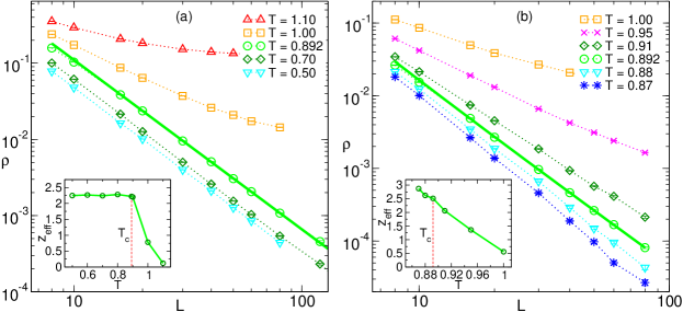
Figure 1: (Color online) Langevin dynamics. (a) Resistivity $\rho$ vs system size $L$ at different temperatures in a magnetic field $B=\Phi_{0}/L^{2}$. The dotted lines are guides for the eyes, and the full green curve at $T=T_{c}$ is a $\chi^{2}$-fit (using $L=16$–$120$) to the power-law $\rho\sim L^{-z}$, giving $z=2.22$. (b) As in (a), but for zero magnetic field. The full green curve at $T=T_{c}$ is a $\chi^{2}$-fit (using $L=16$–$80$) to $\rho\sim L^{-2.22}/(\ln L-\ell_{0})^{2}$ with fixed $z=2.22$, giving $\ell_{0}=-2.71$. Insets: The effective exponent $z_{\text{eff}}$ vs temperature, obtained from power-law fits. Note how $z_{\text{eff}}$ is almost constant below $T_{c}$ in (a).

The free vortex density, being the vortex density which remains after the elimination of all bound pairs, is only rescaled by the RG transformation and therefore has scaling dimension 2, i.e, $n_{F}\sim b^{-2}$. As a function of system size $L$, magnetic flux density $B$, current $J$, $x$, $y$, and possibly other perturbations it therefore transforms as

$$n_{F}(x_{0},y_{0},L,B,J,\ldots)=\\ b^{-2}n_{F}(x(b),y(b),Lb^{-1},Bb^{2},Jb,\ldots)$$ (12)

under the RG. A similar equation holds for the resistivity Eq. (2). Most theories assume that the vortices undergo ordinary diffusion However, we are not aware of any argument which prevents the renormalization of the vortex mobility $\mu_{v}$ in Eq. (2). Hence, we allow for an anomalous dimension $\mu_{v}\sim b^{2-z}$, with a dynamic critical exponent $z$ not necessarily fixed to 2, such that the resistivity transforms as

$$\rho(x_{0},y_{0},L,B,J,\ldots)=\\ b^{-z}\rho(x(b),y(b),Lb^{-1},Bb^{2},Jb,\ldots).$$ (13)

An FFH scaling formula follows from Eq. (13) if $\rho$ flows smoothly to a nonzero constant as $b\to\infty$. This is the case above $T_{c}$, where the flow must be stopped at a scale when $x\sim y\sim O(1)$, yielding the Debye-Hückel expression $n_{F}\approx 1/2\pi\xi_{+}^{2}$, where $\xi_{+}\sim\exp({\pi/2c\sqrt{T-T_{c}}})$ is the correlation length above $T_{c}$. This is, however, not the case in zero magnetic field at and below $T_{c}$, where $y=2\pi\zeta\to 0$, because $n_{F}$ vanishes in this limit. In other words, the fugacity is dangerously irrelevant for $n_{F}$ and $\rho$ in this case. Instead the right hand side of Eqs. (12)-(13) must be matched to one of Eqs. (4)-(6). At the matching scale $b$ the barrier $U_{\text{eff}}$ in Eq. (4) or (5) has reduced to zero, and we are left with three different possibilities: In zero magnetic field $n_{F}(b)\sim y(b)$ or $y^{2}(b)$ depending on boundary conditions and system size, while for nonzero field $n_{F}(b)\approx\sqrt{B^{2}b^{4}/\Phi_{0}^{2}+y^{2}(b)/\pi^{2}}$. This will turn out to have profound consequences for the scaling of many quantities.

We first discuss the finite size scaling of the linear resistivity in zero magnetic field. The RG flow must then be stopped at $b=L$. Under the RG all length scales, including the system size, shrink by a factor $b$ so that the effective system size becomes $L^{\prime}=L/b=1$. The system must therefore be matched to Eq. (5) when using periodic boundary conditions, or to (4) when using open boundary conditions. For PBC we thus get $\rho(L)\sim L^{-z}y^{2}(L)$, and by using Eqs. (9)-(11), the limiting cases

$$\rho(L)\sim\begin{cases}L^{-z+4-2\pi\mathcal{J}_{R}/T},&(L\gtrsim\xi_{-}),\\ L^{-z}/\ln^{2}(L/b_{0}),&(L\lesssim\xi_{-}),\end{cases}$$ (14)

where $\xi_{-}\approx\exp({1/2C})\approx\exp({1/2c\sqrt{T_{c}-T}})$ is the correlation length below $T_{c}$, defined as the scale on which $x(b)$ has approximately reached its asymptotic value $-C$. The power-law appearing in this expression agrees with the finite size scaling of MWJO Medvedyeva et al. (2000) if one assumes $z=2$. On the other hand, for open boundary conditions $\rho(L)\sim L^{-z}y(L)$, or

$$\rho(L)\sim\begin{cases}L^{-z+2-\pi\mathcal{J}_{R}/T},&(L\gtrsim\xi_{-}),\\ L^{-z}/\ln(L/b_{0}),&(L\lesssim\xi_{-}),\end{cases}$$ (15)

which, for $z=2$, would be consistent with the AHNS scaling. The finite size scaling at $T_{c}$, where $\xi_{-}=\infty$, has in both cases, strong multiplicative logarithmic corrections.

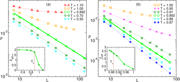
Figure 2: (Color online) Overdamped RCSJ dynamics (Stewart-McCumber $\beta_{C}=2\pi I_{c}R^{2}C/\Phi_{0}=0.25$). (a) Resistivity $\rho$ vs system size $L$ at different temperatures in a magnetic field $B=\Phi_{0}/L^{2}$. The full green curve at $T=T_{c}$ is a $\chi^{2}$-fit (using $L=16$–$120$) to the power-law $\rho\sim L^{-z}$, giving $z=1.77$. (b) As in (a), but for zero magnetic field. The full green curve at $T=T_{c}$ is a $\chi^{2}$-fit (using $L=16$–$80$) to $\rho\sim L^{-1.77}/(\ln L-\ell_{0})^{2}$ with fixed $z=1.77$, giving $\ell_{0}=-1.33$. Insets: As in Fig. 1.

The situation in a nonzero magnetic field is different. The magnetic field is a relevant perturbation, which destroys superconductivity by introducing a finite density of free vortices even at low temperature. We can, however, still approach the transition by scaling down the magnetic field with the system size, holding $BL^{2}=N\Phi_{0}$, the net number of flux quanta, fixed. (This is easy in a simulation, but more difficult in an experiment.) Consider, e.g., the case $N=1$. Stopping the RG flow at $b\sim L=\sqrt{\Phi_{0}/B}$ and matching to Eq. (6) then gives $\rho\sim L^{-z}\sqrt{1+y^{2}(L)/\pi^{2}}$. The leading scaling behavior thus remains a temperature independent power-law with exponent $z$ in contrast to the zero field case (with a weak additive correction decreasing with system size).

The finite size scaling formulas derived above are well-suited for the analysis of numerical simulations. We have performed simulations of the 2D XY model, defined by the Hamiltonian $H=-\mathcal{J}\sum_{\left<{ij}\right>}\cos(\theta_{i}-\theta_{j}-A_{ij})$, using two types of dynamics, relaxational Langevin dynamics and resistively and capacitively shunted Josephson junction (RCSJ) dynamics (in the overdamped limit) [Detailsofthesimulationmethodscanbefoundin]Andersson2011. The resistivity was calculated from the equilibrium voltage fluctuations using a Kubo formula, with a sampling time of $10^{6}$–$10^{8}$ time units per datapoint. For an accurate determination of $z$ we apply a weak magnetic field $B=\Phi_{0}/L^{2}$ so that the system contains exactly one vortex irrespective of system size. This minimizes the influence of the logarithmic correction near $T_{c}$, allowing us to fit the data for $T\leq T_{c}$ to the simple scaling law $\rho(L)\sim L^{-z}$. We plot, in Fig. 1(a), $\rho$ vs $L$ calculated using Langevin dynamics on a log-log scale for a range of temperatures including $T_{c}$ ($T_{c}\approx 0.892\mathcal{J}$ Olsson (1995)). The data at and below $T_{c}$ do indeed follow a power-law with a temperature independent exponent $z\approx 2.22\pm 0.05$. In contrast, the zero field data shown in Fig. 1(b) follow different power-laws at different temperatures. Right at $T_{c}$ the data is very well fitted by Eq. (14) with $z$ fixed to $2.22$. The value of $\ell_{0}=\ln b_{0}\approx-2.7$ obtained by the fit compares well with the theoretical estimate $\ell_{0}\approx-1/2y_{0}\approx-2$ obtained using the XY value $y_{0}=2\pi e^{-E_{c}/T}$, with $E_{c}\approx\pi^{2}\mathcal{J}/2$. Without knowing about the logarithmic correction one would fit the data at $T_{c}$ to a pure power-law and draw the wrong conclusion. For our data this would give an effective exponent $z_{\text{eff}}\approx 2.54$, appreciably different from the true $z$.

Figure 2 shows similar plots for RCSJ dynamics. The resistivity for a system with exactly one vortex again follows a power-law, but this time with $z=1.77\pm 0.05$ at $T_{c}$. In zero field the data is well fitted to (14) using the same $z$, with $\ell_{0}\approx-1.33$ again in rough agreement with expectations, whereas a pure power-law fit would give a too large exponent $z_{\text{eff}}\approx 2.2$.

The values $z\approx 2.22$ and $z\approx 1.77$ for Langevin and RCSJ dynamics, respectively, are close to, but significantly different from the conventional value 2, and correspond either to subdiffusive ($z>2$) or superdiffusive ($z<2$) vortex motion.

The scaling behavior below $T_{c}$ differs considerably in zero and nonzero magnetic field. As seen in the insets of Figs. 1 and 2 the resistivity with $B=\Phi_{0}/L^{2}$ follows a power law with practically temperature-independent exponents in stark contrast to the zero field case. Previous finite size scaling studies of $\rho(L)$ (or $E(J,L)$ in the ohmic regime) in zero field have obtained a temperature-dependent power-law exponent below $T_{c}$ in good agreement with the MWJO prediction Kim et al. (1999); Jensen et al. (2000); Minnhagen et al. (2004); Weber et al. (1996); Chen et al. (2001); *TangChen, which is not surprising given (14) and the smallness of $z-2$.

In a large or infinite system at zero magnetic field, the RG flow must be stopped at a scale dictated by the applied current, i.e., when $Jb\approx J_{0}=2\pi\mathcal{J}/\Phi_{0}$. At this scale the matching condition is $n_{F}\sim y$ and the nonlinear resistivity $\rho(J)\sim J^{z}y(b\approx J_{0}/J)$ obtains from Eqs. (9)-(11). We have the limiting cases

$$\rho(J)=\frac{E}{J}\sim\begin{cases}J^{z+\pi\mathcal{J}_{R}(T)/T-2},\quad&J_{0}/J\gtrsim\xi_{-},\\ J^{z}/\ln(J_{0}/Jb_{0}),\quad&J_{0}/J\lesssim\xi_{-}.\end{cases}$$ (16)

The power-law behavior at low currents below $T_{c}$ is in agreement with the AHNS value if one assumes $z=2$. Close to $T_{c}$ we find a strong multiplicative logarithmic correction. The crossover to the finite size induced ohmic behavior in Eq. (14) or (15) happens when $JL\lesssim J_{0}$. In addition one expects a high-current crossover to an ohmic regime when $J\gtrsim J_{0}$.

In the PBC case it is also possible to have an intermediate regime where the matching is still done at a scale $b\approx J_{0}/J$, but the effective system size is small enough that $n_{F}(b)(L/b)^{2}\lesssim 1$, so that $n_{F}\sim y^{2}$. This would give

$$\rho(J,L) \sim L^{2}J^{z-2+2\pi\mathcal{J}_{R}/T}, \frac{J_{0}}{J}\lesssim L\lesssim\left(\frac{J_{0}}{J}\right)^{\pi\mathcal{J}_{R}/2T}\!\!\!\!\!\!\!\!\!.$$ (17)

Such an intermediate scaling regime was previously proposed in Ref. Chen et al., 2001; *TangChen, using an entirely different approach.

To summarize, we have obtained a coherent picture of the scaling behavior and crossover effects of the (nonlinear) resistivity near and below the BKT transition, Eqs. (14)–(17). The finite size results depend sensitively on the boundary conditions and on whether a magnetic field is present or not. In the limit of large systems the IV exponent agrees with the AHNS result, with the modification that we allow for the possibility that $z\neq 2$. For PBC, on the other hand, the finite size scaling agrees with MWJO. Our simulations suggest that $z$ differs from $2$ and moreover that Langevin and RCSJ dynamics belong to different dynamic universality classes Hohenberg and Halperin (1977). From a practical point we found it important to take into account the logarithmic correction near $T_{c}$ when analyzing finite size data. The same should hold true for experimental finite current data. Note, however, that to make quantitative comparisons with experiments it may be important to consider effects of inhomogeneity and pinning, and to make realistic estimates of the temperature dependence of the bare parameters $\mathcal{J}$, $y$, e.g., using Ginzburg-Landau theory Benfatto et al. (2009). Finally, it should be noted that the only assumptions needed in our analysis is the low fugacity behavior of the zero magnetic field resistivity $\rho\sim y$ or $y^{2}$. It is highly likely that other quantities may be affected in similar ways.

We thank M. Wallin for comments on the manuscript. This work was supported by the Swedish Research Council (VR) through grant no. 621-2007-5138 and the Swedish National Infrastructure for Computing (SNIC 001-10-155) via PDC.

References

- Berezinskii (1971) V. S. Berezinskii, Sov. Phys. JETP 32, 493 (1971).
- Berezinskii (1972) V. S. Berezinskii, Sov. Phys. JETP 34, 610 (1972).
- Kosterlitz and Thouless (1973) J. M. Kosterlitz and D. J. Thouless, J. Phys. C 6, 1181 (1973).
- Minnhagen (1987) P. Minnhagen, Rev. Mod. Phys. 59, 1001 (1987).
- Repaci et al. (1996) J. M. Repaci, C. Kwon, Q. Li, X. Jiang, T. Venkatessan, R. E. Glover, C. J. Lobb, and R. S. Newrock, Phys. Rev. B 54, R9674 (1996).
- Herbert et al. (1998) S. T. Herbert, Y. Jun, R. S. Newrock, C. J. Lobb, K. Ravindran, H.-K. Shin, D. B. Mast, and S. Elhamri, Phys. Rev. B 57, 1154 (1998).
- Miu et al. (2006) L. Miu, D. Miu, G. Jakob, and H. Adrian, Phys. Rev. B 73, 224526 (2006).
- Mondal et al. (2011) M. Mondal, S. Kumar, M. Chand, A. Kamlapure, G. Saraswat, G. Seibold, L. Benfatto, and P. Raychaudhuri, Phys. Rev. Lett. 107, 217003 (2011).
- Baturina et al. (2012) T. I. Baturina, S. V. Postolova, A. Y. Mironov, A. Glatz, M. R. Baklanov, and V. M. Vinokur, EPL (Europhysics Letters) 97, 17012 (2012).
- Strachan et al. (2003) D. R. Strachan, C. J. Lobb, and R. S. Newrock, Phys. Rev. B 67, 174517 (2003).
- Reyren et al. (2007) N. Reyren, S. Thiel, A. D. Caviglia, L. F. Kourkoutis, G. Hammerl, C. Richter, C. W. Schneider, T. Kopp, A.-S. Rüetschi, D. Jaccard, M. Gabay, D. A. Muller, J.-M. Triscone, and J. Mannhart, Science 317, 1196 (2007).
- Logvenov et al. (2009) G. Logvenov, A. Gozar, and I. Bozovic, Science (New York, N.Y.) 326, 699 (2009).
- Ye et al. (2010) J. T. Ye, S. Inoue, K. Kobayashi, Y. Kasahara, H. T. Yuan, H. Shimotani, and Y. Iwasa, Nature materials 9, 125 (2010).
- Ambegaokar et al. (1978) V. Ambegaokar, B. I. Halperin, D. R. Nelson, and E. D. Siggia, Phys. Rev. Lett. 40, 783 (1978).
- Ambegaokar et al. (1980) V. Ambegaokar, B. I. Halperin, D. R. Nelson, and E. D. Siggia, Phys. Rev. B 21, 1806 (1980).
- Halperin and Nelson (1979) B. I. Halperin and D. R. Nelson, JLTP 36, 599 (1979).
- Minnhagen et al. (1995) P. Minnhagen, O. Westman, A. Jonsson, and P. Olsson, Phys. Rev. Lett. 74, 3672 (1995).
- Fisher et al. (1991) D. S. Fisher, M. P. A. Fisher, and D. A. Huse, Phys. Rev. B 43, 130 (1991).
- Pierson et al. (1999) S. W. Pierson, M. Friesen, S. M. Ammirata, J. C. Hunnicutt, and L. A. Gorham, Phys. Rev. B 60, 1309 (1999).
- Medvedyeva et al. (2000) K. Medvedyeva, B. J. Kim, and P. Minnhagen, Phys. Rev. B 62, 14531 (2000).
- Kim et al. (1999) B. J. Kim, P. Minnhagen, and P. Olsson, Phys. Rev. B 59, 11506 (1999).
- Jensen et al. (2000) L. M. Jensen, B. J. Kim, and P. Minnhagen, Phys. Rev. B 61, 15412 (2000).
- Minnhagen et al. (2004) P. Minnhagen, B. J. Kim, and A. Grönlund, Phys. Rev. B 69, 064515 (2004).
- Weber et al. (1996) H. Weber, M. Wallin, and H. J. Jensen, Phys. Rev. B 53, 8566 (1996).
- Simkin and Kosterlitz (1997) M. V. Simkin and J. M. Kosterlitz, Phys. Rev. B 55, 11646 (1997).
- Chen et al. (2001) Q.-H. Chen, L.-H. Tang, and P. Tong, Phys. Rev. Lett. 87, 067001 (2001).
- Tang and Chen (2003) L.-H. Tang and Q.-H. Chen, Phys. Rev. B 67, 024508 (2003).
- Gurevich and Vinokur (2008) A. Gurevich and V. M. Vinokur, Phys. Rev. Lett. 100, 227007 (2008).
- Note (1) By PBC we mean, here and in the following, any boundary condition which enforces vortex neutrality.
- Kosterlitz (1974) J. M. Kosterlitz, Journal of Physics C: Solid State Physics 7, 1046 (1974).
- Andersson and Lidmar (2011) A. Andersson and J. Lidmar, Phys. Rev. B 83, 174502 (2011).
- Olsson (1995) P. Olsson, Phys. Rev. B 52, 4526 (1995).
- Hohenberg and Halperin (1977) P. C. Hohenberg and B. I. Halperin, Rev. Mod. Phys. 49, 435 (1977).
- Benfatto et al. (2009) L. Benfatto, C. Castellani, and T. Giamarchi, Phys. Rev. B 80, 214506 (2009).