The clustering of intermediate redshift quasars as measured by the Baryon Oscillation Spectroscopic Survey
Abstract
We measure the quasar two-point correlation function over the redshift range using data from the Baryon Oscillation Spectroscopic Survey. We use a homogeneous subset of the data consisting of 27,129 quasars with spectroscopic redshifts—by far the largest such sample used for clustering measurements at these redshifts to date. The sample covers 3,600, corresponding to a comoving volume of assuming a fiducial CDM cosmology, and it has a median absolute -band magnitude of , -corrected to . After accounting for redshift errors we find that the redshift space correlation function is fit well by a power-law of slope and amplitude Mpc over the range Mpc. The projected correlation function, which integrates out the effects of peculiar velocities and redshift errors, is fit well by a power-law of slope and Mpc over the range Mpc. There is no evidence for strong luminosity or redshift dependence to the clustering amplitude, in part because of the limited dynamic range in our sample. Our results are consistent with, but more precise than, previous measurements at similar redshifts. Our measurement of the quasar clustering amplitude implies a bias factor of for our quasar sample. We compare the data to models to constrain the manner in which quasars occupy dark matter halos at and infer that such quasars inhabit halos with a characteristic mass of with a duty cycle for the quasar activity of 1 per cent.
1 Introduction
Quasars are among the most luminous astrophysical objects, and are believed to be powered by accretion onto supermassive black holes (e.g. Salpeter, 1964; Lynden-Bell, 1969). They have become a key element in our current paradigm of galaxy evolution – essentially all spheroidal systems at present harbor massive black holes (Kormendy & Richstone, 1995), the masses of which are correlated with many properties of their host systems. The emerging picture is that quasar activity and star formation are inextricably linked (e.g. Nandra et al., 2007; Silverman et al., 2008) in galaxies that contain a massive bulge (and thus a massive black hole) and a gas reservoir. The galaxy initially forms in a gas-rich, rotation-dominated system. Once the dark matter halo grows to a critical scale some event—most likely a major merger (Carlberg, 1990; Haiman & Loeb, 1998; Cattaneo, Haehnelt & Rees, 1999; Kauffmann & Haehnelt, 2000; Springel et al., 2005; Hopkins et al., 2006) or instability in a cold-stream fed disk (Ciotti & Ostriker, 1997, 2001; Di Matteo et al., 2012)—triggers a period of rapid, obscured star formation and the generation of a stellar bulge. After some time the quasar becomes visible, and soon after the star formation is quenched on a short timescale, perhaps via radiative or mechanical feedback from the central engine (e.g. Shankar, 2009; Natarajan, 2012; Alexander & Hickox, 2012).
The clustering of quasars as a function of redshift and luminosity provides useful constraints on our understanding of galaxy evolution. The large-scale clustering amplitude increases with the mass of the dark matter halos hosting the quasars. Comparison of the abundance of such halos to that of quasars can provide constraints on the duty cycle and degree of scatter in the observable halo-mass relation (Cole & Kaiser, 1989; Martini & Weinberg, 2001; Haiman & Hui, 2001; White, Martini & Cohn, 2008; Shankar, Weinberg & Shen, 2010). However quasars are extremely rare, so very large surveys are necessary to suppress the shot-noise from Poisson fluctuations. Samples of quasars have only recently included enough objects to study their clustering with some precision (Porciani, Magliocchetti & Norberg, 2004; Croom et al., 2005; Porciani & Norberg, 2006; Hennawi et al., 2006a; Myers et al., 2006, 2007a, 2007b; da Angela et al., 2008; Padmanabhan et al., 2009; Ross et al., 2009; Shen et al., 2009).
Naively, measuring the clustering of quasars between redshift 2 and 3 should be a simple task, as this is where the comoving number density of luminous quasars seemingly peaks (Weedman, 1986; Hartwick & Schade, 1990; Croom et al., 2005; Richards et al., 2006). However, selection effects complicate quasar targeting in this range. The colours of normal (unobscured) quasars around resemble far more abundant stellar populations, particularly metal-poor A and F halo stars (e.g., Fan, 1999; Richards et al., 2001). This issue is enhanced at the faint limits of imaging surveys that achieve similar depth to the Sloan Digital Sky Survey (SDSS; York et al., 2000), where those compact galaxies that are dominated by A and F stellar populations contaminate selection at the 10–20 per cent level as star-galaxy separation becomes difficult (e.g., Richards et al., 2009; Bovy et al., 2012). In addition, faint quasars with –2.6 can have similar colours to quasars at , which are contaminated by redder light from their host galaxy (e.g., Budavári et al., 2001; Richards et al., 2001; Weinstein et al., 2004). In combination, the cuts that must be made to efficiently select quasars in this redshift range mean that optical surveys of quasars may miss a significant number of quasars. A wide-area survey at high targeting density is thus an attractive proposition for the study of quasar clustering at moderate redshift. The data we consider in this paper are drawn from just such a survey; the Baryon Oscillation Spectroscopic Survey (BOSS; Eisenstein et al., 2011).
Physical effects also conspire to make quasars difficult to sample at . Obviously, quasars simply appear fainter at greater distances, but in addition quasars seem to exhibit cosmic downsizing, with the population of less luminous quasars peaking at lower redshift (Croom et al., 2009). Thus, the most luminous quasars are both more abundant and the most visible members of the quasar population at . Quasar clustering measurements at high redshift from the original SDSS (Shen et al., 2007) therefore only sample the most luminous quasars, implying that deeper spectroscopy than used for the original SDSS quasar survey (Richards et al., 2002a) is necessary for sampling quasars across a large dynamic range in luminosity near . Indeed, the final BOSS quasar sample should be larger, and almost 2 magnitudes deeper, than the original SDSS spectroscopic quasar sample at (14,065 objects; Schneider et al., 2010).
The outline of the paper is as follows. In §2 we describe the quasar samples that we use—drawn from the SDSS and the BOSS. The clustering measurements are described in §3, including comparisons with earlier work. The implications of our results for quasars are explored in §4. We conclude in §5. Appendix A discusses the impact of redshift errors on our measurements while Appendix B contains the technical details of the model fits used in this paper. Where necessary we shall adopt a CDM cosmological model with , and as assumed in White et al. (2011), Anderson et al. (2012) and Reid et al. (2012). Unless the dependence is explicitly specified or parametrized, we assume . Dark matter halo masses are quoted as , i.e. the mass interior to a radius within which the mean density is the background density of the Universe. Luminosities will be quoted in Watts, and magnitudes in the AB system.
2 Data
The Sloan Digital Sky Survey (SDSS; York et al., 2000) mapped nearly a quarter of the sky using the dedicated Sloan Foundation 2.5-meter telescope (Gunn et al., 2006) located at Apache Point Observatory in New Mexico. A drift-scanning mosaic CCD camera (Gunn et al., 1998) imaged the sky in five photometric bandpasses (Fukugita et al., 1996; Smith et al., 2002; Doi et al., 2010) to a limiting magnitude of . The imaging data were processed through a series of pipelines that perform astrometric calibration (Pier et al., 2003), photometric reduction (Lupton et al., 2001), and photometric calibration (Padmanabhan et al., 2008). We use quasars selected from this 5-band SDSS photometry as described in detail in Bovy et al. (2011) and Ross et al. (2012).
Selecting quasars in the redshift range –3, where the space density of the brightest quasars peaks (Richards et al., 2006; Croom et al., 2009), is made difficult by the large populations of metal-poor A and F stars, faint lower redshift quasars and compact galaxies which have similar colours to the objects of interest (e.g., Fan, 1999; Richards et al., 2001). In our case the problem is compounded by the fact that we wish to work close to the detection limits of the SDSS photometry, where errors on flux measurements cause objects to scatter substantially in colour space, and that the BOSS key science programs did not include the study of the clustering of quasars.
2.1 Clustering subsamples and the angular mask
The quasar component of BOSS is designed primarily as a Lyman- Forest survey, which does not require quasars to be selected in a uniform—or even a recreatable—manner across the sky. For the study of quasar clustering however, uniform selection is key. To satisfy these competing scientific requirements, the survey thus adopted a CORE+BONUS strategy, where the CORE objects correspond to a uniform sample selected by the extreme deconvolution (XD)111XD (Bovy et al., 2009) is a method to describe the underlying distribution function of a series of points in parameter space (e.g., quasars in colour space) by modeling that distribution as a sum of Gaussians convolved with measurement errors. algorithm. XD is applied in BOSS to model the distributions of quasars and stars in flux space, and hence to separate quasar targets from stellar contaminants (XDQSO; Bovy et al., 2011). It is this CORE sample that we analyze in this paper.
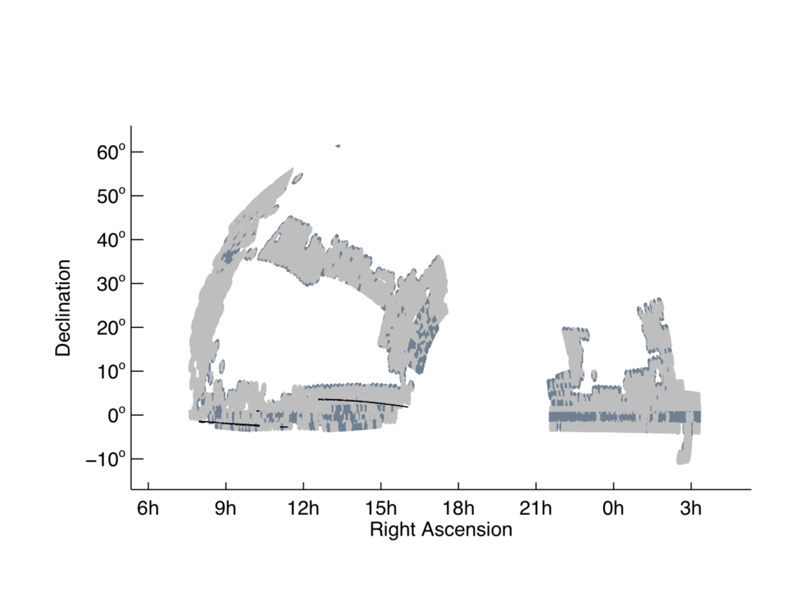
Specifically, we take as quasar targets all point sources in SDSS imaging that have an XDQSO probability above a threshold of to the magnitude limit of BOSS quasar target selection ( or ; Ross et al., 2012). By quasar targets in this sense, we mean all quasars that would have been observed in a perfect survey. In reality, not all such targets are observed because not all fibers can be placed on an object during normal survey operations. More importantly, the XDQSO algorithm was not adopted as the final CORE algorithm for BOSS quasar target selection until the second year of operations (Ross et al., 2012). We will work with spectroscopy take on or before January 1, 2012—just over the first two years of BOSS data. So, on average, more potential targets with an XDQSO probability greater than are unobserved (spectroscopically) in areas that were covered in the first year of BOSS (see Fig. 1).

We use the Mangle software (Swanson et al., 2008) to track the angular completeness of the survey (the mask). The completeness on the sky is determined from the fraction of quasar targets in a sector for which we obtained a spectrum; a sector is an area of the sky covered by a unique set of spectroscopic tiles (see Blanton et al., 2003; Tegmark et al., 2004). For our analyses, we limit the survey to areas with targeting completeness greater than 75 per cent. By targeting completeness, we mean the ratio of the number of quasar targets that received a BOSS fiber to all quasar targets.
We do not correct for spectroscopic incompleteness—i.e. account for the fraction of observed targets which produce a spectrum of sufficient quality to measure a redshift. Quasars at are identifiable in BOSS even at very low signal-to-noise ratio because the strong Ly 1215 line always falls within the BOSS wavelength coverage (3,600–10,000Å; Eisenstein et al., 2011). In BOSS, almost all unidentifiable objects are likely to be stars, galaxies or low redshift quasars, not the quasars of interest in this paper. Correcting for spectroscopic incompleteness would induce a false large scale clustering signal because the density of stellar contaminants varies over the sky.
We apply a veto mask to remove survey regions in which a quasar could never be observed— areas near bright stars and the centerposts of the spectroscopic plates (as described in White et al., 2011). We also remove fields where the conditions were not deemed photometric by the SDSS imaging pipeline (again see White et al., 2011). Finally, we remove areas that have bad data in the SDSS imaging scans (§3.3 of Abazajian et al., 2004, see Fig. 1). The resulting XDQSO CORE targets were matched to the list of objects for which the BOSS successfully obtained a spectrum, and throughout this paper we only consider regions where at least 75 per cent of the XDQSO CORE targets received a BOSS fiber for spectroscopic observation.
We study BOSS data taken on or before January 1, 2012. This limits our analysis to version 5_5_0 of the spectral reduction pipeline (spAll-v5_5_0) and to the areas plotted in Fig. 1. Note that these are slightly later reductions than made publicly available with SDSS Data Release 9 (DR9; which uses v5_4_45). Algorithmically v5_5_0 is the same as v5_4_45, but changes for calibrations of a newly installed CCD affects data past DR9.
2.2 Redshift assignation
The BOSS wavelength coverage is 3,600–10,000Å so for quasars above the [O III] 4958,5007 complex is shifted out of the BOSS window. Systemic redshifts for most BOSS quasars thus rely solely on information from broad emission lines in the rest-frame ultraviolet. The next lowest ionization line typically found in quasar spectra Mg II 2798, which is a good redshift indicator (Richards et al., 2002b), is shifted entirely beyond the BOSS spectral coverage near . To measure quasar redshifts above we rely on combinations of the C III 1908, C IV 1549, and Ly 1215 lines. In addition to being broad, the centroid of each line may be biased—C III] is often blended with Si III], Al III and Fe III complexes, C IV can be shifted from the systemic redshift by strong outflows, and Ly is often affected by Ly Forest absorption and is blended with NV (e.g., Vanden Berk et al., 2001; Richards et al., 2002b, 2011).
To ameliorate these issues, when the BOSS pipeline222The BOSS pipeline is described in Aihara et al. (2011) identifies a quasar spectrum as having an Mg II, C III] or C IV line that is within the BOSS wavelength coverage, we default to the redshift from that line offset using the prescription of Hewett & Wild (2010). For spectra with no such lines, we adopt the BOSS pipeline redshift. The BOSS collaboration is visually inspecting all quasar spectra to check the pipeline redshifts. When a pipeline redshift conflicts with the visual redshift (438 objects) we adopt the human-corrected redshift. As we mainly analyze clustering on scales that correspond to velocities that are larger than typical quasar broad lines, altering redshifts by a small amount does not strongly affect our results. Appendix A discusses redshift errors further.
2.3 Quasar luminosities and k-corrections
Fig. 2 plots the conditional magnitude distribution of our sample, compared to the characteristic luminosity of quasars at that redshift. We correct all magnitudes to using the -corrections derived by Richards et al. (2006). The characteristic luminosity—where the luminosity function changes slope—from Croom et al. (2004), as modified by Croton (2009), is
| (1) |
where and for and and for . We have converted from the band used by Croom et al. (2004) to the -band (-corrected to ) using (Richards et al., 2006). Note that in the range , which will be the focus of this paper, we are able to probe 1–2 magnitudes fainter than the characteristic magnitude.
| Sample | Name | Redshift | Magnitude | |
|---|---|---|---|---|
| 1 | All | 27,129 | ||
| 2 | Bright | 13,564 | ||
| 3 | Dim | 13,564 | ||
| 4 | Fid | 19,111 | ||
| 5 | LoZ | 8,835 | ||
| 6 | HiZ | 9,977 |
Using SDSS broad-band colours to derive -corrections for our sample is problematic. Most BOSS quasars at redshift are near the flux limit of SDSS imaging, and so they have noisier colours than for previous SDSS prescriptions at brighter limits (e.g. Richards et al., 2006). Deriving full -corrections at as a function of flux, colour and redshift is beyond the scope of this paper (but see McGreer et al. 2012, in preparation). Precise -corrections will require proper modeling of subtle changes due to, e.g., the Baldwin Effect, the presence of complex iron emission crossing through the -band, and the movement of broad lines—which can be offset due to luminosity-and-redshift-dependent winds and absorption features—across the SDSS filter set. For the redshifts on which we focus in this paper () only the C III 1908 line enters the -band. Fortuitously, this complex does not shift much with luminosity, which reduces any flux dependence to the -correction for our sample.
3 Clustering
All of our clustering measurements are performed in configuration, rather than Fourier, space. For rare objects, where shot-noise is an important or dominant piece of the error budget, the configuration space estimators have the advantage of more nearly independent errors. They also deal well with irregularly-sampled geometries, such as we have for our sample. We shall compute both the real- and redshift-space correlation functions, using the Landy & Szalay (1993) estimator, with a density of random points times the density of quasars.
3.1 The random catalog
As discussed in §2.1 we use Mangle (Swanson et al., 2008) to track the angular completeness of the survey. Angular positions for the random points, modulated by the angular completeness of the survey, were obtained from the Mangle program ransack. To assign redshifts to the random catalog we tried three methods, which yielded almost identical results. The first was to assign to each point a redshift drawn at random from the data. While this method would produce artificial structure in the redshift distribution of the random points for a small survey, due to sample variance, the wide angular coverage of the BOSS survey ensures this method performs well. We also tried fitting splines to the histogram of the quasar redshifts and the cumulative histogram of the redshifts and using those splines to generate random redshifts. The results were insensitive to using the histogram or cumulative histogram, to the number of spline points and to the type of spline used. For the results presented below we use the first method.
3.2 Fiber collisions and small-scale clustering
We cannot obtain spectroscopic data for a few percent of quasars due to fiber collisions—no two BOSS fibers can be placed closer than on a specific plate. At the exclusion corresponds to Mpc (comoving). Where possible we obtain redshifts for the collided quasars in regions where plates overlap. We account for the remaining exclusions by restricting our analyses to relatively large scales and by up-weighting quasar-quasar pairs with separations smaller than . The upweighting is derived by comparing the angular correlation function of all targets with that of the quasars for which we obtained redshifts (Hawkins et al., 2003; Li et al., 2006; Ross et al., 2007; White et al., 2011). This ratio is close to unity above but drops to about two-thirds below . The number of pairs for which this correction is appreciable is quite small, and the impact of this correction is much less than even on the smallest scales. If fiber-collided quasars preferentially live in regions of higher-than-average density the large-scale clustering would be affected by fiber collisions and would not be properly corrected by our weighting procedure. The efficiency of the tiling algorithm, the prioritization of quasar targets over galaxies and the depth of the survey combine to make fiber collisions a very small effect on our analysis (see also Ross et al., 2009).


3.3 Tests of systematics
We have performed numerous jackknife tests to check whether our results are robust to possible systematics. Specifically we have investigated whether our results are stable to cuts on targeting, at what point in the survey the plates were drilled and what targeting algorithm was used, sector completeness, Galactic latitude and hemisphere (Fig. 3), extinction in the -band, target areal density, stellar density, raw -band magnitude (which is a proxy for signal-to-noise ratio), sky brightness, -band seeing (Fig. 4) and selection threshold. In all cases but one we see no evidence for a statistically significant systematic effect. The exception is that there is weak evidence that the large-scale clustering of quasars in the South Galactic Cap is stronger than that in the North Galactic Cap. It will require more data to determine whether this is a statistical fluctuation or a significant difference—and, of course, we conducted eleven, not one, different tests of systematics. When eleven (independent) trials are performed the likelihood of a 2 detection is quite high ( per cent instead of per cent for a single trial). In future a quasar catalog with good photometric redshifts could help with some of these issues. In addition BOSS will continue to obtain quasar data until 2014, so we defer a more detailed investigation of geographical discrepancies to a future publication.

3.4 Clustering results
We have insufficient sensitivity to measure the angular dependence of the redshift-space clustering induced by redshift space distortions for our highly biased quasars. Therefore, we only quote redshift-space results from the angle-averaged correlation function, which we denote at redshift space separation . Real-space clustering is constrained by the projected correlation function
| (2) |
avoiding the need to model redshift space distortions and mitigating any effects of redshift errors. We truncate the integral over the line-of-sight separation, , to Mpc. This value represents a trade-off between the goal of fully integrating out the effects of redshift space distortions and the disadvantages of introducing noise from only weakly correlated structures along the line-of-sight and mixing a wide range of 3D scales into a single bin. By Mpc the effects of redshift space distortions are negligible, and the truncation has only a modest effect on our largest scale point. However this truncation must be kept in mind when precise modeling of the data at the largest is important (see below).
| 4.36 | 5.19 | 6.17 | 7.34 | 8.72 | 10.37 | 12.34 | 14.67 | |
|---|---|---|---|---|---|---|---|---|
| 42.87 | 24.18 | 32.12 | 23.21 | 23.98 | 21.13 | 16.25 | 16.80 | |
| 17.08 | 10.89 | 10.77 | 8.36 | 9.85 | 7.12 | 6.16 | 4.08 | |
| 4.36 | 1.000 | 0.459 | 0.156 | 0.125 | 0.187 | 0.154 | -0.198 | -0.146 |
| 5.19 | – | 1.000 | 0.210 | 0.094 | 0.261 | 0.032 | -0.256 | -0.019 |
| 6.17 | – | – | 1.000 | 0.341 | -0.029 | 0.118 | 0.168 | 0.173 |
| 7.34 | – | – | – | 1.000 | 0.069 | 0.404 | -0.113 | -0.076 |
| 8.72 | – | – | – | – | 1.000 | 0.004 | 0.053 | 0.091 |
| 10.37 | – | – | – | – | – | 1.000 | -0.107 | -0.119 |
| 12.34 | – | – | – | – | – | – | 1.000 | 0.251 |
| 14.67 | – | – | – | – | – | – | – | 1.000 |

We divide our quasar sample into bins of redshift over which the bias and mass correlation function are evolving strongly. Fortuitously, on the scales of relevance the effects approximately cancel, i.e. the clustering amplitude stays approximately constant. The redshift-bin-averaged can be approximated as a measurement of evaluated at an effective redshift, :
| (3) |
so that
| (4) |
where is the redshift distribution of the sample, is the Hubble parameter at redshift and is the comoving angular diameter distance to redshift (Matarrese et al., 1997; White, Martini & Cohn, 2008). Assuming passive evolution, constant halo mass, or constant bias leads to differences between and that are far smaller than our observational errors.


Results for each of the samples in Table 1 are shown in Figs. 5 and 6, and the values for the full sample, with and no cuts on magnitude, are given in Table 2. Both the real- and redshift-space clustering are fit well by a model with an underlying power-law correlation function, once the effects of projection and redshift errors are taken into account. As it provides a good fit to the data, and for consistency with earlier work (e.g. Myers et al., 2006; Ross et al., 2009; Shen, 2009), we shall show lines in the figures and provide fits in the tables assuming a power-law slope of for the real-space correlation function. The actual slope of the correlation function is poorly determined by the projected correlation function data. Power-law indices from to are viable. The best-fit slope is quite shallow, near . The value of at Mpc for the best-fit model is almost independent of the assumed slope.
We estimate the covariance matrix of our measurements by bootstrap resampling (e.g. Efron & Gong, 1983). We divide the survey into angular regions specified by HealPix pixels (Gorski et al., 2005) with (i.e. approximately on a side). Pixels which contain fewer random points than two-thirds of the mean are merged with higher occupancy pixels to ensure pixels have similar weight. We then estimate both the mean and covariance matrix by bootstrap resampling pair counts from a random draw of pixels (with replacement).
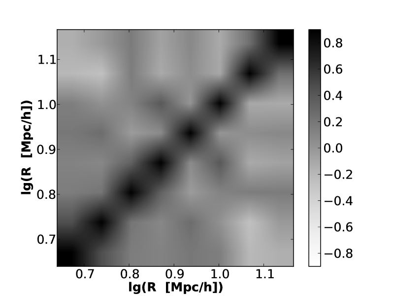
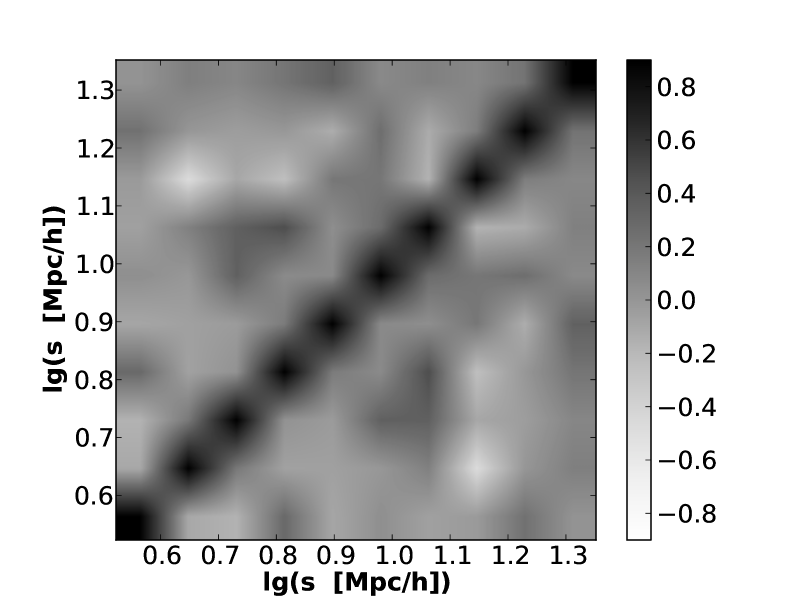
The bootstrap-determined correlation matrices for the full sample for and are shown in Figs. 7 and 8 respectively. Note that the matrices are diagonal-dominated as might be expected for shot-noise limited measurements—extending to larger scales we see larger correlations between the bins, most notably in . As we begin to restrict the quasar sample in redshift or luminosity, and the number of objects becomes smaller, the covariance matrices and their inverses can become increasingly noisy. We have several options at this point—with the most desirable being a reduction in the number of degrees of freedom (i.e. data-compression) so that we can apply bootstrap resampling to obtain a converged covariance matrix, or error on a summary statistic (or statistics). The simplest approach would be to reduce the number of bins so that we have fewer, better constrained points. However this is not optimal for our purposes. We describe below a different approach based on the sparsity of our sample and the nature of the clustering.
To begin we note that the correlation functions are fit well ( for 7 degrees of freedom for , and for 9 degrees of freedom for ) by power-laws over the range where our constraints are tightest (as expected if quasars are hosted by massive halos, see Fig. 9). We adopt a two parameter model for both and of the form and
| (5) |
which corresponds to a 3D correlation of the form integrated to along the line-of-sight. For the prefactor is and we shall fix throughout so that we have one remaining degree of freedom. We fit these models to the measured correlations over the range Mpc and Mpc. The non-linear, scale-dependent bias of dark matter halos makes their correlation functions close to a power-law on Mpc scales (see Figs. 9 and 10) but at larger scales the bias becomes scale-independent and the correlation functions drop more quickly than the power-law extrapolation would suggest. In addition, on larger scales sample variance becomes increasingly important and the radial bins become increasingly correlated (especially for ). For these reasons we limit the fitting range as indicated (see also Croom et al., 2005). With more data and a numerical model for the covariance matrix we could extend the range of the measurement and tighten the constraints on quasar models.
For a power-law correlation function of fixed slope each point provides an estimate of the correlation length, , since . The number of pairs in a bin of fixed is and if shot-noise dominates the bins are independent and the fractional error on in each bin scales as . Thus, assuming logarithmic bins and that shot-noise dominates we can average the estimates with inverse variance weights so that
| (6) |
where the weights are
| (7) |
The values of depend on an estimate, , for , and reduce to
| (8) |
Most of the weight in the fit is produced by , with the weight scaling as for small and for large . Since the bins are assumed to be logarithmically spaced, for this suppression is quite rapid in both directions, reflecting the paucity of pairs at small and the weakness of the correlation signal at large . If the correlation function continued as a power-law to large we could tighten our constraints by extending the fitting range, but it is at these larger scales where deviations from a power-law behavior are most expected, and where the correlations between measurements in adjacent radial bins act to weaken the constraints.
Unfortunately, it is difficult to find a precise redshift for quasars in the range from optical spectroscopy, so our correlation function is smeared by redshift errors which reduce the small-scale clustering signal (the dotted lines in Fig. 6; Appendix A discusses the impact of redshift uncertainties further). We include redshift errors in our model through a multiplicative factor, , derived in Appendix A. The best fit can be derived from a generalization of Eq. (6) which replaces the weights with , multiplies the in the weights by and divides each term in the numerator of Eq. (6) by .
For a given estimate, , the optimal estimate of can be written either as a weighted sum of the bins or directly in terms of the pair counts themselves. One can iterate this estimator, in which case the error properties of become more complex and are best handled by a bootstrap procedure. We generate for each bootstrap sample, with the iterative weighting scheme above starting from , and use the standard deviation for our estimate of uncertainty. This uncertainty estimate does not include the additional contribution from our uncertainty in the redshift error correction. A change in redshift error () of per cent moves the best-fit by , which can be considered an additional systematic error on the fit. While a 25 per cent uncertainty on the redshift error is consistent with Appendix A, we find that reasonable fits to can be obtained for a wide range of redshift error due to a degeneracy between the assumed redshift error and the amplitude (and slope) of the underlying correlation function. Because of this additional uncertainty, our strongest cosmological constraints will come from the projected correlation function, to which we now turn.
A similar estimator can be used for the real-space correlation length, , under the same assumptions. The weights in this case become if the integration in Eq. 2 extends from to . For the weights are nearly constant for all the samples we consider for all of interest. As for the case of the redshift errors and , we can account for the effects of finite on Eq. 5 by modifying the weights to and dividing each term in the numerator by , where333Assuming that is large enough that fingers-of-god are correctly included and so that the anisotropy due to redshift-space distortions is small. for .
The clustering strength derived from this procedure is a statistically valid summary of the data under the assumption that a power-law provides a good fit to . However it does not need to be an optimal compression of the available information — if the data are sufficiently informative a better constraint on the clustering amplitude could be obtained by fitting all of the data. For the full sample (#1 in Table 1), where we have a reasonably converged estimate for the covariance matrix, we can compare the different methods. In this case, the likelihood derived from the determined as above is very similar to that derived from the full covariance matrix (or the diagonal elements) indicating that in our case our estimate of does provide an almost exhaustive summary of the constraints available (Fig. 11). This will be even more the case for samples with more shot-noise. Our simple estimator is the preferred approach for quoting clustering measurements and errors on sparse samples where estimating a full covariance matrix is not feasible.
In addition to our estimates of and we also provide another summary statistic (motivated by Croom et al., 2005; da Angela et al., 2008; Ross et al., 2009),
| (9) |
with Mpc and Mpc. For Eq. (9) becomes
| (10) | |||||
| (11) |
where the last step assumes . We adopt a lower limit, , to mitigate the effect of redshift errors and scale-dependent bias—Eq. 11 shows that this differs from the case by 25 per cent for a power-law of index . With our lower limit the bias inferred from modeling using the Kaiser (1987) prescription
| (12) |
agrees to 1 per cent with that inferred from the real-space clustering for the simulation results described in Figs. 9 and 10. If is used in place of in Eq. 12, the error is also 1 per cent for the case shown in Figs. 9 and 10, though it becomes larger for more biased samples. We compute from the data by assuming can be modeled as a constant within the 10 bins, spaced equally in log between and . The values are corrected upwards by 7 per cent to account for the effect of redshift errors. To allow easy comparison with earlier work we use the value of to estimate the bias in Table 3.
| Sample | Redshift | Magnitude | Median | Mean | Bias | ||||
|---|---|---|---|---|---|---|---|---|---|
| 1 | |||||||||
| 2 | |||||||||
| 3 | |||||||||
| 4 | |||||||||
| 5 | |||||||||
| 6 |
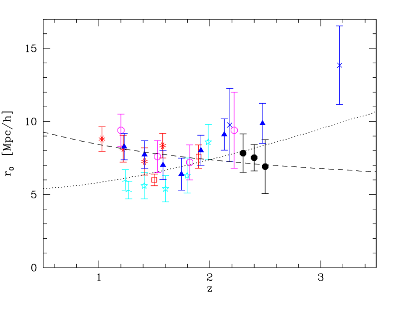
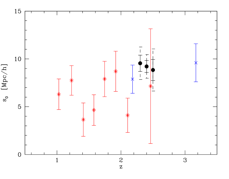
Our results are listed in Table 3 and compared to previous work in Figure 12. We do not detect a luminosity or redshift dependence of the clustering strength, although our sensitivity to this dependence is weak due to the limited dynamic range in both variables in our sample. When comparing to previous work, we do not plot the last 4 points quoted in Table 2 of the SDSS Data Release 5 (DR5 Adelman-McCarthy et al., 2007) quasar clustering analysis of Ross et al. (2009). Due to the flux-limited quasar selection by the original SDSS, the projected measurement for these high- bins are quite noisy (Shen et al., 2007; Ross et al., 2009), and thus unreliable for any direct comparison to our BOSS measurement. We have checked that even if we use the SDSS DR7 data this situation is not improved for our redshift range of interest.
Our results strongly favor the consensus that quasars inhabit rare and highly biased dark matter halos on the exponential tail of the mass function. In the absence of merging we would expect the clustering of such halos to evolve slowly with time. For our assumed cosmology our quasar samples have biases in the range 3.4–4, consistent with early observations and the extrapolation of previous measurements by Croom et al. (2005). Estimates in the literature on the typical halo mass for a bright quasar at comparable redshifts vary wildly, in part due to methodological differences and the fitting functions assumed. So, we now turn to how quasars occupy dark matter halos (see also Appendix B).

4 Interpretation and modeling
One of the main goals of studying quasar clustering is to provide information on the parent dark matter halos hosting luminous quasars. The large-scale bias of the quasars provides information on the mean dark matter halo mass; the small-scale clustering provides information on satellite fractions and potentially radial profiles within halos. Unfortunately the space density of quasars cannot be used directly in such constraints because the quasar duty cycle (or activity time) is not known. This is a major difference with studies of e.g., galaxy clustering, and has serious implications for the constraints that can be derived.
Our median quasar has and so a bolometric luminosity of W (Croom et al., 2005; Shen et al., 2009). If this object is radiating at the Eddington limit (W), then the median in our sample is . As we shall describe, our data are consistent with host halos having a characteristic mass of (Fig. 11), in agreement with earlier work (Porciani, Magliocchetti & Norberg, 2004; Croom et al., 2005; Porciani & Norberg, 2006; Lidz et al., 2006). This value is also consistent with estimates from the relation (Ferrarese, 2002; Fine et al., 2006), , with the differences arising from different assumptions about the halo profiles or data sets. This result suggests , consistent with the results of Croom et al. (2005).
However, we don’t expect quasars to inhabit halos of a single mass (though see Shanks et al., 2011). Constraining the possibly complex manner in which quasars occupy halos from the relatively featureless correlation functions we have access to is difficult, but the modeling is made easier by a number of facts. Quasars are rare, their activity times are short and the fraction of binary quasars is very small444When the virial radius of the hosting halo is much smaller than the mean inter-quasar separation, the fraction of quasar-hosting halos which contain a second quasar scales as , where is the volume averaged correlation function within the virial radius. (Hennawi et al., 2006a; Myers et al., 2007b). This suggests that most quasars live at the center of their dark matter halos and the majority of halos host at most one active quasar. To place constraints on the range of halos in which quasars may be active we consider two illustrative models described below (see Appendix B for further details and De Graf et al. 2011 for a recent discussion in the context of numerical hydrodynamic simulations). To make interpretation easier we use a quasar sample which is limited at both the bright and faint ends, i.e. or (see Table 1, sample #4, “Fid”). We use the measurements listed in Table 3 to constrain the models, though similar results are obtained using the data and its covariance matrix. We also find that the best-fitting models below provide a good fit to the redshift space clustering, assuming our fiducial model for redshift errors.
4.1 Lognormal model
In this model we assume that quasars of some luminosity, , live in halos with a lognormal555Quasars are known to have a relatively high bias and hence live in halos on the steeply falling tail of the mass function. The differences between occupation models which include a high- cut-off and those that do not is therefore relatively small. distribution of masses, centered on a characteristic mass that scales with (see also Appendix B). Each halo hosts at most one quasar with probability
| (13) |
where the normalization is set by the observed space-density of quasars but does not matter for the clustering. We expect that will be larger for more luminous quasars that are hosted by more massive galaxies.
For illustration we assume that the lognormal form holds for quasars in the luminosity bin , i.e. that the luminosity dependence of is weak. This is a reasonable approximation to many models (see Appendix B) and in particular the type described in the next section. We generate quasar samples from halos in the output of 4 cosmological simulations, each employing particles () in a Gpc box. As in Fig. 9, halos are found in the simulations by the friends-of-friends algorithm with a linking length of 0.168 times the mean inter-particle separation. The halos are selected with a lognormal probability centered on a series of . To test for sensitivity to the width of the distribution we consider , 50 and 100 per cent. The former is more appropriate for higher redshift or brighter quasars (White, Martini & Cohn, 2008; Shankar, Weinberg & Shen, 2010; De Graf et al., 2011) while the latter is roughly expected based on the amount of observed scatter in the local relation. We average the projected correlation function for each model—with the same binning and as the data—over the 4 simulations to reduce noise, and compute a goodness-of-fit. Using either the full bootstrap covariance matrix or just the diagonal entries, we find that the best-fit model is good for all choices of . Not surprisingly, we obtain consistent results if we fit to the average of the simulations using the procedure of §3 and then compare to the value in Table 3. Our measurements suggest , 12.05 and 12.15 () for , 50 and 100 per cent, corresponding to an average halo mass ().
The majority of high mass galaxies at high redshift are the central galaxy in their dark matter halo, so observational stellar mass functions can provide constraints on the stellar-to-halo-mass relation at (see Moster et al., 2010; Behroozi, Conroy & Wechsler, 2010, for recent examples). In combination with the constraints on from quasar clustering, and an assumption about the mean Eddington ratio of our sample, we can infer the typical relation for our quasars. Taking the lognormal model and adopting the conversion of Moster et al. (2010), the average stellar mass is –10.2 (with larger values corresponding to larger ). If the accretion occurs at the median black hole mass is using the conversions of (Croom et al., 2005; Shen et al., 2009). We compare these numbers to a variety of published relations in Fig. 13. Our results are in broad agreement with the high redshift inferences but predict larger black holes (at fixed halo mass) than what would be inferred from the local relation of Haring & Rix (2004), even if we assume all of the stellar mass associated with the halo central galaxy is in the bulge and that quasars radiate at Eddington (). This result argues that should increase, at fixed , by a factor of approximately between and . This change is consistent with the increase measured in lensed quasar hosts by Peng et al. (2006) and the model of Hopkins et al. (2007a). By comparison, the model of Croton et al. (2006, Fig. 1) predicts roughly an order of magnitude increase in at between and . On the other hand, the simulations of Sijacki et al. (2007, Fig. 15) predict almost no evolution at the massive end. Merloni et al. (2010) infer evolution of from the zCOSMOS survey with a best-fit power-law of –a factor of 2.3 between and – while Decarli et al. (2010) measure a best-fit power-law of –a factor of 1.4 between and – from a carefully constructed sample of 96 quasars drawn from the literature. Our result favors stronger evolution, but given the statistical and systematic uncertainties in all of the measurements, the uncertainties in stellar mass estimates and selection biases towards more massive black holes in flux-limited surveys all we can say is that it is encouraging that we see evolution in the same sense.
Inverting this argument, we note that, at these high redshifts and masses, obtaining a reasonable relation provides constraints on the possible occupancy distributions of quasars. In particular, because the halo mass function is much steeper than the galaxy stellar mass function, the typical stellar mass of a central galaxy drops steeply with decreasing halo mass—another way of stating that galaxy formation is inefficient in low mass halos. If black-hole properties are set by the galactic potential rather than by halo properties we expect curvature in the relation, which impacts how we interpret the duty cycle or the active quasar fraction.


4.2 Scaling-relation model
Another possibility is that the instantaneous luminosity of the quasar is drawn from a lognormal distribution with central value proportional to a power of the halo mass (or circular velocity) or the central galaxy mass (or dispersion). Physically such a model would arise if quasars radiate with a small range of Eddington ratios and are powered by black holes whose masses are tightly correlated with the mass or circular velocity of the galaxy or host halo (through e.g. black-hole bulge, bulge galaxy and galaxy halo correlations). The lognormal scatter is a combination of the dispersions in each of the relations connecting instantaneous luminosity to halo mass (see e.g. Croton, 2009; Shen, 2009, for recent examples of such models and Appendix B for further references).
We consider two examples here. First we relate the black-hole properties to those of the host halo directly. We choose to use the peak circular velocity of the dark matter halo as our measure of halo size and take to be normally distributed around the (log of)
| (14) |
The normalization, , is set by matching the clustering amplitude at a given luminosity. In principle we can allow the power-law index to vary666For example, an index of would be appropriate to black holes whose growth is stopped by momentum-driven winds and for those whose growth is stopped by luminosity-driven winds (Silk & Rees, 1998).. Unfortunately the range of luminosities we can probe observationally is relatively small and the differences in index are difficult to measure.

For a given and scatter the halo population defines a luminosity function of possible quasars. The comparison of this to the observed luminosity function of active quasars allows us to set the duty cycle, which will be luminosity (and hence halo mass) dependent. For each model we generate a mock catalog drawn from the halos of the simulations introduced in §4.1. We impose the duty cycle by randomly subsampling the possible quasars to ensure the distribution matches the observed luminosity function and then impose the magnitude limits to match the observed sample. We compute and fit for as described previously.
Fig. 14 shows the duty cycle for the best-fit model with . The duty cycle peaks near one per cent at , corresponding to or black hole masses of . This is near the center of our magnitude range and in our model corresponds to halos of several times or . Converting the duty cycle into an activity time is somewhat ill defined. If we assume , with the Hubble time, we find yr. These activity times are broadly consistent with those derived at , though since the Hubble time is significantly shorter the duty cycles are significantly higher. Also, note the luminosity/halo mass dependence of the duty cycle, which implies that in this model we need extra physics to describe the LF beyond simply major mergers with a fixed light-curve.
A second option is to tie the black-hole properties to the host galaxy, relating the galaxy properties to those of the halo by abundance matching. For the stellar masses and dispersions of interest here the velocity dispersion of the galaxy is proportional to the galaxy circular velocity, and we can take the black-hole mass to scale as the power of either quantity (as in the local universe; Tremaine et al., 2002). Then
| (15) |
where the power-law index is approximately unity in both observations and numerical simulations (for representative examples see Haring & Rix, 2004; Hopkins et al., 2007a, and references therein). Fig. 14 shows that in this model the low luminosity slope of the luminosity function is in good agreement with the observations or the duty cycle has little luminosity dependence—much of the suppression of low luminosity quasars can be accomplished by the same physics as is invoked to suppress star formation in lower mass galaxies. This cut-off in the occupancy to low halo masses tends to flatten the run of bias with luminosity (Fig. 15) in a manner similar to luminosity dependent lifetime models, where there are also very few quasars in low mass halos.
At the high luminosity end the suppression could be due to increasing inefficiency in feeding a black hole as cold-mode accretion becomes less effective (e.g. Sijacki et al., 2007) or the fact that it is harder to have a major galaxy merger (which would simultaneously drive gas to the center and deepen the potential, allowing luminous quasar activity) when the stellar mass is increasing slowly with halo mass or due to curvature in the relation (e.g. Graham, 2012). To illustrate the general point we have randomly subsampled the halos above by a fraction to obtain the duty cycles shown in the lower right panel of Fig. 14. While the agreement is by no means perfect, the general trends are in quite good agreement with observations, i.e. the luminosity dependence of the duty cycle is relatively weak.
The determining factors for the flatness of the bias-luminosity relation (Fig. 15) is the slope of the halo mass observable (i.e. luminosity) relation and the degree of scatter in that relation. For very high clustering amplitudes (as measured at high ) one obtains an upper limit on the scatter, which can be quite constraining for models, but at intermediate quite a large degree of scatter is allowed (White, Martini & Cohn, 2008; Shankar, Weinberg & Shen, 2010). The scatter can arise from a number of sources including luminosity dependent lifetime, but also stochasticity in the relations between halo mass and galaxy mass, galaxy mass and central potential well depth, potential well depth and black hole mass, black hole mass and optical luminosity. For reasonable values of halo-observable slope, luminosity bin width and stochasticity, one obtains quite flat – whether or not there is a sharp cut-off in the halo mass distribution. Thus while it is definitely plausible that quasar lifetime is luminosity dependent, it is not strictly required by the current clustering data at these redshifts.
The run of bias with halo mass becomes quite shallow at the low mass end. If quasar luminosity is additionally affected by the inefficiency of galaxy formation in lower mass halos, we expect to see a luminosity dependent quasar bias primarily at higher luminosities (and redshifts). Unfortunately this is where quasars become increasingly rare, which argues that cross-correlation may be the best means of obtaining a strong clustering signal (e.g. Shen et al., 2009). We explore this issue briefly in Fig. 16, where we show the number of quasar pairs we expect to see in a complete, sq. deg. survey with separation Mpc in bins of redshift and magnitude. In the black areas, with more than pairs, a solid detection of clustering from the auto-correlation should be possible. In the other regions (or for smaller or less complete surveys) cross-correlation with other quasars or a different tracer is likely required.
By contrast the bias at the low luminosity end is an effective discriminator between models where quasar luminosity depends on halo mass or galaxy mass. Unfortunately BOSS is unable to probe this range of quasar luminosities. Future surveys which probe fainter magnitudes may be able to settle this question. It may also be possible to cross-correlate faint, photometrically selected quasars with the brighter spectroscopic quasars from the BOSS sample (using e.g., the methods in Myers, White & Ball, 2009).

4.3 Redshift evolution
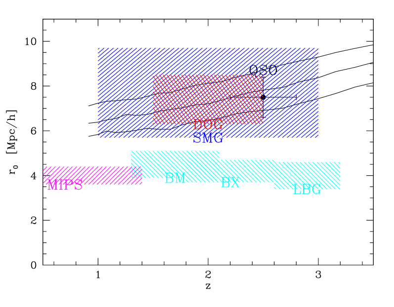
In Fig. 17 we compared the clustering of our quasar sample to that of other well-studied objects at . The quasar clustering amplitude is similar to that of submillimetre galaxies, suggesting they live in similar mass halos, and stronger than the typical star forming population. This is consistent with an evolutionary picture in which a merger triggers a massive starburst that creates a submillimetre galaxy and which is then quenched by the formation of a bright quasar (e.g. Alexander & Hickox, 2012). The descendants of our quasar hosts will have comparable clustering amplitudes to the quasars themselves, indicating that they will likely evolve into massive, luminous early-type galaxies at low redshift.
To better understand the possible fate of quasar host halos we employ another high-resolution N-body simulation which allows us to track halos and subhalos down to (for details see White, Cohn & Smit, 2010). We select all halos at which are central subhalos of halos which lie within an octave (i.e. factor of 2) in mass centered on ( particles). Essentially all of these halos are the most massive in their local environment. One quarter of the hosts fall into a large halo (becoming a satellite) and then lose more than 99.9 per cent of their mass (falling below the resolution limit of the simulation) without merging with the central galaxy or another satellite subhalo. To the extent that this process is well resolved, the stars in any galaxies hosted by these subhalos would likely contribute to an intra-halo light component, while the black holes would form a freely floating component or be associated with highly stripped satellites. Of the remaining 75 per cent of the subhalos, three quarters are the most massive progenitor in all their subsequent mergers and remain central galaxies to . The remaining quarter become satellites which survive to inside more massive halos. As a whole the population inhabits halos over a broad range of masses () peaking at . Halos of this group scale host galaxies of a few today, a population dominated by elliptical galaxies. This wide diversity of outcomes is reminiscent of the varied fates of star-forming galaxies (e.g. Conroy et al., 2008). As constraints on the stellar masses of galaxies within halos become tighter, comparison of the stellar masses of quasar hosts with that of their descendants will put constraints on the star-formation history of these objects.
The evolution of clustering with time can place strong constraints on how episodic quasar activity can be. As emphasized by Croom et al. (2005), if the typical host of quasars does not evolve significantly with redshift then quasars cannot be repeated bursts of the same black hole because such black holes would live in halos which grow in mass as the Universe evolves. However the quantitative strength of this statement, and the allowed fraction of objects which could burst more than once, is difficult to assess. One issue is the size of the observational errors, the other is that higher redshift samples typically probe more massive black holes than lower redshift samples (as emphasized e.g. by Hopkins et al., 2007b).
For example, the highest redshift clustering measurement comes from Shen et al. (2007), at . Their result is consistent with host halos of . Such hosts would grow in mass by a factor of approximately 4 between and 2.4. Similarly, the progenitors of our , halos are approximately 4 times less massive at . This suggests on average an order of magnitude mismatch in halo masses, but with a large error. Assuming no evolution in Eddington ratio between and the quasars in the Shen et al. (2007) sample are a factor of about 5 brighter than the BOSS quasars. If the power-law index of the relation is close to unity there is little tension from clustering777The dramatic decrease in quasar numbers to higher redshift does impose constraints. in assuming quasars episodically burst.
The time span between and in our adopted cosmology is Gyr. The Universe is another Gyr older at . Taking at from Ross et al. (2009) and converting it to a host halo mass we obtain . The descendants of our , halos are approximately twice as massive at , again leading to little tension in a model with episodic outbursts.
We can see the issues most clearly in Fig. 12. If halos moved with the same large-scale velocities as the dark matter and never merged the decrease of their bias would approximately cancel the increased clustering of the matter (Fry 1996; see Fig. 1 of White, et al. 2007). For a highly biased sample such passive evolution corresponds to almost constant clustering strength, for slightly less-biased objects the clustering strength grows slowly with time. This result is shown as the dashed line in Fig. 12, corresponding to objects with . Merging of halos and including a finite range of halo masses alters the details of this evolution, but keeps the sense unaltered. By contrast, halos of a fixed mass predict a clustering strength which drops slowly with time – shown as the dotted line in Fig. 12 for halos of . Again, a more realistic scenario with a finite range of halo masses has the same sense of the evolution. The current data are not in strong conflict with either scenario. If a random fraction of quasars repeats at later epochs while new quasars always appear in halos of a fixed mass, the measured clustering resembles a sample with bias . The measured values of are consistent with being roughly constant over . For this reason it is difficult to put a strong upper limit on the fraction of quasars that turn on more than once or the maximum number of times a given quasar can burst.
5 Conclusions
We have performed real- and redshift-space clustering measurements of a uniform subsample of quasars observed by the Baryon Oscillation Spectroscopic Survey (BOSS). These quasars lie in the redshift range where there has previously been a gap in coverage due to the fact that the quasar and stellar loci cross and the difficulty in targeting quasars in large numbers to faint fluxes. We detect clustering at high significance in both real- and redshift-space for the entire sample and subsamples split by redshift and luminosity (see Table 3). We do not detect a luminosity or redshift dependence of the clustering strength, although our sensitivity to this dependence is weak due to the limited dynamic range in both variables in our sample.
The two-point correlation functions are consistent with power-laws over the range of scales measured, with an underlying real-space clustering of the form . The correlation length, , does not appear to evolve strongly over the redshift range to . This result is consistent with passive evolution of a highly biased population, although this interpretation is by no means unique. Our results are consistent with quasars living in halos of typical mass at , in line with expectations from earlier surveys. The measured bias and space density of quasars can be used to infer their duty cycle (Cole & Kaiser, 1989). For our best-fit models the duty cycle peaks at one per cent, implying an activity time of years. This time is comparable to the activity times inferred for quasars at lower redshift, although the Hubble time at is shorter than at lower and hence the active fraction is larger.
The typical host halo mass is similar to the inferred hosts of submillimetre galaxies and is more massive than the inferred hosts of typical star-forming galaxies at the same redshift. This interpretation is in turn consistent with an evolutionary picture in which a massive starburst creates a submillimetre galaxy and is quenched by the formation of a bright quasar. While the typical descendant of the halos that host BOSS quasars is likely to host a luminous, elliptical galaxy at the present time, we find a wide diversity in descendants in N-body simulations.
Using abundance matching to infer the properties of quasar host galaxies we find evidence for evolution in the relation in the sense that black holes must be more massive at fixed galaxy mass at than at . We find that the predictions for how quasar activity and clustering (bias) depend on luminosity differ depending on whether we take as our fundamental relationship a black hole-halo correlation or a black hole-galaxy correlation. This is because the efficiency of galaxy formation is strongly (halo) mass dependent for the halos of interest at these redshifts, leading to strong curvature in the relation. In either scenario a modest scatter between halo or galaxy mass and observed quasar luminosity (arising, for example, from a combination of scatters in the black-hole bulge, bulge galaxy and galaxy halo correlations and the Eddington ratio) leads to a shallow dependence of clustering on quasar luminosity, as observed.
Future surveys of quasars which probe different regions of the luminosity–redshift plane will inform models of quasar formation and evolution. In this regard BOSS continues to measure quasar redshifts, and we expect the number of quasars in the luminosity and redshift range discussed here will be more than doubled by the end of the survey. It may be possible to incorporate the additional, BONUS quasars through cross-correlation or to cross-correlate spectroscopic and photometric quasar samples to better allow us to break the sample by luminosity, spectral or radio properties. In addition BOSS is measuring redshifts for a large sample of quasars, and analysis of those data will be crucial in understanding the early phases of quasar growth.
Funding for SDSS-III has been provided by the Alfred P. Sloan Foundation, the Participating Institutions, the National Science Foundation, and the U.S. Department of Energy Office of Science. The SDSS-III web site is http://www.sdss3.org/.
SDSS-III is managed by the Astrophysical Research Consortium for the Participating Institutions of the SDSS-III Collaboration including the University of Arizona, the Brazilian Participation Group, Brookhaven National Laboratory, University of Cambridge, Carnegie Mellon University, University of Florida, the French Participation Group, the German Participation Group, Harvard University, the Instituto de Astrofisica de Canarias, the Michigan State/Notre Dame/JINA Participation Group, Johns Hopkins University, Lawrence Berkeley National Laboratory, Max Planck Institute for Astrophysics, Max Planck Institute for Extraterrestrial Physics, New Mexico State University, New York University, Ohio State University, Pennsylvania State University, University of Portsmouth, Princeton University, the Spanish Participation Group, University of Tokyo, University of Utah, Vanderbilt University, University of Virginia, University of Washington, and Yale University.
The analysis made use of the computing resources of the National Energy Research Scientific Computing Center, the Shared Research Computing Services Pilot of the University of California and the Laboratory Research Computing project at Lawrence Berkeley National Laboratory.
M.W. was supported by the NSF and NASA. A.D.M. is a research fellow of the Alexander von Humboldt Foundation of Germany. JM is supported by Spanish grants AYA2009-09745 and PR2011-0431. JB was partially supported by a NASA Hubble Fellowship (HST-HF-51285.01)
Appendix A Redshift errors
At the signal-to-noise ratio and redshift at which BOSS is working it is difficult to obtain precise redshifts for quasars. Emission lines, such as Mgii which are good redshift indicators and which can be used at lower redshift, have redshifted into a relatively noisy part of the spectrum or off of the device altogether. One hour integrations on a m telescope make it difficult to measure redshifts for quasars with weak lines.
The BOSS pipeline measures quasar redshifts by fitting their spectra to a set of PCA templates (Aihara et al., 2011) plus a cubic polynomial to allow for changes in continuum slope. The reduced vs. redshift is mapped in steps of from to and the template fit with the best reduced is selected as the redshift. In addition redshifts are computed by fitting any lines in two groups (forbidden and allowed). A comparison of redshifts determined from different lines (Hennawi et al., 2006b; Shen et al., 2007), and visual inspections, suggests the automatic redshifts are good to . At this corresponds to an error in the line-of-sight distance of roughly Mpc (comoving), which is significant compared to the correlation length of quasar clustering. We are attempting to improve our quasar redshift determination, but for now we simply account for the residual line-of-sight smearing induced by redshift errors in our fitting.

In the limit the redshift-space halo correlation function is approximately isotropic and a power-law. If the redshift errors on quasars are uncorrelated and Gaussian distributed with fixed amplitude the observed correlation function is
| (16) |
where . The integral, , divided by the input power-law is what we refer to in the main text as .
Fig. 18 compares this model, with a power-law correlation function of slope 1.8, to halos from N-body simulations with applied Gaussian line-of-sight velocity errors. As expected, the agreement is excellent. In this test the redshift errors were all drawn from a Gaussian of the same dispersion. In the observational sample we might reasonably expect the errors to depend on the properties of each quasar. In this situation we should interpret as a pair-weighted, “effective”, redshift error. The above tests, plus the clustering measurements themselves, are consistent with a per quasar redshift error corresponding to Mpc, and we use that as our fiducial value throughout.
Appendix B Quasar model
Models of the quasar phenomenon come in several basic flavors, but are in fact all quite similar. The majority of models assume that quasar activity occurs due to the major merger of two gas-rich galaxies, since this scenario provides the rapid and violent event needed to funnel fuel to the center of the galaxy (e.g. via the bars-within-bars instability Shlosman et al., 1989) and feed the central engine while at the same time giving a connection between black hole fueling and the growth of a spheroidal stellar component. If black hole growth is feedback limited, it is only a rapidly growing potential well that can host a rapidly accreting hole. A notable exception is the models of Ciotti & Ostriker (1997, 2001) which postulate the fuel is funneled to the center by thermal instabilities, which provide the rapid growth of the spheroidal component necessary for black hole growth. As we shall see, both sets of models can predict very similar halo occupancy.
Some models implement the physics directly in numerical simulations which attempt to track the hydrodynamics of the gas, with subgrid models for quasar and star formation and the associated feedback (Sijacki et al., 2007; Hopkins et al., 2008; De Graf et al., 2011). Other models work at the level of dark matter halos, but follow the same physics – in simplified form – semi-analytically (Cattaneo, Haehnelt & Rees, 1999; Kauffmann & Haehnelt, 2000, 2002; Volonteri, Haardt & Madau, 2003; Bromley, Somerville & Fabian, 2004; Granato et al., 2004; Croton et al., 2006; Monaco, Fontanot & Taffoni, 2007; Malbon et al., 2007; Bonoli et al., 2009; Fanidakis et al., 2012). Even more idealized are models which are built upon dark matter halos but use scaling relations or convenient functional forms to relate the quasar properties to those of their host halos (Efstathiou & Rees, 1988; Carlberg, 1990; Wyithe & Loeb, 2002, 2003; Haiman, Ciotti & Ostriker, 2004; Marulli et al., 2006; Lidz et al., 2006; Croton, 2009; Shen, 2009; Booth & Schaye, 2010). A final level of abstraction is to simply provide a stochastic recipe for populating dark matter halos with quasars which is tuned to reproduce the observations as best as possible while not attempting to follow the underlying physics (Porciani, Magliocchetti & Norberg, 2004; White, Martini & Cohn, 2008; Padmanabhan et al., 2009; Shankar, Weinberg & Shen, 2010; Volonteri & Stark, 2011; Krumpe et al., 2012; Kirkpatrick et al., 2012).
The modeling is simplified by several facts. Quasars are rare, their activity times are short and the fraction of binary quasars is small (Hennawi et al., 2006a; Myers et al., 2007b). The hydrodynamic and semi-analytic models tend to reproduce the observed, relation between black hole mass and halo, which is used as input to the scaling models. The models agree on the level of scatter in the relation (roughly a factor of two) and in broad brush on the evolution in the amplitude and slope of this relation with redshift. Some models invoke quasar feedback limited accretion explicitly while others achieve the same scaling relations without such a limit—e.g., by coupling the mechanisms by which bulges and black holes grow. At these masses and redshifts the satellite galaxy fraction is tiny, so the halo to stellar mass relation is set by abundance matching and any model which reproduces the galaxy stellar mass function will reproduce this relation. At high redshift bright quasars radiate near Eddington, so the models predict similar halo occupancies.
The probability that a halo will undergo a major merger in a short redshift interval is only weakly dependent on the mass of the halo (Lacey & Cole, 1993; Percival et al., 2003; Cohn & White, 2005; Wetzel, Cohn & White, 2009; Fakhouri & Ma, 2009; Hopkins et al., 2010), i.e. the mass function of such halos is almost proportional to the mass function of the parent population. Similarly the clustering properties of recently merged halos are similar to a random sample of the population with the same mass distribution (Percival et al., 2003; Wetzel, Cohn & White, 2009). Thus in any interval, , the fraction of halos of mass which undergo a quasar event is almost independent of and and can be regarded as a random selection. This makes it difficult to infer that quasars arise from mergers simply from their large-scale clustering, but also implies that for the purposes of modeling the 1- and 2-point functions of the quasar population it is sufficient to specify the halo occupation of the parent population (more complex models may be needed if correlations between quasars and properties of e.g. galaxies were required).
To determine whether a quasar candidate makes it into any sample it is necessary to relate the observed luminosity to the peak luminosity which is determined by . This is done either by specifying a light curve (e.g. a power-law, a power-law with a varying slope or an exponential) or directly using the fact that the triggering rate is understood. For constant triggering rate a light curve implies , so a wide range of maps to a narrow range in index. For the high luminosity thresholds we only see objects very near their peak brightness. Taking into account the factor scatter in at fixed bulge mass, we expect to be roughly lognormal with a similar width (it can be slightly broader due to variation in the Eddington ratio at peak). As we probe lower luminosities we are more likely to see older, more massive black holes leading to a low tail in and more lower-Eddington-ratio objects (Lidz et al., 2006; Shen, 2009; Cao, 2010). Unless we cut off the probability that a halo hosts a quasar at low and high halo mass, we will overproduce low and high sources (Lidz et al., 2006; Croton, 2009; Shen, 2009). In the physical models these limits occur due to lack of fuel in low mass halos and the inability of gas to cool in high-mass halos (e.g. Cattaneo, Haehnelt & Rees, 1999). As discussed in §4.2, models which match the relation for galaxies tend to roughly match the required quasar suppression.
We are interested in the probability that a given halo hosts a quasar in our sample, e.g. . From the arguments above we expect this relation to be an approximately lognormal function which is asymmetric towards high at low . It is quite difficult to put constraints on the detailed form of this function using luminosity function and clustering measurements.
We argued above that the steepness of the halo mass function and the high bias of quasars implies that the quasar satellite fraction is small. The luminosity function thus provides a constraint on the duty cycle. (This extra degree of freedom reduces the ability of large-scale structure measurements to constrain the halo occupancy, compared to modeling galaxies.) The steeply falling mass function also implies that the number of quasars hosted in very massive halos is small regardless of the occupancy statistics of such halos. On scales larger than the virial radius of the typical quasar host halo (i.e. kpc) the 2-point function is dominated by pairs of quasars in different halos, and thus primarily measures the quasar-weighted halo bias which allows us to infer the mean, quasar-weighted halo mass. This result remains true for cross-correlation studies too, provided we work on scales larger than the virial radius of the quasar hosts. On smaller scales the amplitude and slope of the correlation function allow us to measure a combination of the satellite fraction of quasars and the low mass cutoff.
References
- Abazajian et al. (2004) Abazajian K., Adelman-McCarthy J.K., Agüeros M.A., et al., 2004, AJ, 128, 502
- Adelberger et al. (2005) Adelberger K.L., Steidel C.C., Pettini M., Shapley A.E., Reddy N.A., Erb D.K., 2005, ApJ, 619, 697
- Adelman-McCarthy et al. (2007) Adelman-McCarthy J., et al., 2007, ApJS, 172, 634
- Aihara et al. (2011) Aihara H., et al., 2011, ApJS, 193, 29 [erratum, ApJS, 195, 26]
- Alexander & Hickox (2012) Alexander D.M., Hickox R.C., 2012, to appear in New Astronomy Reviews [arxiv:1112.1949]
- da Angela et al. (2008) da Angela J., et al., 2008, MNRAS, 383, 565
- Anderson et al. (2012) Anderson L., et al., 2012, submitted to MNRAS [arxiv:1203.6594]
- Behroozi, Conroy & Wechsler (2010) Behroozi P.S., Conroy C., Wechsler R.H., 2010, ApJ, 717, 379
- Blanton et al. (2003) Blanton M.R., Lin H., Lupton R.H., Maley F.M., Young N., Zehavi I., Loveday J., 2003, AJ, 125, 2276
- Bonoli et al. (2009) Bonoli S., Marulli F., Springel V., White S.D.M., Branchini E., Moscardini L., 2009, MNRAS, 396, 423
- Booth & Schaye (2010) Booth C.M., Schaye J., 2010, MNRAS, 405, L1
- Bovy et al. (2009) Bovy J., Hogg D.W., Roweis S.T., 2009, AOAS, 5, 1657 [arXiv:0905.2979]
- Bovy et al. (2011) Bovy J., et al., 2011, ApJ, 729, 141
- Bovy et al. (2012) Bovy J., et al., 2012, ApJ, 749, 41 [arXiv:1105.3975 ]
- Brodwin et al. (2008) Brodwin M., Dey A., Brown M.J.I., Pope A., Armus L., Bussmann S., Desai V., Jannuzi B.T., le Floch E., 2008, ApJ, 687, L65
- Bromley, Somerville & Fabian (2004) Bromley J.M., Somerville R.S., Fabian A.C., 2004, MNRAS, 350, 456
- Budavári et al. (2001) Budavári T., et al., 2001, AJ, 122, 1163
- Cao (2010) Cao X., 2010, ApJ, 725, 388
- Carlberg (1990) Carlberg R.G., 1990, ApJ, 350, 505
- Cattaneo, Haehnelt & Rees (1999) Cattaneo A., Haehnelt M.G., Rees M.J., 1999, MNRAS, 308, 77
- Ciotti & Ostriker (1997) Ciotti L., Ostriker J.P., 1997, ApJ, 487, 105
- Ciotti & Ostriker (2001) Ciotti L., Ostriker J.P., 2001, ApJ, 551, 131
- Cohn & White (2005) Cohn J.D., White M., 2005, Astroparticle Physics, 24, 316
- Cole & Kaiser (1989) Cole S., Kaiser N., 1989, MNRAS, 237, 1127
- Conroy et al. (2008) Conroy, C., Shapley A., Tinker J.L., Santos M.R., Lemson G., 2008, ApJ, 679, 1192
- Croom et al. (2004) Croom S.M., et al., 2004, MNRAS, 349, 1397
- Croom et al. (2005) Croom S.M., et al., 2005, MNRAS, 356, 415
- Croom et al. (2009) Croom S.M., et al., 2009, MNRAS, 392, 19
- Croton et al. (2006) Croton D.J., et al., 2006, MNRAS, 365, 11
- Croton (2009) Croton D.J., 2009, MNRAS, 394, 1109
- Davis et al. (1985) Davis M., Efstathiou G., Frenk C.S., White S.D.M., 1985, ApJ, 292, 371
- Decarli et al. (2010) Decarli R., Falomo R., Treves A., Labita M., Kotilainen J.K., Scarpa R., 2010, MNRAS, 402, 2453
- Doi et al. (2010) Doi M., et al., 2010, AJ, 139, 1628
- Efron & Gong (1983) Efron, B., Gong, G., 1983, American Statistician, 37, 36
- Efstathiou & Rees (1988) Efstathiou G., Rees M.J., 1988, MNRAS 230, 5
- Eisenstein et al. (2011) Eisenstein D.J., et al., 2011, AJ 142, 72
- Fakhouri & Ma (2009) Fakhouri O., Ma C.-P., 2009, MNRAS, 394, 1825
- Fan (1999) Fan X., 1999, AJ, 117, 2528
- Fanidakis et al. (2012) Fanidakis N., Baugh C.M., Benson A.J., Bower R.G., Cole S., Done C., Frenk C.S., Hickox R.C., Lacey C., del P. Lagos C., 2012, MNRAS, 419, 2797
- Ferrarese (2002) Ferrarese, L. 2002, ApJ, 578, 90
- Fine et al. (2006) Fine S., et al., 2006, MNRAS, 373, 613
- Fry (1996) Fry J.N., 1996, ApJ, 461, L65
- Fukugita et al. (1996) Fukugita, M., Ichikawa, T., Gunn, J.E., Doi, M., Shimasaku, K., Schneider D.P., 1996, AJ, 111, 1748
- Gilli et al. (2007) Gilli R., Daddi E., Chary R., Dickinson M., Elbaz D., Giavalisco M., Kitzbichler M., Stern D., Vanzella E., 2007, A&A, 475, 83
- Gorski et al. (2005) Gorski K.M., Hivon E., Banday A.J., Wandelt B.D., Hansen F.K., Reinecke M., Bartelmann M., 2005, ApJ, 622, 759 [astro-ph/0409513]
- De Graf et al. (2011) De Graf C., Di Matteo T., Khandai N., Croft R., Lopez J., Springel V., 2011, preprint [arxiv:1107.1254]
- Graham (2012) Graham A., 2012, ApJ, 746, 113 [arxiv:1202.1878]
- Granato et al. (2004) Granato G.L., de Zotti G., Silva L., Bressan A., Luigi D., 2004, ApJ, 600, 580
- Gunn et al. (1998) Gunn, J.E., et al. 1998, AJ, 116, 3040
- Gunn et al. (2006) Gunn, J.E., et al. 2006, AJ, 131, 2332
- Haiman & Hui (2001) Haiman Z., Hui L., 2001, ApJ, 547, 27
- Haiman, Ciotti & Ostriker (2004) Haiman Z., Ciotti L., Ostriker J.P., 2004, ApJ, 606, 763
- Haiman & Loeb (1998) Haiman Z., Loeb A., 1998, ApJ, 503, 505
- Haring & Rix (2004) Haring N., Rix H., 2004, ApJ, 604, L89
- Hartwick & Schade (1990) Hartwick F.D.A., Schade D., 1990, ARA&A, 28, 437
- Hawkins et al. (2003) Hawkins E., et al., 2003, MNRAS, 346, 78
- Hennawi et al. (2006a) Hennawi J.F., et al., 2006a, AJ, 131, 1
- Hennawi et al. (2006b) Hennawi J.F., et al., 2006b, ApJ, 651, 61
- Hewett & Wild (2010) Hewett P.C., Wild V., 2010, MNRAS, 405, 2302
- Hickox et al. (2011) Hickox R., et al., 2011, ApJ, 731, 117
- Hickox et al. (2012) Hickox R., et al., 2012, MNRAS, 421, 284 [arxiv:1112.0321]
- Hopkins et al. (2006) Hopkins P.F., Somerville R.S., Hernquist L., Cox T.J., Robertson B., Li Y., 2006, ApJ, 652, 864
- Hopkins et al. (2007a) Hopkins P., Hernquist L., Cox T.J., Robertson B., Krause E., 2007a, ApJ, 669, 45.
- Hopkins et al. (2007b) Hopkins P., Lidz A., Hernquist L., Coil A.L., Myers A.D., Cos T.J., Spergel D.N., 2007b, ApJ, 662, 110
- Hopkins et al. (2008) Hopkins P.F., Hernquist L., Cox T.J., Keres D., 2008, ApJS, 175, 356
- Hopkins et al. (2010) Hopkins P., et al., 2010, ApJ, 724, 915
- Kaiser (1987) Kaiser N., 1987, MNRAS, 227, 1
- Kauffmann & Haehnelt (2000) Kauffmann G., Haehnelt M., 2000, MNRAS, 311, 576
- Kauffmann & Haehnelt (2002) Kauffmann G., Haehnelt M., 2002, MNRAS, 332, 529
- Kirkpatrick et al. (2012) Kirkpatrick J., et al., 2012, in preparation.
- Kormendy & Richstone (1995) Kormendy J., Richstone D., 1995, ARA&A, 33, 581
- Krumpe et al. (2012) Krumpe M., Miyaji T., Coil A.L., Aceves H., 2012, ApJ, 746, 1
- Krumpe, Miyaji & Coil (2010) Krumpe M., Miyaji T., Coil A.L., 2010, ApJ, 713, 558
- Lacey & Cole (1993) Lacey C., Cole S., 1993, MNRAS, 262, 627
- Landy & Szalay (1993) Landy S.D., Szalay A.S., 1993, ApJ, 412, 64
- Li et al. (2006) Li, C., Kauffmann, G., Jing, Y. P., White, S. D. M., Börner, G., Cheng, F. Z., 2006, MNRAS, 368, 21
- Lidz et al. (2006) Lidz A., Hopkins P.F., Cox T.J., Hernquist L., Robertson B., 2006, ApJ, 641, 41.
- Lupton et al. (2001) Lupton, R., Gunn, J. E., Ivezic, Z., Knapp, G. R., Kent, S. 2001, in ASP Conf. Ser. 238, Astronomical Data Analysis Software and Systems X, ed. F. R. Harnden, Jr., F. A. Primini, H. E. Payne (San Francisco, CA: ASP), 269
- Lynden-Bell (1969) Lynden-Bell D., 1969, Nature, 223, 690
- Malbon et al. (2007) Malbon R.K., Baugh C.M., Frenk C.S., Lacey C.G., 2007, MNRAS, 382, 1394
- Martini & Weinberg (2001) Martini P., Weinberg D.H., 2001, ApJ, 547, 12
- Marulli et al. (2006) Marulli F., Crociani D., Volonteri M., Branchini E., Moscardini L., 2006, MNRAS, 368, 1269
- Matarrese et al. (1997) Matarrese S., Coles P., Lucchin F., Moscardini L., 1997, MNRAS, 286, 115
- Di Matteo et al. (2012) Di Matteo T., Khandai N., DeGraf C., Feng Y., Croft R.A.C., Lopez J., Springel V., 2012, ApJ, 745, L29
- Merloni et al. (2010) Merloni A., et al., 2010, ApJ, 708, 137
- Monaco, Fontanot & Taffoni (2007) Monaco P., Fontanot F., Taffoni G., 2007, MNRAS, 375, 1189
- Moster et al. (2010) Moster B.P., et al., 2010, ApJ, 710, 903
- Myers et al. (2006) Myers A.D., et al., 2006, ApJ, 638, 622
- Myers et al. (2007a) Myers A.D., Brunner R.J., Nichol R.C., Richards G.T., Schneider D.P., Bahcall N.A., 2007a, ApJ, 658, 85
- Myers et al. (2007b) Myers A.D., Brunner R.J., Nichol R.C., Richards G.T., Schneider D.P., Bahcall N.A., 2007b, ApJ, 658, 99
- Myers, White & Ball (2009) Myers A.D., White M., Ball N., 2009, MNRAS, 399, 2279
- Nandra et al. (2007) Nandra, K., et al., 2007, ApJL, 660, L11
- Natarajan (2012) Natarajan P., 2012, in “Proceedings of the XVth Congress of Philosophy & Foundations of Science”, to be published by the American Institute of Physics [arxiv:1105.4902]
- Padmanabhan et al. (2008) Padmanabhan, N., et al. 2008, ApJ, 674, 1217
- Padmanabhan et al. (2009) Padmanabhan N., White M., Norberg P., Porciani C., 2009, MNRAS, 397, 1862
- Peng et al. (2006) Peng C.Y., Impey C.D., Rix H-W., Falco E.E., Keeton C., Kochanek C.S., Lehar J., McLeod B.A., 2006, NewAR, 50, 689
- Percival et al. (2003) Percival W.J., Scott D., Peacock J.A., Dunlop J.S., 2003, MNRAS, 338, L31
- Pier et al. (2003) Pier J.R., Munn, J. A., Hindsley, R. B., Hennessy, G. S., Kent, S. M., Lupton, R. H., Ivezic, Z., 2003, AJ, 125, 1559
- Porciani, Magliocchetti & Norberg (2004) Porciani C., Magliocchetti M., Norberg P., 2004, MNRAS, 355, 1010
- Porciani & Norberg (2006) Porciani C., Norberg P., 2006, MNRAS, 371, 1824
- Reid et al. (2012) Reid B.A., Samushia L., White M., Percival W.J., et al., 2012, submitted to MNRAS [arxiv:1203.6641]
- Richards et al. (2001) Richards G.T., et al., 2001a, AJ, 121, 2308
- Richards et al. (2001) Richards G.T., et al., 2001b, AJ, 122, 1151
- Richards et al. (2002a) Richards, G.T., et al., 2002a, AJ, 123, 2945
- Richards et al. (2002b) Richards, G.T., et al., 2002b, AJ, 124, 1
- Richards et al. (2006) Richards G.T., et al., 2006, AJ, 131, 2766
- Richards et al. (2009) Richards G.T., et al., 2009, ApJS, 180, 67
- Richards et al. (2011) Richards, G.T., et al., 2011, AJ, 141, 167
- Ross et al. (2007) Ross N.P., et al., 2007, MNRAS, 381, 573
- Ross et al. (2009) Ross N.P., et al., 2009, ApJ, 697, 1634
- Ross et al. (2012) Ross N.P., et al., 2012, ApJS, 199, 3 [arxiv:1105.0606]
- Salpeter (1964) Salpeter, E.E., 1964, ApJ, 140, 796
- Schneider et al. (2010) Schneider D.P., et al., 2010, AJ, 139, 2360
- Shankar (2009) Shankar F., 2009, New AR, 53, 57
- Shankar, Weinberg & Shen (2010) Shankar F., Weinberg D.H., Shen Y., 2010, MNRAS, 406, 1959
- Shanks et al. (2011) Shanks, T., Croom, S.M., Fine, S., Ross, N.P., Sawangwit, U., 2011, MNRAS, 416, 650
- Shen et al. (2007) Shen Y., et al., 2007, AJ, 133, 2222
- Shen (2009) Shen Y., 2009, ApJ, 704, 89
- Shen et al. (2009) Shen Y., et al., 2009, ApJ, 697, 1656
- Shlosman et al. (1989) Shlosman I., Frank J., Begelman M.C., 1989, Nature, 338, 45
- Sijacki et al. (2007) Sijacki D., Springel V., Di Matteo T., Hernquist L., 2007, MNRAS 380, 877
- Silk & Rees (1998) Silk J., Rees M.J., 1998, A&A, 331, L1
- Silverman et al. (2008) Silverman, J. D., et al., 2008, ApJ, 679, 118
- Smith et al. (2002) Smith J.A., et al., 2002, AJ, 123, 2121
- Smith et al. (2003) Smith R.E., Peacock J.A., Jenkins A., White S.D.M., Frenk C.S., Pearce F.R., Thomas P.A., Efstathiou G., Couchman H.M.P., 2003, MNRAS, 341, 1311
- Springel et al. (2005) Springel V., Di Matteo T., Hernquist L., 2005, MNRAS, 361, 776
- Swanson et al. (2008) Swanson M.E.C., Tegmark M., Hamilton A.J.S., Hill J.C., 2008, MNRAS, 387, 1391
- Tegmark et al. (2004) Tegmark M., et al., 2004, ApJ, 606, 702
- Tremaine et al. (2002) Tremaine S., et al., 2002, MNRAS, 574, 740
- Vanden Berk et al. (2001) Vanden Berk D.E., et al., 2001, AJ, 122, 549
- Volonteri, Haardt & Madau (2003) Volonteri M., Haardt F., Madau P., 2003, ApJ, 582, 559
- Volonteri & Stark (2011) Volonteri M., Stark D.P., 2011, MNRAS, 417, 2085
- Weedman (1986) Weedman D., 1986, “Quasar Astronomy”, Cambridge University Press, Cambridge.
- Weinstein et al. (2004) Weinstein M.A., et al., 2004, ApJS, 155, 243
- Wetzel, Cohn & White (2009) Wetzel A., Cohn J.D., White M., 2009, MNRAS, 394, 2182
- White (2002) White M., 2002, ApJS, 579, 16
- White, et al. (2007) White M., Zheng Z., Brown M.J.I., Dey A., Jannuzi B.T., 2007, ApJ, 655, L69
- White, Martini & Cohn (2008) White M., Martini P., Cohn J.D., 2008, MNRAS, 390, 1179
- White et al. (2011) White M., et al., 2011, ApJ, 728, 126
- White, Cohn & Smit (2010) White M., Cohn J.D., Smit R., 2010, MNRAS, 408, 1818
- Wyithe & Loeb (2002) Wyithe J.S.B., Loeb A., 2002, ApJ, 581, 886
- Wyithe & Loeb (2003) Wyithe J.S.B., Loeb A., 2003, ApJ, 595, 614
- York et al. (2000) York, D. G., et al. 2000, AJ, 120, 1579