A fast high-order method to calculate wakefield forces in an electron beam

Abstract

In this paper we report on a high-order fast method to numerically calculate wakefield forces in an electron beam given a wake function model. This method is based on a Newton-Cotes quadrature rule for integral approximation and an FFT method for discrete summation that results in an $O(Nlog(N))$ computational cost, where $N$ is the number of grid points. Using the Simpson quadrature rule with an accuracy of $O(h^{4})$, where $h$ is the grid size, we present numerical calculation of the wakefields from a resonator wake function model and from a one-dimensional coherent synchrotron radiation (CSR) wake model. Besides the fast speed and high numerical accuracy, the calculation using the direct line density instead of the first derivative of the line density avoids numerical filtering of the electron density function for computing the CSR wakefield force.

I Introduction

The wakefield forces from the interaction of electrons with external materials and from the interactions of electrons inside the beam through radiation have significant effects on the electron beam quality for next generation light sources. Those wakefields can cause the loss of beam energy, increase the beam energy spread, increase beam emittance through the magnetic bunch compressor, and drive microbunching instability through the linac. Including the wakefield effects in a beam dynamics tracking code is crucial for designing a beam delivery system for next generation light sources and has been included in a number of tracking codes qiang0 ; elegant ; lietrack ; qiang00 .

The numerical calculation of the wakefield forces on electrons involves calculating a convolution between the wake function and the charge density of the beam. The direct numerical calculation of the convolution for the wakefield has a computational cost scaling as $O(N^{2})$, where $N$ is the number of grid points in the computational domain. Fortunately, such a discretized convolution summation on a uniform grid can be calculated using a cyclic summation on a doubled computational domain using an FFT based method hockney ; nr ; qiang3 ; ryne1 . This reduces the computational cost from $O(N^{2})$ to $O(Nlog(N))$. In our previous study, we have developed a high-order FFT based method to numerically calculate the convolution with a smooth kernel qiang1 . In this paper, we extend the previous study by applying a high-order Simpson quadrature rule to the wakefield convolution with finite discontinuity of the kernel. We then apply this method to the calculation of the wakefields from an external resonator wake function (an approximation to the AC resistance wall wake function) and from a steady-state CSR wake function.

The organization of the paper is as follows: after a brief introduction, we present the computational method in Section 2, application examples to calculate the wakefield forces from an external resonator wake function and from a steady-state CSR wake function in Section 3, and final summary in Section 4.

II Computational Method

We consider the longitudinal wakefield on an electron at longitudinal location $z$ inside an electron beam can be written as

$$E(z) = \int_{-\infty}^{\infty}W(z-z^{\prime})\rho(z^{\prime})dz^{\prime}$$ (1)

where $W$ is the wake function from the interaction of electrons with external materials such as resistive wall wake or the interaction among electrons themselves such as the coherent synchrotron radiation (CSR) inside a bending magnet, and $\rho$ is the beam line density distribution. For the external wake function, the variable $z$ stands for $ct$, where $t$ is the time of flight difference with respect to the head of the beam, and $c$ is the speed of light in vacuum. For the CSR wake function, the variable $z$ stands for the longitudinal spatial position. The above convolution integral can be written as the summation of $M$ equal subinterval integrals:

$$E(z) = \sum_{i=1}^{M}\int_{z^{\prime}_{i}}^{z^{\prime}_{i+1}}W(z-z^{\prime})\rho(z^{\prime})dz^{\prime}$$ (2)

where $z^{\prime}_{i}=(i-1)(z/M),i=1,\cdots,M$. For the integral between $z^{\prime}_{i}$ and $z^{\prime}_{i+1}$, the closed Newton-Cotes formula of degree $k$ at $k+1$ equally spaced points can be written as

$$\int_{z^{\prime}_{i}}^{z^{\prime}_{i+1}}W(z-z^{\prime})\rho(z^{\prime})dz^{\prime} \approx \sum_{j=0}^{k}w_{j}W(z-z^{\prime}_{j})\rho(z^{\prime}_{j})$$ (3)

where $z^{\prime}_{j}=z^{\prime}_{i}+jdz$, $dz=z/(kM)$, and the weight $w_{j}$ is associated with integral of the $j_{th}$ Lagrange basis polynomial. For $k=1$, this is known as the trapezoidal quadrature rule; for $k=2$, this is the Simpson rule; for $k=3$, Simpson’s $3/8$ rule; for $k=4$, Boole’s rule, etc math ; math2 . Using the extended three-point Simpson rule on a uniform grid, the above convolution integral can be approximated as

$$E(z) = \bar{E}(z)+O(h^{4})$$ (4)

where $h$ is the grid size, and $\bar{E}(z)$ is the numerical approximation of the convolution integral. For a grid point $z_{i}$, if $i$ is an odd number, the Simpson quadrature rule yields

$$\bar{E}(z_{i}) = \frac{1}{3}h(f_{1}+4\sum_{j=1}^{(i-1)/2}f_{2j}+2\sum_{j=2}^{(i-1)/2}f_{2j-1}+f_{i})$$ (5)

if $i$ is an even number, it yields

$$\bar{E}(z_{i}) = \frac{1}{3}h(3f_{1}/2+5f_{2}/2+2\sum_{j=2}^{(i-2)/2}f_{2j}+4\sum_{j=2}^{i/2}f_{2j-1}+f_{i})$$ (6)

where the kernel function $f$ is given by

$$f(z,z^{\prime}) = W(z-z^{\prime})\rho(z^{\prime})$$ (7)

and $f_{j}(z_{i})=f(z_{i},z^{\prime}_{j})$ with $z^{\prime}_{j}=(j-1)h$. The above numerical summation can be rewritten as

$$\bar{E}(z_{i}) = \frac{1}{3}h\sum_{j=1}^{N}\bar{W}(z_{i}-z_{j})\bar{\rho}(z_{j})+\frac{1}{3}hW(0)\rho(z_{i})$$ (8)

with

$$\bar{\rho}(z_{j}) = \left\{\begin{array}[]{r@{\quad:\quad}l}{\rho}(z_{j})&j=1\\ 4{\rho}(z_{j})&j=2l\\ 2\rho(z_{j})&j=2l-1\end{array}\right.$$ (12)

for odd grid number $i$, and

$$\bar{\rho}(z_{j}) = \left\{\begin{array}[]{r@{\quad:\quad}l}3{\rho}(z_{j})/2&j=1\\ 5{\rho}(z_{j})/2&j=2\\ 2{\rho}(z_{j})&j=2l\\ 4\rho(z_{j})&j=2l-1\end{array}\right.$$ (17)

for even grid number $i$, and the modified wake function $\bar{W}$ is given by

$$\bar{W}(z) = \left\{\begin{array}[]{r@{\quad:\quad}l}{W}(z)&z>0\\ 0&z\leq 0\end{array}\right.$$ (20)

The direct calculation of the above summation requires $O(N)$ operations for a single point $z_{i}$, where $i=1,\cdots,N$. To obtain the convolution for all $N$ points on the grid, the total computational cost will be $O(N^{2})$. Fortunately, the above convolution summation can be replaced by a cyclic summation in the double-gridded computational domain:

$$\bar{E}_{c}(z_{i}) = \frac{1}{3}h\sum_{j=1}^{2N}\bar{W}_{c}(z_{i}-z_{j})\bar{\rho}_{c}(z_{j})$$ (21)

where $i=1,\cdots,2N$,  $j=1,\cdots,2N$ and

$$\bar{\rho}_{c}(z_{j}) = \left\{\begin{array}[]{r@{\quad:\quad}l}\bar{\rho}(z_{j})&1\leq j\leq N\\ 0&N<j\leq 2N\end{array}\right.$$ (24)

$$\bar{W}_{c}(z_{k}) = \left\{\begin{array}[]{r@{\quad:\quad}l}\bar{W}(z_{k})&1\leq k\leq N;\\ \bar{W}(-z_{2N+2-k})&N<k\leq 2N;\\ \end{array}\right.$$ (27)

where the new density function $\bar{\rho}_{c}(z)$ and the new wake function $\bar{W}_{c}(z)$ have the properties:

$$\bar{\rho}_{c}(z) = \bar{\rho}_{c}(z+2(L+h))$$ (28)

$$\bar{W}_{c}(z) = \bar{W}_{c}(z+2(L+h))$$ (29)

where $L=(N-1)h$. From above definition, one can show that the cyclic summation gives the same value as the convolution summation within the original domain, i.e.

$$\bar{E}(z_{i}) = \bar{E}_{c}(z_{i})\hskip 28.45274ptfor~{}\ i=1,\ N.$$ (30)

In the cyclic summation, the kernel is a discrete periodic function in the doubled computational domain. This cyclic summation can be calculated using the FFT method, i.e.

$$\bar{E}_{c}(z_{i}) = \it{InvFFT}(\bar{E}_{c}(\omega))$$ (31)

Here, $\it{InvFFT}$ denotes the inverse FFT of the function $\bar{E}_{c}(\omega)$ that is given by

$$\bar{E}_{c}(\omega) = \bar{W}_{c}(\omega)\ \bar{\rho}_{c}(\omega)$$ (32)

where $\bar{W}_{c}(\omega)$ and $\bar{\rho}_{c}(\omega)$ denote the forward FFT of the function $\bar{W}_{c}$ and the $\bar{\rho}_{c}$ respectively. The computational operations required to calculate cyclic summation using the above FFT method is of $O(Nlog(N)$.

III Application Examples

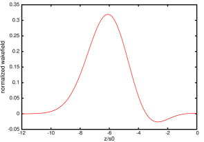
Figure 1: The wakefield force as a function of bunch length coordinate in an electron beam inside a Copper pipe with resonator wake function.

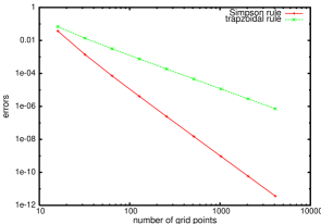
Figure 2: The errors at the center of the electron beam as a function grid points. The red line is from the Simpson quadrature rule and the green line is from the trapzoidal rule.

As an illustration, we use the above method to calculate the wakefields inside an electron beam from a resonator wake function and from the CSR wake function. The resonator wake function is given as bane

$$W(s) = \frac{4}{a^{2}}\exp(-(s/s_{0})/\Gamma)\cos((8/\Gamma)^{1/4}(s/s_{0}));\ for\ \ s\geq 0$$ (33)

where $s=z-z^{\prime}$ is the separation between the observation point and the source point, $s_{0}=(2a/(Z_{0}\sigma))^{1/3}$ is the characteristic length of the wake, $a$ is the radius of the pipe, $\sigma$ is the conductivity of the pipe material, $Z_{0}$ is the vacuum impedance, $\Gamma=c\tau/s_{0}$ is the normalized relaxation time, and $\tau$ is the relaxation time. This wake function provides a good approximation to the AC resistive wall wake function at large $\Gamma$ bane .

Figure 1 shows the normalized wakefield in an electron beam moving inside a Copper pipe ($\Gamma=1$) computed using the above algorithm. The beam has an rms bunch length of $1.5s_{0}$ and a Gaussian current distribution. The electron beam loses energy to the wall due to the resistance of the conducting pipe. To verify the accuracy of the above algorithm, Figure 2 shows the errors of the calculated wakefield at the center of the bunch as a function of the number of grid points. As a comparison, we also give the errors using the trapezoidal quadrature rule. As expected, the above Simpson rule method converges much faster than the trapezoidal rule based method. The accuracy of the Simpson rule calculated wakefield increases by more than an order of magnitude as the number of grid points doubles.

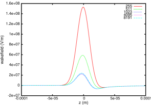
Figure 3: The CSR wakefield as a function of bunch length coordinate in an electron beam.

Another application example of above numerical method is to calculate the wakefield force from the one-dimensional steady state CSR wake. The one-dimensional CSR wake function is given as saldin

$$W(u(s)) = \frac{1}{4\pi\epsilon}\frac{\gamma^{4}}{R^{2}}\{\frac{u^{2}/4-1}{2(1+u^{2}/4)^{3}}+\frac{1/6-u^{2}/18-u^{4}/64}{(1+u^{2}/4)^{3}(1+u^{2}/12)^{2})}\}$$ (34)

and

$$u(s) = (\sqrt{64+144\bar{s}^{2}}+12\bar{s})^{1/3}-(\sqrt{64+144\bar{s}^{2}}-12\bar{s})^{1/3}$$ (35)

where $\bar{s}=\frac{s\gamma^{3}}{R}$ is the normalized longitudinal separation between the source point and the observation point, $R$ is the radius of the bending magnet, and $\gamma$ is the relativistic factor of the electron beam. The direct application of the above method with different number of grid points is shown in Fig. 3 for a $1$ nC Gaussian beam with $10$ micron rms bunch length at $100$ MeV. It is seen that a few thousand grid points are needed in order to obtain a numerically converged wakefield.

Figure 4: The steady-state CSR wake function as a function of separation between the observation point and the source point.

This large number of grid points is needed due to the sharp variation of the CSR wake function around $s=0$ as shown in Fig. 4. It is seen that outside this short range (about a few micron in this example) around zero, the CSR wake function is much smoother and can be approximated by an asymptotic function $s^{-4/3}$. Recently, an integrated Green function method with linear basis was proposed to treat the CSR wake function including the short range effect ryne . Here, we propose a modified Simpson rule method by separating the range of the original CSR wake function into two regions: one small region around the zero covering the short range CSR interaction, and the remainning region covering the long range interaction. The integral for the CSR wakefield can be written as:

$$E(z) = \int_{-\infty}^{z-\delta z}W(z-z^{\prime})\rho(z^{\prime})dz^{\prime}+\int_{z-\delta z}^{z}W(z-z^{\prime})\rho(z^{\prime})dz^{\prime}$$ (36)

where $\delta z$ is a small distance around the zero to separate the long-range CSR interaction from the short-range interaction. The first integral in the above equation can be calculated using a Simpson quadrature rule as shown in the previous section. Using the parameters in the above example with $\delta z=3.2\ um$ and the Simpson quadrature rule, we calculated the errors at the center of the bunch as a function of the number of grid points for the first integral in Eq. 36. The results are shown in Fig. 5.

Figure 5: The errors at the center of the bunch as a function of grid points for the first integral in Eq. 36 using the Simpson rule.

As expected, the error of the integral decreases by more than an order of magnitude as the number of the grid points doubles.

The second integral in the Eq. 36 will be calculated using an integrated Green’s function method with constant current density basis functions given the fact that the CSR wake function varies sharply while the line density changes slowly inside such a short-range interval. At each grid point $z_{i}$, the interval $[z_{i}-\delta z,z_{i}]$ is subdivided into $N_{int}$ number of sub-intervals with a length $h_{int}=\delta z/(N_{int}-1)$. This integral can now be rewritten as:

$$\int_{z_{i}-\delta z}^{z_{i}}W(z_{i}-z^{\prime})\rho(z^{\prime})dz^{\prime} = \int_{z_{1}}^{z_{1}+h_{int}/2}W(z_{i}-z^{\prime})\rho(z^{\prime})dz^{\prime}+\sum_{j=2}^{i-1}\int_{z_{j}-h_{int}/2}^{z_{j}+h_{int}/2}W(z_{i}-z^{\prime})\rho(z^{\prime})dz^{\prime}$$ (37)

$$+\int_{z_{i}-h_{int}/2}^{z_{i}}W(z_{i}-z^{\prime})\rho(z^{\prime})dz^{\prime}$$

where $z_{1}=z_{i}-\delta z$. Since the $\delta z$ is small (O($\mu m$)), only a small number of sub-intervals are needed. Assuming that the current density is constant within each sub-interval, the above integral can be approximated as:

$$\int_{z_{i}-\delta z}^{z_{i}}W(z_{i}-z^{\prime})\rho(z^{\prime})dz^{\prime} = \rho(z_{1})\int_{z_{1}}^{z_{1}+h_{int}/2}W(z_{i}-z^{\prime})dz^{\prime}+\sum_{j=2}^{i-1}\rho(z_{j})\int_{z_{j}-h_{int}/2}^{z_{j}+h_{int}/2}W(z_{i}-z^{\prime})dz^{\prime}$$ (38)

$$+\rho(z_{i})\int_{z_{i}-h_{int}/2}^{z_{i}}W(z_{i}-z^{\prime})dz^{\prime}$$

The integral with respect to the wake function in above equation can be done numerically if an analytical solution is not available. Fortunately, in the case of the steady-state CSR wake function, there exists an analytical solution for the integral of the wake function murphy , i.e.

$$\int_{z_{j}-h_{int}/2}^{z_{j}+h_{int}/2}W(z-z^{\prime})dz^{\prime} = [\nu(A(z-z_{j}+h_{int}/2))-\nu(A(z-z_{j}-h_{int/2}))]/A$$ (39)

where

$$\nu(u) = -\frac{e\gamma^{4}}{4\pi\epsilon R^{2}}\frac{3}{4}\{-\frac{2}{u}+\frac{1}{u\sqrt{u^{2}+1}}(\Omega^{1/3}+\Omega^{-1/3})+\frac{2}{\sqrt{u^{2}+1}}(\Omega^{2/3}-\Omega^{-2/3})\}$$ (40)

and $\Omega=u+\sqrt{u^{2}+1}$, and $A=3\gamma^{3}/(2R)$. Using this modified Simpson rule, we recalculated the CSR wakefield inside the electron beam using $10$ sub-intervals inside the short range around $0$ and $127$ grid points for the rest of the region. The results are shown in Fig. 6 together with the direct Simpson rule calculation using $8191$ grid points.

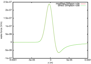
Figure 6: The CSR wakefield as a function of bunch length coordinate in an electron beam with the modified Simpson rule ($137$ grid points) and the direct Simpson rule ($8191$ grid points).

It is seen that the wakefield from the modified Simpson rule agrees with the high resolution direct Simpson rule very well even with only $137$ grid points.

IV Summary

In this paper, we present a fast high-order method for numerical calculation of the wakefield on electrons inside an electron beam. Using the Simpson quadrature rule, we present examples to calculate the wakefields from the resonator wake function and from the CSR wake function. These examples can have $O(h^{4})$ accuracy with a $O(Nlog(N))$ computational cost. Besides the fast speed and potential high numerical accuracy, the above CSR wakefield calculation also uses the direct line density instead of the first derivative of the line density with numerical filtering of the density as suggested in Reference borland . This paper gives application examples to the calculation of the longitudinal wakefield for an electron beam. The same method can also be applied to the calculation of the transverse wakefields inside an electron beam using a modified density function.

References

- (1) J. Qiang, R. D. Ryne, S. Habib, V. Decyk, J. Comp. Phys. vol. 163, 434, (2000).
- (2) J. Qiang, R. D. Ryne, M. Venturini, A. A. Zholents, I. V. Pogorelov, Phys. Rev. ST Accel. Beams, 12, 100702 (2009).
- (3) M. Borland, ANL Advanced Photon Source Report No. LS-287, 2000.
- (4) K. Bane, P. Emma, in Proc. of PAC05, p. 4266, 2005.
- (5) R. W. Hockney and J. W. Eastwood, Computer Simulation Using Particles, Adam Hilger: New York, 1988.
- (6) W. H. Press, B. P. Flannery, S. A. Teukolsky, and W. T. Vetterling,Numerical Recipes in FORTRAN: The Art of Scientific Computing, 2nd ed. Cambridge, England: Cambridge University Press, 1992.
- (7) J. Qiang, S. Lidia, R. D. Ryne, and C. Limborg-Deprey, Phys. Rev. ST Accel. Beams 9, 044204 (2006).
- (8) Robert D. Ryne, On FFT-based convolutions and correlations, with application to solving Poisson’s equation in an open rectangular pipe, arXiv:1111.4971 (2011).
- (9) J. Qiang, Comp. Phys. Comm. 18, 313316, (2010).
- (10) M. Abramowitz and I. A. Stegun, eds. Handbook of Mathematical Functions with Formulas, Graphs, and Mathematical Tables, New York: Dover, 1972.
- (11) http://mathworld.wolfram.com/Newton-CotesFormulas.html.
- (12) K. L. F. Bane, “Resistive Wall Wakefield in the LCLS Undulator Beam Pipe,” SLAC-PUB-10707, Revised October 2004.
- (13) E. L. Saldin, E. A. Schneidmiller, M. V. Yurkov, Nucl. Inst. Meth. Phys. Res. A 398, pp. 373-394, 1997.
- (14) R. D. Ryne, B. Carlsten, J. Qiang, N. Yampolsky, “A Model for One-Dimensional Coherent Synchrotron Radiation including Short-Range Effects,” arXiv:1202.2409 (2012).
- (15) J. B. Murphy, S. Krinsky, and R. L. Gluckstern, Particle Accelerators, Vol 57, pp. 9-64, 1997.
- (16) M. Borland, Phys. Rev. Sepecial Topics - Accel. Beams 4, 070701 (2001).