The Pauli equation with complex boundary conditions

Abstract

We consider one-dimensional Pauli Hamiltonians in a bounded interval with possibly non-self-adjoint Robin-type boundary conditions. We study the influence of the spin-magnetic interaction on the interplay between the type of boundary conditions and the spectrum. A special attention is paid to $\mathcal{PT}$-symmetric boundary conditions with the physical choice of the time-reversal operator $\mathcal{T}$.

• Primary: 34L40, 34B08; 81Q12; Secondary: 34B07, 81V10

• Pauli equation, spin-magnetic interaction, Robin boundary conditions, non-self-adjointness, non-Hermitian quantum mechanics, $\mathcal{PT}$-symmetry, time-reversal operator

1 Introduction

In recent years there has been a growing interest in non-Hermitian “extensions” of quantum mechanics, usually associated with the names of $\mathcal{PT}$-symmetry, pseudo-Hermiticity, quasi-Hermiticity or crypto-Hermiticity (we respectively refer to [4, 29, 31, 38] where the first two works are recent surveys with many references). The quotation marks are used here because the extended theories are physically relevant only if the operators in question are similar to self-adjoint operators, which in turn puts the concept back to the conventional quantum mechanics.

However, the freedom related to the existence of the similarity transformation can be highly useful in applications, since a complicated non-local self-adjoint operator can be represented by a (possibly non-self-adjoint) differential operator (see [23] for one-dimensional examples), and the spectral theory for the latter is much more developed. Moreover, it is necessary that the non-Hermitian operators possess real spectra, which can be often ensured (at least in some perturbative regimes [9, 27]) by the simple criterion of $\mathcal{PT}$-symmetry.

The goal of the present paper is to examine the role of spin in the above theories. We consider the simplest non-trivial situation of an electron (spin $\frac{1}{2}$, mass $m$, charge $-e<0$) interacting exclusively with an external homogeneous magnetic field $\vec{B}\in\mathbb{R}^{3}$. Choosing the Poincaré gauge in which the magnetic vector potential coincides with $\frac{1}{2}\vec{B}\times\vec{x}$, this system is governed by the Pauli equation

$$i\hbar\frac{\partial\Psi}{\partial t}=-\frac{\hbar^{2}}{2m}\,\Delta\Psi+\frac{\mu}{\hbar}\,\vec{B}\cdot\vec{L}\,\Psi+\frac{e^{2}}{8m}\,(\vec{B}\times\vec{x})^{2}\Psi+\mu\,\vec{B}\cdot\vec{\sigma}\,\Psi=:H\Psi$$ (1.1)

in the space-time variables $(\vec{x},t)$, where $\hbar$ is the reduced Planck constant, $\mu:=\hbar e/(2m)$ is the Bohr magneton (for simplicity), $\vec{L}$ is the angular-momentum operator and $\vec{\sigma}$ is a three-component vector formed by the Pauli matrices. The spinorial wavefunction $\Psi$ can be represented as an element of $L^{2}(\mathbb{R}^{3})\otimes\mathbb{C}^{2}$ and the operators appearing in (1.1) are assumed to appropriately act in this Hilbert space.

The Hamiltonian $H$ (equipped with a suitable domain) is Hermitian when considered in the full Hilbert space $L^{2}(\mathbb{R}^{3})\otimes\mathbb{C}^{2}$. Moreover, the Pauli equation (1.1) is invariant under a simultaneous reversal of the space and time variables (cf the discussion in Section 5). Relying on general definitions for the Dirac field (see, e.g., [5, §26]) and the fact that the Pauli equation can be obtained from the Dirac equation in a non-relativistic limit, the discrete symmetries can be represented by means of the parity $\mathcal{P}$ and the time-reversal operator $\mathcal{T}$ (uniquely determined up to a phase factor).

Our way how to “complexify” (1.1) is to restrict the space variables to a subset $\Omega\subset\mathbb{R}^{3}$ and impose complex boundary conditions of the Robin type

$$\frac{\partial\Psi}{\partial n}+A\Psi=0\qquad\mbox{on}\qquad\partial\Omega\,,$$ (1.2)

where $n$ is the outward pointing normal unit to $\partial\Omega$ and $A$ is a two-by-two complex-valued matrix. If $\Omega$ is invariant with respect to the spatial inversion $\mathcal{P}$, it is possible to choose $A$ in such a way that the $\mathcal{PT}$-symmetry of (1.1) remains valid for the (possibly non-Hermitian) operator $H$ on $L^{2}(\Omega)\otimes\mathbb{C}^{2}$, subject to the boundary conditions (1.2).

In this paper we study the interplay between the form of the matrix $A$ and the spectrum of $H$. In particular, we are interested in the existence of real eigenvalues in the $\mathcal{PT}$-symmetric situation.

We are not aware of previous works on Pauli equation in the non-Hermitian extensions of quantum mechanics. However, there exist results on spinorial systems in the context of $\mathcal{PT}$-symmetric coupled-channels models [35, 36, 37] and the Dirac equation in the framework of Krein spaces [1, 24].

One of the reasons for considering the spinorial model in this paper is the fact that the time-reversal operator $\mathcal{T}$ differs from the complex conjugation, the latter being the time-reversal operator for the scalar (i.e. spinless) Schrödinger equation, widely studied in the $\mathcal{PT}$-symmetric quantum theory. In fact, for fermionic systems (i.e. half-integer non-zero spin), one has

$$\mathcal{T}^{2}=-1\,.$$ (1.3)

This has been remarked previously in the context of pseudo-Hermitian operators in [32, 6]. A generalized concept of $\mathcal{PT}$-symmetry as regards the operator $\mathcal{P}$ is suggested in [34].

The present model can be regarded as an extension of the one-dimensional scalar Hamiltonians with complex Robin boundary conditions studied in [21, 20, 23] to the spinorial case. We refer to [22, 15] for the discussion of relevance of (possibly non-Hermitian) Robin boundary conditions in physics and, in particular, to Section 3 for a simple scattering-type interpretation in the present setting.

This paper is organized as follows. In the following section we specify our model in terms of a one-dimensional Hamiltonian coming from (1.1). A physical relevance of the boundary conditions (1.2) is suggested in Section 3. Section 4 is devoted to a rigorous definition of our Hamiltonian as a closed operator associated with a sectorial sesquilinear form. In Section 5 we discuss the physical choice of the operator $\mathcal{PT}$ and establish conditions on the boundary matrix $A$ which guarantee various symmetry properties of the Hamiltonian. Section 6 is devoted to a spectral analysis supported by numerics; on several $\mathcal{PT}$-symmetric examples we discuss the dependence of the spectrum on parameters characterizing the matrix $A$. The paper is concluded by Section 7 in which we mention some open problems.

2 Our model

We begin specifying our model represented by the Pauli equation (1.1).

We choose the coordinate system in $\mathbb{R}^{3}$ in such a way that the third coordinate axis is parallel with the homogeneous magnetic field $\vec{B}$, i.e. $\vec{B}=(0,0,B)$ where $B\in\mathbb{R}$. Then the orbital interaction $\vec{B}\cdot\vec{L}$ and the diamagnetic term $(\vec{B}\times\vec{x})^{2}$ represent differential operators in the first two space variables only. On the other hand, the spinorial interaction $\vec{B}\cdot\vec{\sigma}$ acts in the third space variable only (through the Pauli matrix $\sigma_{3}=\mathop{\mathrm{diag}}\nolimits(1,-1)$).

We set

$$\Omega:=\mathbb{R}^{2}\times(-a,a)\,,$$ (2.1)

with some positive number $a$. Assuming that the matrix $A$ in (1.2) is constant on each of the connected components of $\partial\Omega$, the spectral problem for the Hamiltonian $H$ therefore splits into two separate problems: a two-dimensional Landau-level problem in the first two variables and a one-dimensional problem in the third variable which we will study in sequel. Up to a constant factor representing the energy of the given Landau level, the corresponding one-dimensional operators have the form

$$H_{b}=\begin{pmatrix}-\frac{\displaystyle{{\rm d}}^{2}}{\displaystyle{{\rm d}}x^{2}}+b&0\\ 0&-\frac{\displaystyle{{\rm d}}^{2}}{\displaystyle{{\rm d}}x^{2}}-b\end{pmatrix}\qquad\mbox{on}\qquad\mathcal{H}:=L^{2}\big{(}(-a,a);\mathbb{C}^{2}\big{)}\,,$$ (2.2)

subject to the boundary conditions

$$\Psi^{\prime}(\pm a)+A^{\pm}\Psi(\pm a)=0\,.$$ (2.3)

Here we have put $\hbar^{2}/(2m)=1$ and $b:=\mu B$, $A^{\pm}\in\mathbb{C}^{2\times 2}$, and the third space variable is (with an abuse of notation) denoted by $x$.

In view of the choice of physical constants made above, the only distinguished length in our problem is the half-width $a$, and therefore the results must be scaled appropriately with respect to this length. In particular, the parameter $b$ (characterizing the strength of the magnetic field) and eigenvalues of $H_{b}$ (corresponding to quantum energies) become dimensionless when multiplied by $a^{2}$. The same can be done for the entries of $A^{\pm}$ when multiplied by $a$. Consequently, all parameters can be thought as dimensionless in the sequel.

As usual, the Hilbert space $\mathcal{H}$ is identified with $L^{2}((-a,a))\otimes\mathbb{C}^{2}$ and its elements are represented by the two-component spinors

$$\Psi=\begin{pmatrix}\psi_{+}\\ \psi_{-}\end{pmatrix}\,,$$

where $\psi_{\pm}\in L^{2}((-a,a))$ (the $\pm$ notation should not be confused with the superscripts of the matrices $A^{\pm}$ referring to the endpoints of $(-a,a)$). The inner product in $\mathcal{H}$ is defined by

$$(\Phi,\Psi):=\int_{-a}^{a}\overline{\Phi}^{T}\!(x)\,\Psi(x)\,{\rm d}x\,,$$

where the upper index $T$ denotes transposition. The corresponding norm is denoted by $\|\cdot\|$. The Euclidean norm of the spinor $\Psi$ as a vector in $\mathbb{C}^{2}$ is denoted by $|\Psi|:=\sqrt{|\psi_{+}|^{2}+|\psi_{-}|^{2}}$ and we use the same notation for the corresponding operator (matrix) norm $|A|:=\max\big{\{}|A\Psi|\,\big{|}\,\Psi\in\mathbb{C}^{2},\,|\Psi|=1\big{\}}$ for $A\in\mathbb{C}^{2\times 2}$.

3 A scattering motivation

Before giving a rigorous definition of our Hamiltonian formally introduced (2.2)–(2.3), let us first justify the physical relevance of the boundary conditions (2.3). Our method is based on a generalization of an idea originally suggested in [15].

Consider a generalized eigenvalue problem for the Hamiltonian of the form (2.2) on the whole space $\mathbb{R}$ locally perturbed by an electric field:

$$\begin{pmatrix}-\frac{\displaystyle{{\rm d}}^{2}}{\displaystyle{{\rm d}}x^{2}}+b+V(x)&0\\ 0&-\frac{\displaystyle{{\rm d}}^{2}}{\displaystyle{{\rm d}}x^{2}}-b+V(x)\end{pmatrix}\begin{pmatrix}\psi_{+}\\ \psi_{-}\end{pmatrix}=\lambda\begin{pmatrix}\psi_{+}\\ \psi_{-}\end{pmatrix}\,.$$ (3.1)

Here $x\in\mathbb{R}$, $\lambda\in\mathbb{R}$ and $V$ is the electric potential that is assumed to be compactly supported in $(-a,a)$. Solutions $\Psi$ with $\lambda<-|b|$ are bound states (associated with discrete eigenvalues), while those with $\lambda\geq-|b|$ correspond to scattering states (associated with the essential spectrum).

Outside the support of $V$ the problem (3.1) admits explicit solutions in terms of exponential functions. Let us look for special scattering solutions satisfying

$$\Psi(x)=\begin{pmatrix}e^{{\rm i}\sqrt{\lambda-b}\,x}\\ e^{{\rm i}\sqrt{\lambda+b}\,x}\end{pmatrix}\qquad\mbox{for}\qquad|x|\geq a\,.$$ (3.2)

Then the (physical) problem (3.1) on the whole real axis can be solved by considering an (effective) boundary value problem in $(-a,a)$. The latter is simply obtained by considering (3.1) in $(-a,a)$ and requiring that the solutions match at $\pm a$ smoothly with the asymptotic solutions (3.2). This leads to the boundary conditions (2.3) with an energy-dependent matrix

$$A_{\lambda}^{\pm}=\begin{pmatrix}-{\rm i}\sqrt{\lambda-b}&0\\ 0&-{\rm i}\sqrt{\lambda+b}\end{pmatrix}\,.$$ (3.3)

Note that (3.1) for $x\in(-a,a)$, subject to (2.3) with (3.3) at $\pm a$, does not represent a standard spectral problem, it is rather an operator-pencil problem (because of the dependence of $A_{\lambda}^{\pm}$ on the spectral parameter $\lambda$). It is non-linear in its nature. However, it can be solved by first considering a genuine (linear) spectral problem, namely (3.1) for $x\in(-a,a)$, subject to (2.3) with $A_{\alpha}^{\pm}$ at $\pm a$, with $\alpha$ being treated as a real parameter. This leads to a discrete set of eigencurves $\alpha\mapsto\lambda_{n}(\alpha)$, $n\in\mathbb{N}$. Then the “eigenvalues” of the true, energy-dependent problem are determined as those points $\lambda_{n}(\alpha_{*})$ satisfying the (non-linear) algebraic equations

$$\lambda_{n}(\alpha_{*})=\alpha_{*}\,.$$ (3.4)

The elements of the set $\{\lambda_{n}(\alpha_{*})\}_{n\in\mathbb{N}}$ are called perfect-transmission energies (PTEs) in [15], since their physical meaning is that they determine energies for which there is no reflection for the initial scattering problem (3.1) in $\mathbb{R}$. It is interesting that PTEs are real, although they are obtained via solving a highly non-self-adjoint spectral problem. This feature is related to the fact that the choice $A_{\alpha}^{\pm}$ ensures that the boundary conditions are $\mathcal{PT}$-symmetric (although not $\mathcal{PT}$-symmetric in the context of the present paper where we do not allow the presence of $\lambda$ and $b$ in the boundary conditions, see below). A physical interpretation of the possible complexification of the spectra of the auxiliar $\mathcal{PT}$-symmetric spectral problem is also proposed in [15].

It is also interesting to note that switching on the static magnetic field (i.e. making $b\not=0$) will typically lead to a splitting of the doubly degenerate eigencurves corresponding to the auxiliar non-self-adjoint spectral problem for $b=0$ (cf Figure 2). Consequently, to each of the PTE in the scalar case without the magnetic field there correspond two PTEs in our spinorial model. The analogy with the Zeeman effect should not be surprising.

The matrix (3.3) is complex and non-Hermitian, which is typical for effective models of scattering solutions of (3.1). On the other hand, real-valued Hermitian matrices are obtained when looking for bound states. In this paper, we proceed in a full generality by allowing arbitrary matrices $A^{\pm}$ in (2.3). However, it is important to stress that we regard the matrices as parameters entering the spectral system; the dependence of $A^{\pm}$ on the spectral parameter $\lambda$ is not allowed and the dependence on the field $b$ is allowed only if $b$ is treated as a parameter (no change under the action of $\mathcal{T}$, cf Section 5).

To end up this motivation section, let us note that alternative proposals for the connection between non-Hermitian $\mathcal{PT}$-symmetric operators and physics have been suggested recently in the context of scattering in [16, 28, 33, 17].

4 The Pauli Hamiltonian

We now turn to a rigorous definition of the Hamiltonian formally introduced by (2.2)–(2.3). In other words, since we are interested in spectral properties, we need a closed realization of the operator $H_{b}$.

The easiest way is to define the Hamiltonian as the Friedrichs extension of the operator (2.2) initially considered on uniformly smooth spinors satisfying (2.3). On such a restricted domain, an integration by parts easily leads to the associated sesquilinear form $h_{b}$ as a sum of three terms

$$h_{b}(\Phi,\Psi)=q_{1}(\Phi,\Psi)+b\,q_{2}(\Phi,\Psi)+q_{3}(\Phi,\Psi)\,,\\$$ (4.1)

where

$$q_{1}(\Phi,\Psi) :=(\Phi^{\prime},\Psi^{\prime})\,,$$ (4.2)

$$q_{2}(\Phi,\Psi) :=(\Phi,\sigma_{3}\Psi)\,,$$

$$q_{3}(\Phi,\Psi) :=\overline{\Phi}^{T}\!(a)\,A^{+}\,\Psi(a)-\overline{\Phi}^{T}\!(-a)\,A^{-}\,\Psi(-a)\,.$$

The form $h_{b}$ is well defined on a larger, Sobolev-type space

$$\mathfrak{D}(h_{b}):=H^{1}\big{(}(-a,a);\mathbb{C}^{2}\big{)}\,.$$ (4.3)

It is obvious for $q_{1}$ and $q_{2}$, while the boundary term $q_{3}$ can be shown bounded on $\mathfrak{D}(h_{b})$ by means of the Sobolev embedding $H^{1}((-a,a))\hookrightarrow C^{0}([-a,a])$.

Our aim is to show that $h_{b}$ is a closed sectorial form. It is clear for $q_{1}$ defined on (4.3), since $q_{1}$ is associated with the Neumann Laplacian (cf [10, Sec. 7]), and as such it is a densely defined, closed, symmetric, non-negative form. The term $q_{2}$ represents just a bounded perturbation; indeed, $|q_{2}[\Psi]|\leq\|\Psi\|^{2}$ for every $\Psi\in\mathcal{H}$. It is not longer true for $q_{3}$, however, a suitable quantification of the Sobolev embedding can be used to ensure that $q_{3}$ still represents a small perturbation in the following sense.

Lemma 1.

For every $\Psi\in\mathfrak{D}(h_{b})$ and $\varepsilon\in(0,1)$,

$$\big{|}q_{3}[\Psi]\big{|} \leq\varepsilon\left(|A^{+}|+|A^{-}|\right)\|\Psi^{\prime}\|^{2}+\left(\frac{|A^{+}|+|A^{-}|}{2a}+\frac{|A^{+}|+|A^{-}|}{\varepsilon}\right)\|\Psi\|^{2}\,.$$

Consequently, the form $q_{2}+q_{3}$ is relatively bounded with respect to $q_{1}$ and the relative bound can be made arbitrarily small.

Proof.

The claim is based on the estimates

$$|\Psi(\pm a)|^{2}\leq 2\;\!\|\Psi^{\prime}\|\|\Psi\|+\frac{1}{2a}\,\|\Psi\|^{2}\leq\varepsilon\,\|\Psi^{\prime}\|^{2}+\left(\frac{1}{2a}+\frac{1}{\varepsilon}\right)\|\Psi\|^{2}$$ (4.4)

valid for any $\Psi\in\mathfrak{D}(h_{b})$. Here the first inequality can be established quite easily by the fundamental theorem of calculus and the Schwarz inequality. ∎

Consequently, the perturbation result [18, Thm.VI.1.33] can be used to show that $h_{b}$ is indeed sectorial and closed. According to the first representation theorem [18, Thm.VI.2.1], there exists a unique m-sectorial operator $H_{b}$ in $\mathcal{H}$ such that $h_{b}(\Phi,\Psi)=(\Phi,H_{b}\Psi)$ for all $\Phi\in\mathfrak{D}(h_{b})$ and $\Psi\in\mathfrak{D}(H_{b})\subset\mathfrak{D}(h_{b})$. Following the arguments [18, Ex. VI.2.16], it is easy to check that $H_{b}$ indeed acts as (2.2)–(2.3); more precisely,

$$H_{b}\Psi =\begin{pmatrix}-\psi_{+}^{\prime\prime}+b\psi_{+}\\ -\psi_{-}^{\prime\prime}-b\psi_{-}\end{pmatrix},$$ (4.5)

$$\mathfrak{D}(H_{b}) =\Big{\{}\Psi\in H^{2}\big{(}(-a,a);\mathbb{C}^{2}\big{)}\ \big{|}\ \Psi^{\prime}(\pm a)+A^{\pm}\Psi(\pm a)=0\Big{\}}\,.$$

Proposition 1.

$H_{b}$ defined by (4.5) is an m-sectorial operator on $\mathcal{H}$. The adjoint of $H_{b}$ is given by

$$H_{b}^{*}\Psi =\begin{pmatrix}-\psi_{+}^{\prime\prime}+b\psi_{+}\\ -\psi_{-}^{\prime\prime}-b\psi_{-}\end{pmatrix},$$ (4.6)

$$\mathfrak{D}(H_{b}^{*}) =\Big{\{}\Psi\in H^{2}\big{(}(-a,a);\mathbb{C}^{2}\big{)}\ \big{|}\ \Psi^{\prime}(\pm a)+(A^{\pm})^{*}\;\!\Psi(\pm a)=0\Big{\}}\,,$$

where $A^{*}=\overline{A^{T}}$.

Proof.

It remains to notice (cf [18, Thm. VI.2.5]) that the adjoint operator is determined as the m-sectorial operator associated with the adjoint form $h_{b}^{*}$ defined by $h_{b}^{*}(\Phi,\Psi):=\overline{h_{b}(\Psi,\Phi)}$, $\mathfrak{D}(h_{b}^{*}):=\mathfrak{D}(h_{b})$. ∎

Note that the choice $A^{\pm}=0$ gives rise to the (self-adjoint) Pauli Hamiltonian, subject to Neumann boundary conditions, that we denote by $H_{b}^{N}$. (At the same time, the choice $A^{\pm}=\infty$ formally corresponds to Dirichlet boundary conditions.)

5 Symmetry properties

It is well known that the Pauli equation (1.1) (in the whole space $\mathbb{R}^{3}$) is invariant under the simultaneous space inversion and time reversal (i.e. $\vec{x}\mapsto-\vec{x}$ and $t\mapsto-t$, respectively). This can be easily established if one realizes that the time reversal leads to a change of orientation of the magnetic field (i.e. $\vec{B}\mapsto-\vec{B}$), while the orientation is unchanged by the space inversion. These properties can be deduced from Maxwell’s equations to which the equation (1.1) is implicitly coupled (cf [26, §17]).

One is tempted to mathematically formalize the space-time reversal invariance in terms of a symmetry property of the Hamiltonian $H$. Given a unitary or antiunitary operator $\mathcal{C}$, we say that a linear operator $H$ in a Hilbert space is $\mathcal{C}$-symmetric if

$$[H,\mathcal{C}]=0\,.$$ (5.1)

Here the commutator relation should be interpreted as an operator identity on the domain of $H$, i.e. $\mathcal{C}H\subset H\mathcal{C}$. In this framework, however, the Hamiltonian $H$ appearing (1.1) is not $\mathcal{PT}$-symmetric, just because there is no way how ensure the change of sign $\vec{B}$ under the action of $\mathcal{T}$ in the Hilbert-space setting (in which $\vec{B}$ is considered as an operator of multiplication). Nevertheless, $H$ of course satisfies (5.1) with $\mathcal{C}=\mathcal{PT}$ provided that the magnetic field is absent.

One of the goals of this section is to determine the class of boundary matrices $A^{\pm}$ which preserves the $\mathcal{PT}$-symmetry in the sense above. In other words, since we do not like to think of $b$ as a component of a field governed by the additional equations and to mathematically formalize the action of $\mathcal{T}$ on the field ($b$ is rather a fixed parameter in our Hilbert-space setting), we restrict ourselves to rigorously looking for the property

$$[H_{0},\mathcal{PT}]=0\,;$$ (5.2)

boundary conditions (2.3) satisfying this relation will be called $\mathcal{PT}$-symmetric. In other words, boundary conditions are $\mathcal{PT}$-symmetric if, and only if, $\mathcal{PT}\Psi$ satisfies the same equations as $\Psi$ in (2.3). Similarly, we shall define $\mathcal{PK}$-symmetric boundary conditions.

In our one-dimensional situation (2.2), the parity $\mathcal{P}$ and the time reversal operator $\mathcal{T}$ act on spinors as follows (cf [25, §30] and [25, §60], respectively)

$$(\mathcal{P}\Psi)(x):=\Psi(-x)\,,\qquad(\mathcal{T}\Psi)(x):=i\sigma_{2}\overline{\Psi(x)}=\begin{pmatrix}\overline{\psi_{-}(x)}\\ -\overline{\psi_{+}(x)}\end{pmatrix}\,.$$ (5.3)

It is important to stress that $\mathcal{T}$ differs from the complex conjugation operator

$$(\mathcal{K}\Psi)(x):=\overline{\Psi(x)}\,,$$ (5.4)

the latter being the time reversal operator in the scalar case.

It is easily seen that $\mathcal{P}$, $\mathcal{T}$ and $\mathcal{K}$ are norm-preserving, mutually commuting bijections on $\mathcal{H}$. $\mathcal{P}$ is linear, while $\mathcal{T}$ and $\mathcal{K}$ are antilinear (i.e. conjugate-linear) operators. $\mathcal{P}$ and $\mathcal{K}$ are involutive (i.e. $\mathcal{P}^{2}=1=\mathcal{K}^{2}$), while $\mathcal{T}$ satisfies (1.3).

Proposition 2.

$H_{0}$ is

• $\mathcal{PT}$-symmetric if, and only if, $A^{-}=\mathcal{T}A^{+}\mathcal{T}$, i.e.,

  $$A^{-}=\begin{pmatrix}-\overline{a_{22}}&\overline{a_{21}}\\ \overline{a_{12}}&-\overline{a_{11}}\end{pmatrix}\qquad\mbox{for}\qquad A^{+}=\begin{pmatrix}a_{11}&a_{12}\\ a_{21}&a_{22}\end{pmatrix}\,;$$

• $\mathcal{PK}$-symmetric if, and only if, $A^{-}=-\mathcal{K}A^{+}\mathcal{K}\equiv-\overline{A^{+}}$ , i.e.,

  $$A^{-}=\begin{pmatrix}-\overline{a_{11}}&-\overline{a_{12}}\\ -\overline{a_{21}}&-\overline{a_{22}}\end{pmatrix}\qquad\mbox{for}\qquad A^{+}=\begin{pmatrix}a_{11}&a_{12}\\ a_{21}&a_{22}\end{pmatrix}\,.$$

Proof.

Since the space $H^{2}((-a,a);\mathbb{C}^{2})$ is left invariant under the actions of $\mathcal{P}$, $\mathcal{T}$ and $\mathcal{K}$, it is enough to impose algebraic conditions on $A^{\pm}$ so that the symmetry properties are ensured. More specifically, we need to ensure that $\Psi\in\mathfrak{D}(H_{0})$ implies $\mathcal{PT}\Psi\in\mathfrak{D}(H_{0})$. Employing the identity

$$(\mathcal{PT}\Psi)^{\prime}(\pm a)+A^{\pm}(\mathcal{PT}\Psi)(\pm a) =(-\mathcal{T}\Psi)^{\prime}(\mp a)+A^{\pm}(\mathcal{T}\Psi)(\mp a)$$

$$=-\mathcal{T}\left[\Psi^{\prime}(\mp a)+\mathcal{T}A^{\pm}\mathcal{T}\Psi(\mp a)\right]$$

and the bijectivity of $\mathcal{T}$, the $\mathcal{PT}$-symmetry condition follows. The $\mathcal{PK}$-symmetry condition can be established in the same manner. ∎

Another property we would like to examine in this section is related to the notion of $S$-self-adjointness. We say that a densely defined operator $H$ on a Hilbert space is $S$-self-adjoint if

$$H^{*}=S^{-1}HS$$ (5.5)

for some bounded and boundedly invertible (possibly antilinear) operator $S$, where $H^{*}$ denotes the adjoint of $H$. It clearly generalizes the notion of self-adjointness and pseudo-Hermiticity.

Proposition 3.

$H_{0}$ is

• self-adjoint if, and only if, $(A^{\pm})^{*}=A^{\pm}\,;$

• $\mathcal{P}$-self-adjoint if, and only if, $A^{-}=-(A^{+})^{*}$, i.e.,

  $$A^{-}=\begin{pmatrix}-\overline{a_{11}}&-\overline{a_{21}}\\ -\overline{a_{12}}&-\overline{a_{22}}\end{pmatrix}\qquad\mbox{for}\qquad A^{+}=\begin{pmatrix}a_{11}&a_{12}\\ a_{21}&a_{22}\end{pmatrix}\,;$$

• $\mathcal{T}$-self-adjoint if, and only if, $(A^{\pm})^{*}=-\mathcal{T}A^{\pm}\mathcal{T}$, i.e.,

  $$A^{\pm}=\begin{pmatrix}a^{\pm}&0\\ 0&a^{\pm}\end{pmatrix}\qquad\mbox{with}\qquad a^{\pm}\in\mathbb{C}\,;$$

• $\mathcal{K}$-self-adjoint if, and only if, $(A^{\pm})^{*}=\mathcal{K}A^{\pm}\mathcal{K}\equiv\overline{A^{\pm}}\,;$

Proof.

The claims follows by using similar arguments as in the proof of Proposition 2. ∎

The spectral analysis of non-self-adjoint operators is more difficult than in the self-adjoint case, partly because the residual spectrum is in general not empty for the former. One of the goals of the present paper is to point out that the existence of this part of spectrum is always ruled out for $S$-self-adjoint operators with antilinear $S$.

Proposition 4 (General fact).

Let $H$ be a densely defined closed linear operator on a Hilbert space satisfying (5.5) with a bounded and boundedly invertible antilinear operator $S$. Then the residual spectrum of $H$ is empty.

Proof.

Since $H$ is $S$-self-adjoint, it is easy to see that $\lambda$ is an eigenvalue of $H$ (with eigenfunction $\Psi$) if, and only if, $\bar{\lambda}$ is an eigenvalue of $H^{*}$ (with eigenfunction $S^{-1}\Psi$). It is then clear from the general identity

$$\sigma_{\mathrm{r}}(H)=\left\{\lambda\in\mathbb{C}\ |\ \bar{\lambda}\in\sigma_{\mathrm{p}}(H^{*})\ \&\ \lambda\not\in\sigma_{\mathrm{p}}(H)\right\}$$

that the residual spectrum of $H$ must be empty. ∎

The proposition generalizes the fact pointed out in [7] for $S$-self-adjoint operators with $S$ being a conjugation operator (e.g. $\mathcal{K}$) and applies to our (different) choice of $\mathcal{T}$.

6 Spectral analysis

6.1 Location of the spectrum and pseudospectrum

As a consequence of Proposition 1, we know that the numerical range of $H_{b}$ is contained in a sector of the complex plane. Since the spectrum is a subset of the closure of the numerical range, it provides a basic information on the location of the spectrum of $H_{b}$. However, coming back to the inequality (4.4) on which the proof of Lemma 1 is based, we are able to establish a better result in our case.

Proposition 5.

The spectrum of $H_{b}$ is enclosed in a parabola,

$$\sigma(H_{b})\subset\Xi_{b}:=\bigg{\{}z\in\mathbb{C}\ \Big{|}\quad\Re z \geq-\left(|b|+4\,|A|^{2}+\frac{|A|}{2a}\right)=:C\,,$$

$$|\Im z| \leq\sqrt{8}\,|A|\,\sqrt{\Re z+C}+\frac{|A|}{2a}\ \bigg{\}},$$

where $|A|:=|A^{+}|+|A^{-}|$.

Proof.

By [18, Corol. VI.2.3], the numerical range of $H_{b}$ is a dense subset of the numerical range of its form $h_{b}$, the latter being defined as the set of all complex numbers $h_{b}[\Psi]$ where $\Psi$ changes over all $\Psi\in\mathfrak{D}(h_{b})$ such that $\|\Psi\|=1$. Using the first inequality of (4.4), we get

$$\Re h_{b}[\Psi] \geq q_{1}[\Psi]+b\,q_{2}[\Psi]-|q_{3}[\Psi]|$$

$$\geq\|\Psi^{\prime}\|^{2}-|b|\,\|\Psi\|^{2}-2\,|A|\,\|\Psi^{\prime}\|\,\|\Psi\|-\frac{|A|}{2a}\,\|\Psi\|^{2}$$

$$\geq\frac{1}{2}\,\|\Psi^{\prime}\|^{2}-\left(|b|+4\,|A|^{2}+\frac{|A|}{2a}\right)\|\Psi\|^{2}\,,$$

$$|\Im h_{b}[\Psi]| \leq|q_{3}[\Psi]|\leq 2\,|A|\,\|\Psi^{\prime}\|\,\|\Psi\|+\frac{|A|}{2a}\,\|\Psi\|^{2}\,,$$

for every $\Psi\in\mathfrak{D}(h_{b})$. The claim follows by combining these two estimates. ∎

Thus the resolvent set of $H_{b}$ contains the complement of $\Xi_{b}$ in $\mathbb{C}$. As a further consequence, we can establish an upper bound on the norm of the resolvent:

$$\|(H_{b}-z)^{-1}\|\leq 1/{\rm dist}\left(z,\partial\Xi_{b}\right)\qquad\text{for all}\quad z\in\mathbb{C}\setminus\Xi_{b}.$$

This result can be also interpreted as a location of the pseudospectrum of $H_{b}$, cf [11, Sec. 9.3].

Remark 1.

Note that the set $\Xi_{b}$ in Proposition 5 is not symmetric with respect to the real axis. On the other hand, if $H_{b}$ is $\mathcal{C}$-symmetric with antiunitary $\mathcal{C}$ (e.g., if $H_{b}$ is $\mathcal{PK}$-symmetric), then we a priori know that the numerical range must be symmetric with respect to the real axis and an improved version of Proposition 5 holds.

6.2 The nature of the spectrum

Since the Neumann Laplacian $H_{0}^{N}$ has compact resolvent and the relative bound in Lemma 1 can be chosen less than $1/2$ (in fact, arbitrarily small), it follows from [18, Thm. VI.3.4] that $H_{b}$ has compact resolvent as well (for any choice of $A^{\pm}$).

Proposition 6.

$H_{b}$ has a purely discrete spectrum (i.e. any point in the spectrum is an isolated eigenvalue of finite algebraic multiplicity).

Solving the eigenvalue problem $H_{b}\Psi=\lambda\Psi$ consists in constructing the fundamental system of $-\psi_{\pm}^{\prime\prime}=k_{\pm}^{2}\psi_{\pm}$ (say, in terms of sines and cosines), with $k_{\pm}:=\sqrt{\lambda\mp b}$, and subject it to the boundary conditions (2.3). This leads to the following algebraic equation for the eigenvalues $\lambda$:

$$\left[\det(A^{+})+\det(A^{-})-a_{11}^{+}a_{22}^{-}-a_{22}^{+}a_{11}^{-}\right]k_{-}k_{+}\cos(ak_{-})\cos(ak_{+})$$

$$+\left[\det(A^{+})\det(A^{-})+a_{11}^{+}a_{11}^{-}k_{-}^{2}+a_{22}^{+}a_{22}^{-}k_{+}^{2}+k_{-}^{2}k_{+}^{2}\right]\sin(ak_{-})\sin(ak_{+})$$

$$+\left[-\det(A^{+})a_{22}^{-}+a_{22}^{+}\det(A^{-})+(-a_{11}^{+}+a_{11}^{-})k_{-}^{2}\right]k_{+}\sin(ak_{-})\cos(ak_{+})$$

$$+\left[-\det(A^{+})a_{11}^{-}+a_{11}^{+}\det(A^{-})+(-a_{22}^{+}+a_{22}^{-})k_{+}^{2}\right]k_{-}\cos(ak_{-})\sin(ak_{+})$$

$$+\left(a_{21}^{+}a_{12}^{-}+a_{12}^{+}a_{21}^{-}\right)k_{-}k_{+}=0,$$ (6.1)

where $a_{ij}^{+}$ and $a_{ij}^{-}$ denote the elements of the matrices $A^{+}$ and $A^{-}$, respectively.

There are only a few choices of $A^{\pm}$ for which (6.2) admits explicit solutions. In the sequel we consider some particular situations that we analyse with help of numerical solutions.

6.3 Examples

A self-adjoint example with avoided crossings.

Let us choose

$$A^{\pm}:=\begin{pmatrix}0&{\rm i}\alpha\\ -{\rm i}\alpha&0\end{pmatrix}\,,$$ (6.2)

where $\alpha$ is a real parameter. It follows from from Proposition 3 that all the eigenvalues are real since $H_{b}$ is self-adjoint. The implicit equation for the eigenvalues takes form

$$2\alpha^{2}k_{+}k_{-}[1-\cos(2ak_{+})\cos(2ak_{-})]=-(k_{+}^{2}k_{-}^{2}+\alpha^{4})\sin(2ak_{+})\sin(2ak_{-}).$$

The dependence of eigenvalues on the parameter $\alpha$ can be seen in Figure 1. An interesting phenomenon in this figure is the approaching of a pair of eigenvalues and its subsequent moving back and slowly approaching to constant values. It should be noted that in the point of closest approach the two curves do not intersect. This avoided crossing holds for each pair of the eigenvalues.

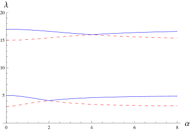
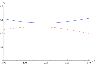
Figure 1: $\alpha$-dependence of eigenvalues for $b=1$ and $a=\frac{\pi}{4}$ in example (6.2), with a zoom of the avoided crossing of the first pair of eigenvalues on the right.

A $\mathcal{PT}$-symmetric example with real and complex spectra.

As an example of non-Hermitian but $\mathcal{PT}$-symmetric boundary conditions, let us consider

$$A^{\pm}=\begin{pmatrix}{\rm i}\alpha\pm\beta&0\\ 0&{\rm i}\alpha\pm\beta\end{pmatrix}\,,$$ (6.3)

where $\alpha$ and $\beta$ are real parameters. The feature of this example is that the spinorial components do not mix. The implicit equation for the eigenvalues acquires the form

$$\left(-2\beta k_{-}\cos(2ak_{-})+(k_{-}^{2}-\alpha^{2}-\beta^{2})\sin(2ak_{-})\right)\\ \times\left(-2\beta k_{+}\cos(2ak_{+})+(k_{+}^{2}-\alpha^{2}-\beta^{2})\sin(2ak_{+})\right)=0.$$ (6.4)

Because of the decoupling, this eigenvalue problem can be analysed by using known results for this type of boundary conditions in the scalar case previously studied in [21] and in more detail in [22]. It turns out that the spectrum significantly depends on the sign of $\beta$.

$\beta=0$. It follows from [21] that one pair of eigenvalues depend on the parameter $\alpha$ quadratically and the others are constant, see the left part of Figure 2. More specifically, the eigenvalues explicitly read

$$\lambda_{j,\pm}=\begin{cases}\alpha^{2}\mp b&\mbox{if}\quad j=0\,,\\ \left(\frac{\displaystyle j\pi}{\displaystyle 2a}\right)^{2}\mp b&\mbox{if}\quad j\geq 1\,.\end{cases}$$ (6.5)

The crossings of full (respectively dashed) lines in the left part of Figure 2 correspond to eigenvalues of geometric multiplicity one and algebraic multiplicity two, while the crossings of full lines with dashed lines correspond to eigenvalues of both multiplicities equal to two. The entire spectrum is doubly degenerate for $b=0$ and there exist eigenvalues of geometric multiplicity two and algebraic multiplicity four.

$\beta>0$. In this case, the reality of the spectrum was proved in [22]. The right part of Figure 2 shows the dependence of the eigenvalues on the parameter $\alpha$. We again observe pairs of eigenvalues split because of the presence of the magnetic field.

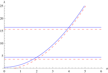
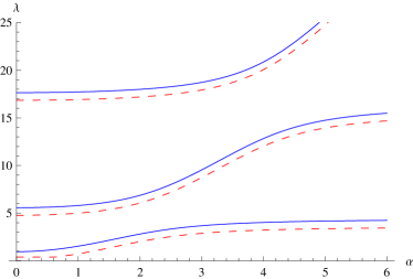
$\beta=0$	$\beta=0.5$

Figure 2: $\alpha$-dependence of eigenvalues for $b=0.4$ and $a=\frac{\pi}{4}$ in example (6.3).

$\beta<0$. On the other hand, the reality of the spectrum in the case when $\beta$ is negative is not guaranteed and, indeed, it is easily seen from Figure 3 that complex conjugate pairs of eigenvalues do appear when a couple of real eigenvalues collides as enlarging $\alpha$. The pair of complex eigenvalues becomes real again for larger values of $\alpha$. It follows from the analysis in [22] that only one pair of complex conjugate eigenvalues occurs simultaneously in the spectrum.

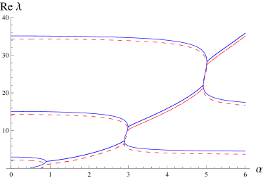
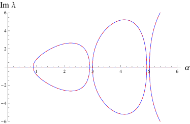
Figure 3: $\alpha$-dependence of the real (left) and imaginary (right) parts of eigenvalues for $b=0.4$, $a=\frac{\pi}{4}$ and $\beta=-0.5$ in example (6.3).

A $\mathcal{PT}$-symmetric example with coupled spinorial components

As another example of non-Hermitian $\mathcal{PT}$-symmetric boundary conditions, let us select

$$A^{\pm}=\begin{pmatrix}0&\pm{\rm i}\alpha\\ \pm{\rm i}\alpha&0\end{pmatrix},$$ (6.6)

where $\alpha$ is a real parameter. The characteristic feature of this model is a non-trivial mixing of spinorial components. The implicit equation for the eigenvalues now takes the form

$$4\alpha^{2}k_{+}k_{-}\cos(ak_{+})^{2}\cos(ak_{-})^{2} +4\alpha^{2}k_{+}k_{-}\sin(ak_{+})^{2}\sin(ak_{-})^{2}$$ (6.7)

$$=-(k_{+}k_{-}+\alpha^{4})\sin(2ak_{+})\sin(2ak_{-}).$$

The dependence of low-lying eigenvalues on the parameter $\alpha$ can be seen in Figure 4. Here the lowest pair of real eigenvalues exhibits a crossing, however, the eigenvalues remain real after the crossing point as the parameter $\alpha$ increases. This behaviour is not featured uniquely by the lowest pair of eigenvalues, it also appears for higher-lying eigenvalues in the spectrum (not visible in the figure). On the other hand, as $\alpha$ increases, the other pairs of eigenvalues in the figure complexify after the first collision, then the corresponding eigenvalues propagate as complex conjugate pairs in the complex plane, meet again and become real.

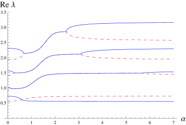
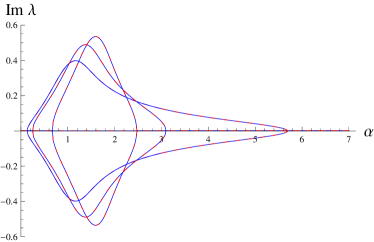
Figure 4: $\alpha$-dependence of eigenvalues for $b=0.5$, $a=\sqrt{43}$ in example (6.6). An animation can be found on the website [19].

7 Conclusions

The goal of this paper was to investigate the role of spin in complex extensions of quantum mechanics on a simple model of Pauli equation with complex Robin-type boundary conditions. A special attention was paid to $\mathcal{PT}$-symmetric situations with a physical choice of the time-reversal operator $\mathcal{T}$.

A simple physical interpretation of our model in terms of scattering was suggested in Section 3. It would be desirable to examine this motivation in more details and include “spin-dependent electric potential” (e.g. Bychkov-Rashba or Dreselhauss spin-orbit terms typical for semiconductor physics [14]).

Robin boundary conditions represent a class of separated boundary conditions. Our model can be naturally extended to connected boundary conditions, whose spectral analysis represents a direction of potential future research (cf [22, 12, 13] in the scalar case).

In this paper we did not discuss the important question of the existence of similarity transformations (or the “metric” in the $\mathcal{PT}$-symmetric context) connecting our non-Hermitian operators with self-adjoint Hamiltonians. The problem generally constitutes a difficult task and very few closed formulae are known (cf [20, 3, 2, 23] and references therein). However, we can easily extend the results established in the scalar case without magnetic field [23] to our spinorial example (6.3) and compute the metric in this special case. Let us define

$$\Theta:=\begin{pmatrix}I+K&0\\ 0&I+K\end{pmatrix}\,,$$

where $I$ denotes the identity operator on $L^{2}((-a,a))$ and $K$ is an integral operator with kernel

$$K(x,y):=e^{{\rm i}\alpha(x-y)-\beta|x-y|}\,\big{[}c+{\rm i}\alpha\mathop{\mathrm{sgn}}\nolimits(x-y)\big{]}\,,$$

with $c$ being any real number. It follows from [23, Sec. 4.5] and the nature of the decoupled boundary conditions (6.3) that $\Theta$ represents a one-parametric family of metrics for $H_{b}$ under the $\mathcal{PT}$-symmetric choice (6.3). More precisely, $H_{b}$ is $\Theta^{-1}$-self-adjoint (cf (5.5)) and $\Theta$ is positive provided that either: $a$ is small; or $\beta$ is positive and large; or $|c|$ and $|\alpha|$ are small. To find the self-adjoint counterpart of $H_{b}$ determined by this similarity transformation constitutes an open problem (in the scalar case [23] there exists results for $\beta=0$).

Our model was effectively one-dimensional. Higher dimensional generalizations in the spirit of [7, 8, 30] would be especially interesting for variable boundary conditions (i.e. non-constant matrix $A$).

Acknowledgement

The last three authors acknowledge the hospitality of the Comenius University in Bratislava where this work was initiated; these authors have been partially supported by the GACR grant No. P203/11/0701. The first author acknowledges support from DFG SFB-689. The last author has been supported by a grant within the scope of FCT’s project PTDC/MAT/101007/2008 and partially supported by FCT’s projects PTDC/MAT/101007/2008 and PEst-OE/ MAT/UI0208/2011.

References

- [1] S. Albeverio, U. Guenther, and S. Kuzhel, -self-adjoint operators with -symmetries: extension theory approach, J. Phys. A: Math. Theor. 42 (2009), 105205.
- [2] P. E. G Assis, Metric operators for non-Hermitian quadratic Hamiltonians, J. Phys. A: Math. Theor. 44 (2011), 265303.
- [3] P. E. G Assis and A. Fring, Non-Hermitian Hamiltonians of Lie algebraic type, J. Phys. A: Math. Theor. 42 (2009), 015203.
- [4] C. M. Bender, Making sense of non-Hermitian Hamiltonians, Rep. Prog. Phys. 70 (2007), 947–1018.
- [5] V. B. Berestetskii, E. M. Lifschitz, and L. P. Pitaevskii, Quantum electrodynamics, Pergamon Press, 2nd edition, 1982.
- [6] A. Blasi, G. Scolarici, and L. Solombrino, Pseudo-Hermitian Hamiltonians, indefinite inner product spaces and their symmetries, J. Phys. A: Math. Gen. 37 (2004), 4335.
- [7] D. Borisov and D. Krejčiřík, -symmetric waveguides, Integral Equations Operator Theory 62 (2008), no. 4, 489–515.
- [8] , The effective Hamiltonian for thin layers with non-Hermitian Robin-type boundary conditions, Asympt. Anal. 76 (2012), 49–59.
- [9] E. Caliceti, S. Graffi, and J. Sjöstrand, Spectra of PT-symmetric operators and perturbation theory, J. Phys. A 38 (2005), 185–193.
- [10] E. B. Davies, Spectral theory and differential operators, Camb. Univ Press, Cambridge, 1995.
- [11] , Linear operators and their spectra, Camb. Univ Press, Cambridge, 2007.
- [12] E. Ergun, A two-parameter family of non-Hermitian Hamiltonians with real spectrum, J. Phys. A: Math. Theor. 43 (2010), 455212.
- [13] E. Ergun and M. Saglam, On the metric of a non-Hermitian model, Rep. Math. Phys. 65 (2010), 367–378.
- [14] J. Fabian, A. Matos-Abiague, C. Ertler, P. Stano, and I. Žutić, Semiconductor spintronics, Acta Phys. Slovaca 67 (2007), 565–907.
- [15] H. Hernandez-Coronado, D. Krejčiřík, and P. Siegl, Perfect transmission scattering as a -symmetric spectral problem, Phys. Lett. A 375 (2011), 2149–2152.
- [16] L. Jin and Z. Song, A physical interpretation for the non-Hermitian Hamiltonian, J. Phys. A: Math. Theor. 44 (2011), 375304.
- [17] H. F. Jones, Analytic results for a -symmetric optical structure, preprint on arXiv:1111.2041v1 [physics.optics] (2011).
- [18] T. Kato, Perturbation theory for linear operators, Springer-Verlag, Berlin, 1966.
- [19] D. Kochan, D. Krejčiřík, R. Novák, and P. Siegl, http://gemma.ujf.cas.cz/~david/KKNS.html (2012).
- [20] D. Krejčiřík, Calculation of the metric in the hilbert space of a -symmetric model via the spectral theorem, J. Phys. A: Math. Theor. 41 (2008), 244012.
- [21] D. Krejčiřík, H. Bíla, and M. Znojil, Closed formula for the metric in the Hilbert space of a -symmetric model, J. Phys. A 39 (2006), 10143–10153.
- [22] D. Krejčiřík and Siegl, -symmetric models in curved manifolds, J. Phys. A: Math. Theor. 43 (2010), 485204.
- [23] D. Krejčiřík, P. Siegl, and Železný, On the similarity of Sturm-Liouville operators with non-Hermitian boundary conditions to self-adjoint and normal operators, preprint on arXiv:1108.4946 [math.SP] (2011).
- [24] S. Kuzhel and C. Trunk, On a class of -self-adjoint operators with empty resolvent set, J. Math. Anal. Appl. 379 (2011), 272–289.
- [25] L. D. Landau and E. M. Lifschitz, Quantum mechanics: Non-relativistic theory, Pergamon Press, 3rd edition, 1977.
- [26] , The classical theory of fields, Butterworth Heinemann, 4th edition, 1980.
- [27] H. Langer and Ch. Tretter, A Krein space approach to PT-symmetry, Czech. J. Phys. 54 (2004), 1113–1120.
- [28] S. Longhi, Invisibility in -symmetric complex crystals, J. Phys. A: Math. Theor. 44 (2011), 485302.
- [29] A. Mostafazadeh, Pseudo-Hermitian representation of quantum mechanics, Int. J. Geom. Meth. Mod. Phys. 7 (2010), 1191–1306.
- [30] O. Olendski, Resonant alteration of propagation in guiding structures with complex Robin parameter and its magnetic-field-induced restoration, Ann. Phys. 326 (2011), 1479–1500.
- [31] F. G. Scholtz, H. B. Geyer, and F. J. W. Hahne, Quasi-Hermitian operators in quantum mechanics and the variational principle, Ann. Phys 213 (1992), 74–101.
- [32] G. Scolarici and L. Solombrino, Pseudo-Hermitian Hamiltonians, time-reversal invariance and Kramers degeneracy, Phys. Lett. A 303 (2002), 239–242.
- [33] G. Yoo, H.-S. Sim, and H. Schomerus, Quantum noise and mode nonorthogonality in non-Hermitian PT-symmetric optical resonators, Phys. Rev. A 84 (2011), 063833.
- [34] M. Znojil, A generalization of the concept of -symmetry, Quantum Theory and Symmetries (E. Kapuscik and A. Horzela, eds.), World Scientific, Singapore, 2011, pp. 626–631.
- [35] , Coupled-channel version of -symmetric square well, J. Phys. A: Math. Gen. 39 (2006), 441–455.
- [36] , Exactly solvable models with -symmetry and with an asymmetric coupling of channels, J. Phys. A: Math. Gen. 39 (2006), 4047–4061.
- [37] , Strengthened -symmetry with †, Phys. Lett. A 353 (2006), 463–468.
- [38] , Time-dependent version of cryptohermitian quantum theory, Phys. Rev. D 78 (2008), 085003.