Non-Parametric Approximations for Anisotropy Estimation in Two-dimensional Differentiable Gaussian Random Fields

Abstract

Spatially referenced data often have autocovariance functions with elliptical isolevel contours, a property known as geometric anisotropy. The anisotropy parameters include the tilt of the ellipse (orientation angle) with respect to a reference axis and the aspect ratio of the principal correlation lengths. Since these parameters are unknown a priori, sample estimates are needed to define suitable spatial models for the interpolation of incomplete data. The distribution of the anisotropy statistics is determined by a non-Gaussian sampling joint probability density. By means of analytical calculations, we derive an explicit expression for the joint probability density function of the anisotropy statistics for Gaussian, stationary and differentiable random fields. Based on this expression, we obtain an approximate joint density which we use to formulate a statistical test for isotropy. The approximate joint density is independent of the autocovariance function and provides conservative probability and confidence regions for the anisotropy parameters. We validate the theoretical analysis by means of simulations using synthetic data, and we illustrate the detection of anisotropy changes with a case study involving background radiation exposure data. The approximate joint density provides (i) a stand-alone approximate estimate of the anisotropy statistics distribution (ii) informed initial values for maximum likelihood estimation, and (iii) a useful prior for Bayesian anisotropy inference.

1 Introduction

Fast and accurate methods of anisotropy estimation are needed in various fields to better model spatially extended processes and the properties of heterogeneous materials (Guilleminot and Soize, 2012). The characterization and measurement of anisotropy in biological tissues, for example, is important for diagnostic and medical reasons (Ranganathan et al., 2011; Richard and Bierme, 2010). Significant changes in anisotropy over time may suggest a crucial change in the underlying physical processes. For example, an accidental release of radioactivity may significantly alter the anisotropy of radioactivity patterns over the monitored area. Reliable and computationally fast detection of systematic changes in spatial distributions is crucial, especially for automatic monitoring systems (Pebesma et al., 2011). Another practical question is what constitutes a significant departure from isotropy to necessitate the use of anisotropic autocovariance functions. Non-parametric methods attempt to provide answers to such questions without requiring knowledge of the autocovariance functions (henceforward, covariance function for simplicity). Non-parametric isotropy tests are thoroughly reviewed in a recent publication (Weller and Hoeting, 2015).

Two types of anisotropy are usually encountered in spatially extended processes. Physical anisotropy implies tensor fields that represent directionally dependent material properties such as transport coefficients in heterogeneous media, e.g. (Adler, 1992). Statistical anisotropy characterizes scalar processes (e.g., scalar permeability, pollutant concentrations), the correlation range of which depends on the spatial direction. Geostatistical analysis employs two types of statistical anisotropy: geometric and zonal (Zimmerman, 1993; Chilès and Delfiner, 2012). Herein we focus on geometric anisotropy, which implies SRFs with covariance functions that possess elliptical isolevel contours (see Fig. 1). The estimation of anisotropy parameters is a topic of ongoing interest in various engineering fields (Jiang, 2005; Okada et al., 2005; Feng et al., 2008; Olhede, 2008; Le Bihan et al., 2001; Xu and Choi, 2009; Richard and Bierme, 2010; Wang and Leckie, 2012) and in data assimilation (Weaver and Mirouze, 2013). In geostatistics, the anisotropy is typically modeled by estimating the empirical variogram in different directions and fitting anisotropic variogram models (Chilès and Delfiner, 2012). For second-order stationary SRFs the variogram is equivalent to the covariance function. However, the interpretation of such variogram analysis is not always straightforward (Weller and Hoeting, 2015). Anisotropic modeling in the Bayesian framework has also been investigated (Ecker and Gelfand, 1999, 2003). Recently, there is interest in anisotropic models with locally varying parameters (Lillah and Boisvert, 2015). A study focusing on general characterizations of anisotropy beyond the geometrical model appears in (Allard et al., 2015).

The mathematical framework for the study of anisotropy in spatial processes is based on spatial random fields (SRFs), also known as spatial random functions (Adler, 1981; Christakos, 1992; Wackernagel, 1997; Lantuéjoul, 2002). SRFs are used in several scientific and engineering disciplines that study spatially distributed processes (e.g., image processing, theory of transport in heterogeneous media, wave propagation in random media, environmental modeling). SRFs with Gaussian joint probability density function also provide the mathematical framework of Gaussian processes in machine learning. Spatially referenced data are typically modeled as SRFs. The analysis of SRFs based on data involves a number of distributional assumptions that need to be validated. A common assumption is that of statistical stationarity which states that the statistical properties are independent of the position. The less strict second-order stationarity assumption is used in practice and requires the expectation of the field to be constant and the covariance function to depend only on the spatial lag. In the case of Gaussian random fields, second-order stationarity is equivalent to strong stationarity. Isotropy is a stricter assumption that requires the covariance function to depend only on the magnitude but not on the direction of the lag. For convenience, isotropic SRF models are often used, even though many real data sets display anisotropic patterns.

In the case of two-dimensional SRFs that admit first-order derivatives in the mean-square sense, a non-parametric and non-iterative method for semi-analytic estimation of anisotropy parameters was proposed and studied in (Hristopulos, 2002; Chorti and Hristopulos, 2008). This manuscript extends the works above by investigating the joint dependence of the anisotropy parameter estimates. We derive a non-parametric approximation of the sampling joint probability density function (JPDF) of anisotropy statistics for differentiable, stationary Gaussian SRFs. We prove this expression using the Covariance Hessian Identity (CHI) (Swerling, 1962), the Central Limit Theorem, Jacobi’s multivariate transformation theorem, and perturbation analysis.

The non-parametric approximation yields a sampling JPDF which is more dispersed in parameter space than the exact JPDF. This implies wider probability regions for the anisotropy parameter statistics and confidence regions for the anisotropy population parameters. Hence, if a sample is classified as isotropic at confidence level $p$ based on the approximate JPDF, it is actually isotropic at $p^{\prime}>p$. The JPDF that we derive can also be used as a prior in Bayesian model inference (Ecker and Gelfand, 1999, 2003; Schmidt and O’Hagan, 2003; Zhang, 2012) or as a preliminary step in copula-based spatial analysis (Kazianka, 2013).

This manuscript is structured as follows: In Section 2 we present essential definitions and an overview of CHI. In Section 3 we derive a general expression for the joint probability density $f_{\hat{R},\hat{\theta}}(R,\theta)$ for the anisotropy statistics $(\hat{R},\hat{\theta})$. In addition, we obtain a relation for $p$-level probability regions of the anisotropy parameters. In Section 4, we derive the non-parametric approximation of $f_{\hat{R},\hat{\theta}}(R,\theta)$ and the corresponding probability region expression. In Section 5 we formulate a non-parametric test for isotropy. In Section 6, we validate the theoretical results with numerical simulations and we illustrate the detection of anisotropy changes with a case study involving radiation exposure data. Finally, in Section 7 we review the main results obtained in this work, we present our conclusions, and we outline directions for future research. Proofs of theorems and lemmas are given in the Appendices.

2 Preliminaries

We use boldface symbols for vectors, matrices and tensors; the superscript “t” denotes the vector or matrix transpose. ${\cal D}\subset\mathbb{R}^{2}$ denotes the spatial domain, $|{\cal D}|$ the enclosed area, $\bm{\mathrm{s}}\in{\cal D}$ the position vector in ${\cal D}$, and $\|\bm{\mathrm{s}}\|$ the Euclidean norm of $\bm{\mathrm{s}}$. $X(\bm{\mathrm{s}},\omega)$ represents a scalar SRF on the probability space $(\Omega,\mathcal{F,P})$. The state index $\omega$ determines the field state and is suppressed in the following for the sake of brevity. The events in $\mathcal{F}$ comprise the measured SRF realization(s) or sample state(s). ${\mathbb{E}}\left[\cdot\right]$ denotes the expectation over the ensemble of states, and $\operatorname{Cov}\left(Z_{1},Z_{2}\right)={\mathbb{E}}\left[Z_{1}Z_{2}\right]-{\mathbb{E}}\left[Z_{1}\right]{\mathbb{E}}\left[Z_{2}\right]$ is the covariance of the random variables $Z_{1}$ and $Z_{2}$. Realizations of an SRF $X(\bm{\mathrm{s}})$ will be denoted by $x(\bm{\mathrm{s}})$.

We focus on wide-sense stationary Gaussian SRFs (GSRFs) with constant mean $m={\mathbb{E}}\left[X(\bm{\mathrm{s}})\right]$ and covariance function $c(\bm{\mathrm{r}})={\mathbb{E}}\left[X(\bm{\mathrm{s}})\,X(\bm{\mathrm{s}}+\bm{\mathrm{r}})\right]-m^{2}$. We assume that the SRF is first-order differentiable in the mean square sense for every $\bm{\mathrm{s}}\in{\cal D}$, so that the partial derivatives ${\partial^{2}c(\bm{\mathrm{r}})}/{\partial r_{i}^{2}}$ in the orthogonal directions $i=1,2$ exist at $\bm{\mathrm{r}}=(0,0)$. For Gaussian SRFs, mean square differentiability essentially implies that the respective derivatives of the sample states exist almost surely (Adler, 1981; Yaglom, 1987). We assume short-range correlations, i.e., with a finite correlation area $\int d{\bf r}\,|c({\bf r})|$. Such correlation functions have a finite integral range.

The sample, ${\bf x}_{k}=(x_{1},\ldots,x_{N})^{t}$ comprises the values $x_{k}=x(\bm{\mathrm{s}}_{k})$ of the realization $x(\bm{\mathrm{s}})$, where $\bm{\mathrm{s}}_{k},\,k=1,\dots,N$ are sampling locations. We use the following notation for the anisotropic parameters, illustrated in terms of the anisotropic ratio: population parameters are marked by a star, i.e., ${R}^{\ast}$. The sampling function of ${R}^{\ast}$ is the random variable $\hat{R}$. Specific numerical values will be denoted by $R$. Sampling functions based on discrete approximations of derivatives are denoted by $\check{R}$. The population anisotropy parameters are illustrated in Fig. 1.

The Covariance Hessian Matrix $\bm{\mathrm{H}}(\bm{\mathrm{r}})$ (CHM) of a stationary, at least first-order differentiable, SRF $X(\bm{\mathrm{s}})$ is defined as follows

$$H_{ij}(\bm{\mathrm{r}})\doteq-\frac{\partial^{2}c(\bm{\mathrm{r}})}{\partial r_{i}\,\partial r_{j}},\quad i,j=1,2.$$ (1)

Let $X_{ij}(\bm{\mathrm{s}})=\partial_{i}X(\bm{\mathrm{s}})\,\partial_{j}X(\bm{\mathrm{s}})$, $i=1,2$ be the gradient tensor, where $\partial_{i}X(\bm{\mathrm{s}})=\partial_{i}X(\bm{\mathrm{s}})/\partial s_{i}$, $i=1,2$ are the partial derivatives of $X(\bm{\mathrm{s}})$. The mean gradient tensor $\bm{\mathrm{{Q}^{\ast}}}$, also known as the matrix of spectral moments (Adler, 1981), is defined as follows

$${Q}^{\ast}_{ij}\doteq{\mathbb{E}}\left[\partial_{i}X(\bm{\mathrm{s}})\,\partial_{j}X(\bm{\mathrm{s}})\right]={\mathbb{E}}\left[X_{ij}(\bm{\mathrm{s}})\right].$$ (2)

The matrix $\bm{\mathrm{{Q}^{\ast}}}$ is nonnegative definite as the covariance of the random gradient $\nabla X(\bm{\mathrm{s}})=\left(\partial_{1}X(\bm{\mathrm{s}}),\partial_{2}X(\bm{\mathrm{s}})\right)^{t}$. It satisfies the following theorem (Swerling, 1962):

Theorem 1 (Swerling’s CHI).

Let $X(\bm{\mathrm{s}})$ be a statistically stationary SRF with covariance function $c(\bm{\mathrm{r}})$ that admits partial derivatives ${\partial^{2}c(\bm{\mathrm{r}})}/{\partial r_{i}^{2}}$ at $\bm{\mathrm{r}}=(0,0)$. Then

$$\bm{\mathrm{{Q}^{\ast}}}=\left.\bm{\mathrm{H}}(\bm{\mathrm{r}})\right|_{\bm{\mathrm{r}}=\bm{\mathrm{0}}}.$$ (3)

To define the anisotropy parameters, consider a coordinate system aligned with the principal axes of anisotropy, e.g., $A_{1}$ and $A_{2}$ (see Fig. 1). In the principal system, $c({\bf u})=\phi({\bf u}^{t}{\bf V}{\bf u})$, where ${\bf u}=(u_{1},u_{2})$ is the lag, $\bm{\mathrm{V}}$ is a diagonal $2\times 2$ matrix, and $\varphi(\cdot)$ is a positive definite function.

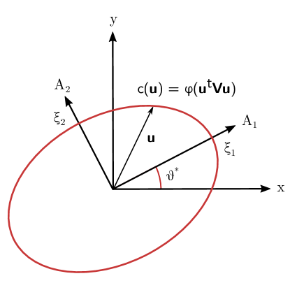
Figure 1: Definition of elliptical anisotropy parameters. The ellipse denotes an iso-level contour of an anisotropic covariance function $c(\cdot)$. The principal correlation lengths are $\xi_{1},\xi_{2}$; $R^{\ast}=\xi_{2}/\xi_{1}$ is the anisotropy ratio, while the $x$-axis and $A_{1}$ are the sides of the anisotropy angle $\theta^{\ast}$. An anisotropic covariance function $c(\cdot)$ is obtained from a positive definite function $\varphi(\cdot)$ via a rescaling $\bm{\mathrm{V}}$ followed by a rotation by $\theta^{\ast}$.

The principal correlation lengths of $X({\bm{\mathrm{s}}})$ are given by $\xi^{-2}_{i}=-a\sigma^{-2}\,\partial^{2}c({\bf u})/\partial{u}_{i}^{2}|_{\bf u={\bf 0}}$, for $i=1,2$ where $a$ is a positive constant (Chorti and Hristopulos, 2008). We define the anisotropy ratio as ${R}^{\ast}=\xi_{2}/\xi_{1}$, and the orientation (rotation) angle ${\theta}^{\ast}$ as the angle between the horizontal axis of the reference system and $A_{1}$. The anisotropy parameters $({R}^{\ast},{\theta}^{\ast})$ satisfy the following theorem:

Theorem 2.

Let $X({\bm{\mathrm{s}}})$ be an SRF satisfying the conditions of Theorem 1, and $q_{\rm d}$, $q_{\rm o}$ represent the following ratios of gradient tensor elements ${Q}^{\ast}_{ij}$:

$$q_{\mathrm{d}}^{\ast}\doteq\frac{{Q}^{\ast}_{22}}{{Q}^{\ast}_{11}}={\frac{1+{{R}^{\ast}}^{2}\tan^{2}{\theta}^{\ast}}{{{R}^{\ast}}^{2}+\tan^{2}{\theta}^{\ast}}},$$ (4a)

$$q_{\mathrm{o}}^{\ast}\doteq\frac{{Q}^{\ast}_{12}}{{Q}^{\ast}_{11}}=\frac{\tan{\theta}^{\ast}({{R}^{\ast}}^{2}-1)}{{{R}^{\ast}}^{2}+\tan^{2}{\theta}^{\ast}}.$$ (4b)

Then, the anisotropic ratio, ${R}^{\ast}$ and the orientation angle, ${\theta}^{\ast}$ are given by

$${\theta}^{\ast} =\frac{1}{2}\tan^{-1}\bigg{(}\frac{2q_{\mathrm{o}}^{\ast}}{1-q_{\mathrm{d}}^{\ast}}\bigg{)},$$ (5a)

$${R}^{\ast} =\left[1+\frac{1-q_{\mathrm{d}}^{\ast}}{q_{\mathrm{d}}^{\ast}-(1+q_{\mathrm{d}}^{\ast})\cos^{2}{\theta}^{\ast}}\right]^{-1/2}.$$ (5b)

The proof is based on Theorem 1 (Chorti and Hristopulos, 2008). Therein the notation $R=R_{2(1)}=\xi_{1}/\xi_{2}$ was used, whereas above we defined ${R}^{\ast}=\xi_{2}/\xi_{1}$. The equations (4) and (5) follow from (Chorti and Hristopulos, 2008) by means of the transformation $R\mapsto 1/{R}^{\ast}$.

Equations (4) are invariant under the pair of transformations $\tan{\theta}^{\ast}\mapsto-(\tan{\theta}^{\ast})^{-1}$, that is, ${\theta}^{\ast}\mapsto{\theta}^{\ast}\pm\pi/2,$ and ${R}^{\ast}\mapsto 1/{R}^{\ast}$. By restricting the parameter space to ${R}^{\ast}\in[0,\infty)$ and ${\theta}^{\ast}\in[-\pi/4,\pi/4)$, or equivalently to ${R}^{\ast}\in[1,\infty)$ and ${\theta}^{\ast}\in[-\pi/2,\pi/2)$, ensures that the mapping $(q_{\mathrm{d}}^{\ast},q_{\mathrm{o}}^{\ast})\mapsto({R}^{\ast},{\theta}^{\ast})$ is one-to-one, except for the point $(1,0)$ which maps to $(1,{\theta}^{\ast})$ ${\theta}^{\ast}$ being any angle $\in[-\pi/2,\pi/2)$. Theorem 2 permits estimating the anisotropy parameters without knowledge of the covariance function, if $\bm{\mathrm{{Q}^{\ast}}}$ can be estimated from the data (Hristopulos, 2002; Chorti and Hristopulos, 2008).

3 Sampling Joint PDF of Anisotropy Statistics

Every realization $x(\bm{\mathrm{s}})$ yields a different estimate of $\bm{\mathrm{{Q}^{\ast}}}$, leading to a probability distribution for the statistics $\hat{R}$ and $\hat{\theta}$. Below we derive the joint PDF $f_{\hat{R},\hat{\theta}}(R,\theta)$ based on Jacobi’s theorems for the transformation of a multivariate probability distribution under transformation of the respective variables (Papoulis and Pillai, 2002) and the Central Limit Theorem (CLT).

We estimate ${{Q}^{\ast}}_{ij}$ using the spatially averaged gradient tensor $\hat{Q}_{ij}$, where $i,j=1,2$,

$$\hat{Q}_{ij}:=\frac{1}{N}\sum_{k=1}^{N}{X}_{ij}(\bm{\mathrm{s}}_{k})=\frac{1}{N}\sum_{k=1}^{N}{\partial}_{i}{X}(\bm{\mathrm{s}}_{k})\,{\partial}_{j}{X}(\bm{\mathrm{s}}_{k}).$$ (6)

The estimation of the field’s partial derivatives from the data is discussed in Section 6. Replacing the expectation with the spatial average requires the ergodic hypothesis. A necessary condition for ergodicity is that $|\mathcal{D}|\to\infty$ in such a way that both ratios of domain length over the correlation length in the respective direction tend to infinity. In practice, this means that for an accurate estimate of ${{Q}^{\ast}}_{ij}$ the domain length along each principal direction should be considerably larger than the respective correlation length. In the following, we assume that the asymptotic regime is defined by $|\mathcal{D}|\to\infty$ in the sense defined above for ergodicity and $N\to\infty$ (for application of the CLT).

3.1 Joint PDF of Gradient Tensor Components

We define the following random vector

$${\hat{\mathbb{Q}}}=(\hat{Q}_{11},\hat{Q}_{22},\hat{Q}_{12})^{t}=\left(\frac{1}{N}\sum_{k=1}^{N}{X}_{11}(\bm{\mathrm{s}}_{k}),\,\frac{1}{N}\sum_{k=1}^{N}{X}_{22}(\bm{\mathrm{s}}_{k}),\,\frac{1}{N}\sum_{k=1}^{N}{X}_{12}(\bm{\mathrm{s}}_{k})\right)^{t},$$ (7)

that comprises the independent components of the fully symmetric gradient tensor sampling function $(\hat{Q}_{12}=\hat{Q}_{21})$. As we show below, $\hat{\mathbb{Q}}$ tends to follow the joint Gaussian distribution in the asymptotic limit due to the Central limit theorem.

According to (6), $\hat{Q}_{ij}=\frac{1}{N}\sum_{k=1}^{N}X_{ij}(\bm{\mathrm{s}}_{k})$ and based on the definition (2) it follows that ${\mathbb{E}}\left[\hat{Q}_{ij}\right]={Q}^{\ast}_{ij}$, i.e., $\hat{\mathbb{Q}}$ is an unbiased estimator of $\bm{\mathrm{{Q}^{\ast}}}$. By definition, the covariance matrix $\bm{\mathrm{C}}_{\hat{\mathbb{Q}}}$ is symmetric, namely $C_{ij;kl}=C_{kl,ij}$; hence, it involves six independent entries.

Lemma 1 (Covariance matrix $\bm{\mathrm{C}}_{\hat{\mathbb{Q}}}$).

For a statistically stationary GSRF, the six independent entries of $\bm{\mathrm{C}}_{\hat{\mathbb{Q}}}$ are given by the following series

$$C_{ij;kl} =\frac{1}{N^{2}}\sum_{\bm{\mathrm{r}}_{nm}}C_{ij;kl}(\bm{\mathrm{r_{nm}}})=\frac{1}{N^{2}}\sum_{\bm{\mathrm{r}}_{nm}}\left[H_{ik}(\bm{\mathrm{r}}_{nm})H_{jl}(\bm{\mathrm{r}}_{nm})+H_{il}(\bm{\mathrm{r}}_{nm})H_{jk}(\bm{\mathrm{r}}_{nm})\right]\!$$

$$=\frac{1}{N}\left[{Q}^{\ast}_{ik}\,{Q}^{\ast}_{jl}+{Q}^{\ast}_{il}\,{Q}^{\ast}_{jk}\right]$$

$$+\frac{1}{N^{2}}\sum_{\bm{\mathrm{r}}_{nm}\neq\bm{\mathrm{0}}}\left[H_{ik}(\bm{\mathrm{r}}_{nm})H_{jl}(\bm{\mathrm{r}}_{nm})+H_{il}(\bm{\mathrm{r}}_{nm})H_{jk}(\bm{\mathrm{r}}_{nm})\right],$$ (8)

for

$$(i,j,k,l)\in\{(1,1,1,1),(1,1,2,2),(1,2,1,2),(1,1,1,2),(2,2,2,2),(1,2,2,2)\}$$

where $\bm{\mathrm{r}}_{nm}=\bm{\mathrm{s}}_{n}-\bm{\mathrm{s}}_{m}$ is the lag vector between two locations $\bm{\mathrm{s}}_{n}$ and $\bm{\mathrm{s}}_{m}$ for $n,m=1,\dots,N$.

Proof.

The proof is given in Appendix A. This is the only step in which we employ the Gaussian assumption for the joint PDF in order to accomplish the decomposition of higher than second-order moments based on the Wick-Isserlis theorem. However, the Gaussian assumption could be relaxed using a variational Gaussian approximation. ∎

The term $N^{-1}\left({Q}^{\ast}_{ik}\,{Q}^{\ast}_{jl}+{Q}^{\ast}_{il}\,{Q}^{\ast}_{jk}\right)$ in (1) is obtained from the summands with $\bm{\mathrm{r}}_{nm}=\bm{\mathrm{0}}$ and leads to the non-parametric approximation of $f_{\hat{R},\hat{\theta}}(R,\theta)$ as shown below. The sums over $\bm{\mathrm{r}}_{nm}\neq\bm{\mathrm{0}}$ include parametric corrections that depend on the covariance function. In the approximate, non-parametric expression we omit the parametric terms which are smaller. These terms have an $1/N^{2}$ prefactor, but they also involve $N^{2}$ summands. However, the products of the covariance Hessians $H_{ik}(\bm{\mathrm{r}}_{nm})\,H_{jl}(\bm{\mathrm{r}}_{nm})$ that appear in the summands decay very fast with $\|\bm{\mathrm{r}}_{nm}\|$. This is due to the fact that, according to (1), the covariance Hessian decays in space proportionally to the second derivative of the covariance function; assuming ergodic conditions, this decay is fast. Hence, at most $\mathcal{O}(N)$ of these terms, for which $\|\bm{\mathrm{r}}_{nm}\|<\min(\xi_{1},\xi_{2})$, make a significant contribution. Thus, the parametric correction is at most $\mathcal{O}(1/N)$. On the other hand, since it involves $H_{ik}(\bm{\mathrm{r}}_{nm})$ at finite lag distances, the corrections are smaller (in absolute value) than the non-parametric component. In the isotropic case, $H_{12}(\bm{\mathrm{r}}_{nm})=0$ for every $\bm{\mathrm{r}}_{nm}$.

Lemma 2 (Joint PDF of $\hat{\mathbb{Q}}$).

Assume $X(\bm{\mathrm{s}})$ is a statistically stationary SRF with short-ranged covariance $c({\bf r})$ whose spectral density satisfies $\tilde{C}({\bm{\mathrm{k}}})\sim\mathcal{O}(\|\bm{\mathrm{k}}\|^{-3-\epsilon})$ for $\epsilon>0$ as $\|\bm{\mathrm{k}}\|\rightarrow\infty$. Then, the joint PDF of the vector $\hat{\mathbb{Q}}$ which is defined by (7) tends asymptotically to the following trivariate Gaussian

$$f_{\hat{\mathbb{Q}}}(\hat{\mathbb{Q}};\bm{\mathrm{{Q}^{\ast}}},{\bm{\mathrm{C}}_{\hat{\mathbb{Q}}}})=\frac{\mathrm{e}^{-\frac{1}{2}({\mathbb{Q}}-\bm{\mathrm{{Q}^{\ast}}})^{t}{\bm{\mathrm{C}}_{\hat{\mathbb{Q}}}}^{-1}({\mathbb{Q}}-\bm{\mathrm{{Q}^{\ast}}})}}{(2\pi)^{3/2}\,\det({\bm{\mathrm{C}}_{\hat{\mathbb{Q}}}})^{1/2}},$$ (9)

where ${\mathbb{E}}\left[\hat{\mathbb{Q}}\right]=\bm{\mathrm{{Q}^{\ast}}}$ and the covariance matrix $\bm{\mathrm{C}}_{\hat{\mathbb{Q}}}$ is defined by (1).

Proof.

The proof is given in the Appendix B. The condition $\tilde{C}({\bm{\mathrm{k}}})\sim\linebreak[4]\mathcal{O}(\|\bm{\mathrm{k}}\|^{-3-\epsilon})$, $\epsilon>0$ implies that for every $\|\bm{\mathrm{k}}\|\rightarrow\infty$, there are $\epsilon>0$ and $C_{\infty}>0$, such that $\tilde{C}({\bm{\mathrm{k}}})\leq C_{\infty}/\|\bm{\mathrm{k}}\|^{3+\epsilon}.$ This is satisfied by most finite-range, twice differentiable covariance functions, including the Gaussian, rational quadratic, Bessel-J, and Matérn with $\nu>1$ covariance models (Lantuéjoul, 2002). ∎

3.2 PDF of Gradient Tensor Ratios

Based on the joint PDF of $\hat{\mathbb{Q}}$, we derive the JPDF of the gradient tensor ratios $f_{\bm{\mathrm{\hat{q}}}}(\bm{\mathrm{q}};\bm{\mathrm{{Q}^{\ast}}},{\bm{\mathrm{C}}_{\hat{\mathbb{Q}}}})$, where $\bm{\mathrm{q}}=(q_{\mathrm{d}},q_{\mathrm{o}})^{t}$.

Lemma 3 (PDF of gradient tensor ratios).

For an SRF $X(\bm{\mathrm{s}})$ that satisfies the conditions of Lemma 2, the joint density $f_{\bm{\mathrm{\hat{q}}}}(\bm{\mathrm{q}};\bm{\mathrm{{Q}^{\ast}}},{\bm{\mathrm{C}}_{\hat{\mathbb{Q}}}})$ tends asymptotically to the following non-Gaussian density

$$f_{\bm{\mathrm{\hat{q}}}}(\bm{\mathrm{q}};\bm{\mathrm{{Q}^{\ast}}},{\bm{\mathrm{C}}_{\hat{\mathbb{Q}}}})=\frac{\lambda_{2}\,\mathrm{e}^{-\frac{\lambda_{1}}{2}}}{8z_{1}^{5}}\,\bigg{[}\sqrt{2\pi}\,(z_{2}^{2}+4z_{1}^{2})\,\exp\left(\frac{z_{2}^{2}}{8z_{1}^{2}}\right)\,\operatorname{erfc}\left(\frac{z_{2}}{2\sqrt{2}z_{1}}\right)-4z_{1}z_{2}\bigg{]},$$ (10)

where $\operatorname{erfc}(\cdot)$ is the complementary error function, and $z_{1},z_{2}$, $\lambda_{1},\lambda_{2}$ in the above expression are given by the following expressions, where ${\bm{\mathrm{q}}^{\prime}}^{t}=(1,q_{\mathrm{d}},q_{\mathrm{o}})$

$$z_{1}^{2}(\bm{\mathrm{q}};\bm{\mathrm{C}}_{\hat{\mathbb{Q}}}) ={\bm{\mathrm{q}}^{\prime}}^{t}\,{\bm{\mathrm{C}}_{\hat{\mathbb{Q}}}^{-1}}\,{\bm{\mathrm{q}}^{\prime}},$$ (11a)

$$z_{2}(\bm{\mathrm{q}};\bm{\mathrm{{Q}^{\ast}}},{\bm{\mathrm{C}}_{\hat{\mathbb{Q}}}}) =-2\,\bm{\mathrm{{Q}^{\ast}}}^{t}\,{\bm{\mathrm{C}}_{\hat{\mathbb{Q}}}^{-1}}\,\bm{\mathrm{q}}^{\prime},$$ (11b)

$$\lambda_{1}(\bm{\mathrm{{Q}^{\ast}}},{\bm{\mathrm{C}}_{\hat{\mathbb{Q}}}}) =\bm{\mathrm{{Q}^{\ast}}}^{t}\,{\bm{\mathrm{C}}_{\hat{\mathbb{Q}}}^{-1}}\,\bm{\mathrm{{Q}^{\ast}}},$$ (11c)

$$\lambda_{2}({\bm{\mathrm{C}}_{\hat{\mathbb{Q}}}}) =(2\pi)^{-3/2}\,[\det(\bm{\mathrm{C}}_{\hat{\mathbb{Q}}})]^{-1/2}.$$ (11d)

Proof.

The proof is based on the transformation of the JPDF under the change of variables $\hat{\mathbb{Q}}\mapsto\bm{\mathrm{\hat{q}}}$ and is given in Appendix C. ∎

We simplify (10) by explicitly showing the dependence of $f_{\bm{\mathrm{\hat{q}}}}(\bm{\mathrm{q}};\bm{\mathrm{{Q}^{\ast}}},{\bm{\mathrm{C}}_{\hat{\mathbb{Q}}}})$ on $N$. First, note that as shown by (1) and the associated dimensional analysis, $\bm{\mathrm{C}}_{\hat{\mathbb{Q}}}\propto\mathcal{O}(1/N)$. Since $z_{1}^{2}>0$ for all correlated SRFs, we can define $y\,\sqrt{N}=z_{2}/(2\sqrt{2}z_{1})$ and $2\,N\,\tilde{\lambda}_{1}=\lambda_{1}$. In light of $z_{1}>0$ according to (11a) and $z_{2}<0$ according to (11b), it follows that $y<0$. The JPDF is expressed as follows in terms of $y$

$$f_{\bm{\mathrm{\hat{q}}}}(\bm{\mathrm{q}};\bm{\mathrm{{Q}^{\ast}}},{\bm{\mathrm{C}}_{\hat{\mathbb{Q}}}})=\frac{\lambda_{2}\mathrm{e}^{-N\,\tilde{\lambda}_{1}}}{\sqrt{2}z_{1}^{3}}\,\Big{[}\sqrt{\pi}\,(2y^{2}\,N+1)\,\exp(y^{2}\,N)\,\operatorname{erfc}\left(y\,\sqrt{N}\right)-2\,y\,\sqrt{N}\Big{]}.$$ (12)

For $y<0$ and $N\to\infty$ we define $x=y\,\sqrt{N}$, we use the identity $\operatorname{erfc}(x)=2-\operatorname{erfc}(-x)$ and the asymptotic expansion of the complementary error function (Abramowitz and Stegun, 1970, Eq. 7.1.23 and 7.1.24) to show that

$$\operatorname{erfc}(x)=2+\mathrm{e}^{-x^{2}}\left[\pi^{-1/2}x^{-1}+\mathcal{O}(x^{-2})\right].$$

Hence, to leading-order in $N$, the JPDF (12) is approximated as follows

$$f_{\bm{\mathrm{\hat{q}}}}(\bm{\mathrm{q}};\bm{\mathrm{{Q}^{\ast}}},{\bm{\mathrm{C}}_{\hat{\mathbb{Q}}}})\approx\frac{\sqrt{2\pi}\,\lambda_{2}}{z_{1}^{3}}\,(2y^{2}\,N+1)\,\exp\left[(y^{2}-\tilde{\lambda}_{1})\,N\right].$$ (13)

3.3 Joint PDF of Anisotropy Statistics

Theorem 3 (Joint PDF of anisotropy statistics).

For an SRF $X(\bm{\mathrm{s}})$ that satisfies the conditions of Lemma 2, the JPDF of the statistics $\hat{R}$ and $\hat{\theta}$ is given asymptotically by

$$f_{\hat{R},\hat{\theta}}(R,\theta;\bm{\mathrm{{Q}^{\ast}}},{\bm{\mathrm{C}}_{\hat{\mathbb{Q}}}})\approx\frac{2R\,|R^{2}-1|\,f_{\bm{\mathrm{\hat{q}}}}(\bm{\mathrm{q}};\bm{\mathrm{{Q}^{\ast}}},{\bm{\mathrm{C}}_{\hat{\mathbb{Q}}}})}{\left(R^{2}\cos^{2}\theta+\sin^{2}\theta\right)^{3}},$$ (14)

where $f_{\bm{\mathrm{\hat{q}}}}(\bm{\mathrm{q}};\bm{\mathrm{{Q}^{\ast}}},{\bm{\mathrm{C}}_{\hat{\mathbb{Q}}}})$ is given by (12).

Proof.

The proof is given in Appendix D. It is based on the transformation of the multivariate probability density function under the change of variables $\bm{\mathrm{q}}\mapsto(R,\theta)^{t}$. ∎

The function $f_{\hat{R},\hat{\theta}}(R,\theta)$ is clearly non-Gaussian and depends on $\bm{\mathrm{{Q}^{\ast}}}$ and ${\bm{\mathrm{C}}_{\hat{\mathbb{Q}}}}$, whereas $\bm{\mathrm{q}}$ is expressed in terms of $(R,\theta)$ using (4a) and (4b). If the rotation angle is measured in degrees instead of radians, $f_{\hat{R},\hat{\theta}}(R,\theta)$ should be multiplied by $\pi/180$.

3.4 Probability Regions for Anisotropy Parameters

The probability region at a probability level $p\in[0,1]$ is the “volume” of space which contains a proportion $p$ of the anisotropy statistics, given the true values $({R}^{\ast},{\theta}^{\ast})$. The probability region of the anisotropy parameters is defined by the following equivalent equations

$$p=\begin{cases}\int_{\mathcal{E}}{\mathrm{d}}{{\mathbb{Q}}}\,f_{\hat{\mathbb{Q}}}({Q}_{11},{Q}_{22},{Q}_{12};\bm{\mathrm{{Q}^{\ast}}},{\bm{\mathrm{C}}_{\hat{\mathbb{Q}}}}),\\ \int_{\mathcal{C}^{\prime}}{\mathrm{d}}q_{\mathrm{d}}\,{\mathrm{d}}q_{\mathrm{o}}\,f_{\bm{\mathrm{\hat{q}}}}(q_{\mathrm{d}},q_{\mathrm{o}};\bm{\mathrm{{Q}^{\ast}}},{\bm{\mathrm{C}}_{\hat{\mathbb{Q}}}}),\\ \int_{\mathcal{C}^{\prime\prime}}{\mathrm{d}}R\,{\mathrm{d}}\theta\,f_{\hat{R},\hat{\theta}}(R,\theta;\bm{\mathrm{{Q}^{\ast}}},{\bm{\mathrm{C}}_{\hat{\mathbb{Q}}}}),\end{cases}$$

where $\mathcal{E}\subset\mathbb{R}^{3},\,{\mathcal{C}^{\prime}}\subset\mathbb{R}^{2}$, and $\mathcal{C}^{\prime\prime}\subset[0,\infty)\times[-\pi/4,\pi/4)$ represent the probability regions in the respective spaces. These equations represent the evolution of the probability region under the variable transformations ${\mathbb{Q}}\mapsto\bm{\mathrm{q}}\mapsto(R,\theta)$ as shown schematically in Fig. 2.

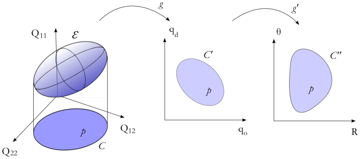
Figure 2: Schematic illustrating the transformation of probability regions at level $p$ due to variable transformations.

Lemma 4 (Parametric equation of probability regions).

For a SRF $X(\bm{\mathrm{s}})$ that satisfies the conditions of Lemma 2, the probability region of the anisotropy statistics corresponding to level $p\in[0,1]$ in $(R,\theta)$-space is given by the parametric equation

$$\left[y^{2}(\bm{\mathrm{q}};\bm{\mathrm{{Q}^{\ast}}},\bm{\mathrm{C}}_{\hat{\mathbb{Q}}})-\tilde{\lambda}_{1}(\bm{\mathrm{q}};\bm{\mathrm{{Q}^{\ast}}},\bm{\mathrm{C}}_{\hat{\mathbb{Q}}})\right]\,N=\ln(1-p),$$ (15)

where $y(\cdot)$, $\tilde{\lambda}_{1}(\cdot)$ are defined in (12) and $\bm{\mathrm{q}}\mapsto(R,\theta)$ by means of (4a) and (4b).

Proof.

The JPDF $f_{\hat{\mathbb{Q}}}$ is given by the trivariate Gaussian (9). Hence, the probability region of $\hat{\mathbb{Q}}$ is an ellipsoid whose surface satisfies the equation

$$({\mathbb{Q}}-\bm{\mathrm{{Q}^{\ast}}})^{t}\,\bm{\mathrm{C}}_{\hat{\mathbb{Q}}}^{-1}\,({\mathbb{Q}}-\bm{\mathrm{{Q}^{\ast}}})=\ell_{p},$$ (16)

where $\ell_{p}=F^{-1}(\chi^{2}=p,\nu=2)$ is the inverse of the chi-square cumulative distribution function with $\nu=2$ degrees of freedom (Siotani, 1964). Under the transformation ${\mathbb{Q}}\mapsto\bm{\mathrm{q}}$, the ellipsoid is projected onto an ellipse which is deformed by the transformation $\bm{\mathrm{q}}\mapsto(R,\theta)$ into an asymmetric convex curve (see Fig. 2). Based on (C-2), the equation of the corresponding ellipsoid in $(u,q_{\mathrm{d}},q_{\mathrm{o}})$-space is given by

$$z_{1}^{2}(\bm{\mathrm{q}};\bm{\mathrm{C}}_{\hat{\mathbb{Q}}})\,u^{2}+z_{2}(\bm{\mathrm{q}};\bm{\mathrm{{Q}^{\ast}}},{\bm{\mathrm{C}}_{\hat{\mathbb{Q}}}})\,u+\lambda_{1}(\bm{\mathrm{{Q}^{\ast}}},{\bm{\mathrm{C}}_{\hat{\mathbb{Q}}}})-\ell_{p}=0,$$

where the coefficients $z_{1}(\cdot),z_{2}(\cdot),\lambda_{1}(\cdot)$ are given by (11). The above quadratic equation has a unique real solution $u={Q}_{11}$ for any $\bm{\mathrm{q}}$ if the discriminant vanishes, i.e.,

$$z_{2}^{2}(\bm{\mathrm{q}};\bm{\mathrm{{Q}^{\ast}}},{\bm{\mathrm{C}}_{\hat{\mathbb{Q}}}})-4z_{1}^{2}(\bm{\mathrm{q}};\bm{\mathrm{C}}_{\hat{\mathbb{Q}}})\,\left[\lambda_{1}(\bm{\mathrm{{Q}^{\ast}}},{\bm{\mathrm{C}}_{\hat{\mathbb{Q}}}})-\ell_{p}\right]=0.$$ (17)

The equation above defines the probability region at level $p$. We can verify using (11) that (17) represents an ellipse in the space of $\bm{\mathrm{q}}$, i.e., it is equivalent to

$${\bm{\mathrm{q}}^{\prime}}^{t}\,\bm{\mathrm{M}}\,{\bm{\mathrm{q}}^{\prime}}=0,\,\text{where}$$

$$\bm{\mathrm{M}}=(\bm{\mathrm{C}}_{\hat{\mathbb{Q}}}^{-1}\,\bm{\mathrm{{Q}^{\ast}}})\,(\bm{\mathrm{C}}_{\hat{\mathbb{Q}}}^{-1}\,\bm{\mathrm{{Q}^{\ast}}})^{t}-(\bm{\mathrm{{Q}^{\ast}}}^{t}\,{\bm{\mathrm{C}}_{\hat{\mathbb{Q}}}^{-1}}\,\bm{\mathrm{{Q}^{\ast}}}-\ell_{p})\,{\bm{\mathrm{C}}_{\hat{\mathbb{Q}}}^{-1}}.$$

By inserting in (17) the functions $y$ and $\tilde{\lambda}_{1}$ used in (12) we obtain the parametric equation $2(\tilde{\lambda}_{1}-y^{2})\,N=\ell_{p}$, where by definition $F(\ell_{p},\nu=2)=p$. Since $F(x,\nu=2)=1-\exp(-x/2)$ (Abramowitz and Stegun, 1970, Eq. 26.4.1), it follows that $\ell_{p}=-2\ln(1-p)$, finally leading to (15). ∎

4 Non-parametric JPDF and Probability Region

The expressions for $f_{\hat{R},\hat{\theta}}(R,\theta;\bm{\mathrm{{Q}^{\ast}}},\bm{\mathrm{C}}_{\hat{\mathbb{Q}}})$ and the probability regions of $(\hat{R},\hat{\theta})$ above depend on the matrix $\bm{\mathrm{C}}_{\hat{\mathbb{Q}}}$, given by (1). $\bm{\mathrm{C}}_{\hat{\mathbb{Q}}}$ involves the series (1) that does not, in general, admit a closed form. If $H_{ij}(\bm{\mathrm{r}})$ decays fast for increasing $\|\bm{\mathrm{r}}\|$ we can use the explicit approximation $\bm{\mathrm{C}}_{\hat{\mathbb{Q}}}\approx\bm{\mathrm{C}}_{\hat{\mathbb{Q}}}^{(0)}$, where

$$\bm{\mathrm{C}}_{\hat{\mathbb{Q}}}^{(0)}=\frac{2}{N}\begin{bmatrix}{{Q}^{\ast}_{11}}^{2}&{{Q}^{\ast}_{12}}^{2}&{Q}^{\ast}_{11}\,{Q}^{\ast}_{12}\\ {{Q}^{\ast}_{12}}^{2}&{{Q}^{\ast}_{22}}^{2}&{Q}^{\ast}_{12}{Q}^{\ast}_{22}\\ {Q}^{\ast}_{11}{Q}^{\ast}_{12}&{Q}^{\ast}_{12}{Q}^{\ast}_{22}&\tfrac{1}{2}({{Q}^{\ast}_{12}}^{2}+{Q}^{\ast}_{11}{Q}^{\ast}_{22})\end{bmatrix}.$$ (18)

Figure 3 illustrates this fast decay of $C_{ij;kl}(\bm{\mathrm{r}})$ for isotropic (Fig. 3a) and anisotropic Gaussian covariance (Fig. 3b) functions.

(a) Isotropic: $\xi=1$, $\sigma^{2}=1$.

(b) Anisotropic: $\xi_{1}=1$, $\xi_{2}=2$, $\theta=30^{\circ}$, $\sigma^{2}=1$.

Figure 3: Plots of $C_{ij;kl}(\bm{\mathrm{r}})$ for (a) isotropic $(\xi=1)$ and (b) anisotropic ($\xi_{1}=1$, $\xi_{2}=2$ and $\theta=30^{\circ}$) Gaussian correlation functions. $C_{ij;kl}(\bm{\mathrm{r}})$ essentially vanishes outside a square of side $a\approx 2\xi$ (isotropic case) and $a\approx 3\max(\xi_{1},\xi_{2})$ (anisotropic case).

We expect that $\bm{\mathrm{C}}_{\hat{\mathbb{Q}}}^{(0)}$ will lead to a joint PDF with higher uncertainty, and hence more spread out than the true PDF, because it does not incorporate spatial correlations. We validated this intuitive argument by means of numerical simulations (see Section 6.1).

Theorem 4 (Non-parametric JPDF).

For an SRF $X(\bm{\mathrm{s}})$ that satisfies the conditions of Lemma 2, the non-parametric JPDF approximation $f^{(0)}_{\hat{R},\hat{\theta}}(R,\theta;\allowbreak{R}^{\ast},{\theta}^{\ast},N)$ of $(\hat{R},\hat{\theta})$ is given in the asymptotic regime by

$$f^{(0)}_{\hat{R},\hat{\theta}}(R,\theta;{R}^{\ast},{\theta}^{\ast},N) =\left\lvert\det(\bm{\mathrm{J}}_{\theta,R})\right\rvert f_{\hat{\bm{\mathrm{q}}}}^{(0)}(R,\theta;{R}^{\ast},{\theta}^{\ast},N),$$ (19a)

where

$$f_{\hat{\bm{\mathrm{q}}}}^{(0)}(R,\theta;{R}^{\ast},{\theta}^{\ast},N) \approx\frac{\sqrt{2\pi}\,\lambda_{2;0}}{z_{1;0}^{3}}\,\left(2y_{0}^{2}\,N+1\right)\,\mathrm{e}^{N\left(y_{0}^{2}-1/2\right)}.$$ (19b)

The coefficients $z_{1;0},y_{0},{\lambda}_{2;0}$ are given by the following expressions, where $\delta\theta=\theta-{\theta}^{\ast}$,

$$y_{0} =\frac{1}{\sqrt{2}\,z_{1;0}}\,\left[(R^{2}-1)({{R}^{\ast}}^{2}-1)\cos(2\delta\theta)-(R^{2}+1)({{R}^{\ast}}^{2}+1)\right],$$ (20a)

$$\lambda_{2;0} =\frac{\sqrt{2}\,({R}^{\ast})^{3}}{\pi^{3/2}}\,\left[(R^{2}+1)-(R^{2}-1)\cos(2\theta)\right]^{3},$$ (20b)

$${z}_{1;0}^{2} =(R^{2}-1)^{2}({{R}^{\ast}}^{2}-1)^{2}\cos(4\delta\theta)-4(R^{4}-1)({{R}^{\ast}}^{4}-1)\cos(2\delta\theta)$$ (20c)

$$+(R^{4}+1)(3{{R}^{\ast}}^{4}+2{{R}^{\ast}}^{2}+3)+2R^{2}({{R}^{\ast}}^{2}-1)^{2}.$$

Proof.

In (11) we replace $\bm{\mathrm{C}}_{\hat{\mathbb{Q}}}$ with $\bm{\mathrm{C}}_{\hat{\mathbb{Q}}}^{(0)}$, defined by (18). Thus, $z_{1},z_{2},\lambda_{1},\lambda_{2}$ are replaced, respectively, by $z_{1;0}$, $z_{2;0}$, $\lambda_{1;0}$, $\lambda_{2;0}$; then, $y_{0}=z_{2;0}/(2\sqrt{N}\,z_{1;0})$. Performing the calculations with $\bm{\mathrm{C}}_{\hat{\mathbb{Q}}}^{(0)}$ we obtain (20a)-(20c). The asymptotic result (13) of Lemma 3 is used in (19a) to obtain the non-parametric approximation (19b). Note that in the non-parametric approximation, the coefficient $\tilde{\lambda}_{1;0}$ in the exponent on the right hand side of (19b) is reduced to $1/2$. ∎

Numerical comparisons show that the absolute relative error between the non-parametric JPDF $f^{(0)}_{\hat{R},\hat{\theta}}(R,\theta;{R}^{\ast},{\theta}^{\ast},N)$ calculated with (i) the exact $f_{\bm{\mathrm{\hat{q}}}}^{(0)}(R,\theta;{R}^{\ast},{\theta}^{\ast},N)$, obtained from (12) by inserting the approximate covariance matrix $\bm{\mathrm{C}}_{\hat{\mathbb{Q}}}^{(0)}$, and (ii) the asymptotic limit given by (13), is less than $\approx 10^{-9}$ for $N=50$ and $\approx 10^{-6}$ for $N=30$.

Figure 4 demonstrates representative plots of the non-parametric JPDF based on (19). Note the bimodal structure of the JPDF for $N=100$ in Fig. 4a, with one mode at $R=1.2$ and the other (smaller) at $R\approx 0.8$. This is due to the considerable spread of $\hat{\theta}$, which results from the relatively small number of sampling points and the degeneracy of the anisotropy vector, i.e., the fact that the combination $(R,\theta)$ is equivalent to $(1/R,\theta-\pi/2)$; the degenerate peak at $(0.83,-70^{\circ})$ is folded into the primary domain. On the other hand, the smaller dispersion of $\hat{\theta}$ for $R=3$ leads to a single mode even for $N=100$.

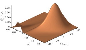
(a) ${R}^{\ast}=1.2$, ${\theta}^{\ast}=20^{\circ}$, $N=100$.

(b) ${R}^{\ast}=1.2$, ${\theta}^{\ast}=20^{\circ}$, $N=500$.

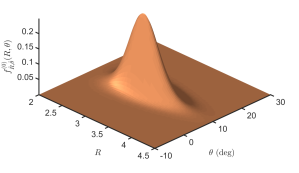
(c) ${R}^{\ast}=3$, ${\theta}^{\ast}=10^{\circ}$, $N=100$.

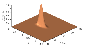
(d) ${R}^{\ast}=3$, ${\theta}^{\ast}=10^{\circ}$, $N=500$.

Figure 4: Non-parametric JPDF $f^{(0)}_{\hat{R},\hat{\theta}}(R,\theta)$ for various anisotropy parameters ${R}^{\ast},{\theta}^{\ast}$ and sample size $N$.

Knowledge of the anisotropy JPDF allows the construction of probability regions for the anisotropy statistics and confidence regions for the anisotropy parameters. For an SRF $X(\bm{\mathrm{s}})$ that satisfies the conditions of Lemma 2, the probability region corresponding to level $p$ of the anisotropy statistics (based on the simplifications of the non-parametric approximation), is given by the following slight modification of (15)

$$y_{0}^{2}(R,\theta;{R}^{\ast},{\theta}^{\ast})-\frac{1}{2}=\frac{\ln(1-p)}{N},$$ (21)

where $y_{0}$ is a function of the values $R,\theta$, and the parameters ${R}^{\ast},{\theta}^{\ast}$ as defined in (20a).

5 Statistical Test of Isotropy

Theorem 5 (Isotropic ratio).

Let $X(\bm{\mathrm{s}})$ be a statistically isotropic GSRF $({R}^{\ast}=1)$ which is sampled at $N$ points. Assume that the covariance $c({\bf r})$ is short-ranged and its spectral density satisfies $\tilde{C}({\bm{\mathrm{k}}})\sim\mathcal{O}(\|\bm{\mathrm{k}}\|^{-3-\epsilon})$ for $\epsilon>0$ as $\|\bm{\mathrm{k}}\|\rightarrow\infty$ as defined in Lemma 2. In addition, assume that the asymptotic regime conditions hold. The probability interval of the anisotropic ratio at probability level $p$ (for $N>2\ell_{p}$) is given by

$$\left(\frac{N-2\sqrt{\ell_{p}(N-\ell_{p})}}{N-2\ell_{p}},\frac{N+2\sqrt{\ell_{p}(N-\ell_{p})}}{N-2\ell_{p}}\right),$$ (22)

where $\ell_{p}=F^{-1}(\chi^{2}=p,\nu=2)=-2\ln(1-p)$ is the inverse of the chi square cumulative distribution function with two degrees of freedom.

Proof.

For ${R}^{\ast}=1$ the angle dependent terms in the equations (20) vanish, showing explicitly that the probability region is independent of $\theta$. Plugging (20a) in (21) the following quadratic in $R^{2}$ equation is obtained

$$N\,(R^{2}-1)^{2}-2\ell_{p}\,(R^{4}+1)=0.$$

In fact, the probability region is reduced to a one-dimensional probability interval whose endpoints coincide with the roots of the above equation. The constraint $N>2\ell_{p}$ is in practice satisfied for $N\to\infty$ and ensures that the roots of the above equation are positive real numbers. Based on the definition of $\ell_{p}$ the constraint is equivalent to $N>-4\ln(1-p)$. For example, $p=0.95$ implies $\ell_{p}\approx 6$ and $N>12$. ∎

Equation (22) is independent of $c(\bm{\mathrm{r}})$ and thus provides a non-parametric approximation of the probability interval for ${R}^{\ast}$. The JPDF (19) is independent of $\theta$ and ${\theta}^{\ast}$ for ${R}^{\ast}=1$. The PDF, $f_{\hat{R}}^{(0)}(R)$, of $\hat{R}$ for ${R}^{\ast}=1$ and $N=100$ is shown in Fig. 5, including the $95\%$ probability interval predicted by (22).

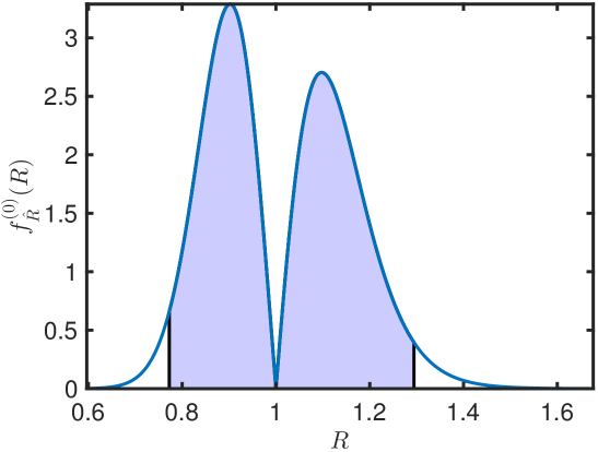
Figure 5: Non-parametric sampling PDF of the anisotropic ratio, $f_{\hat{R}}^{(0)}(R)$, for an isotropic random field sampled at $N=100$ points. Shaded area represents the corresponding $95\%$ probability interval $(R_{-},R_{+})=(0.77,1.29)$.

Note that the PDF has a node instead of a peak at $R=1$. This is not an artifact of the non-parametric approximation, since the complete JPDF (14) also vanishes at $R=1$. The node is due to the root of the Jacobian (D-1) at $R=1$, which reflects that the isotropic point $(1,0)$ in $(q_{\mathrm{d}},q_{\mathrm{o}})$-space is mapped onto the straight line $R=1$ in the $(R,\theta)$-space. The node is also evident in numerical simulations that do not use the Jacobian (see Figure 7 below).

6 Application to Simulated and Real Data

To apply the formalism developed above to data sets that comprise discrete sets of values, we replace the partial derivatives by respective discrete operators $\check{\partial}{X}_{i}(\bm{\mathrm{s}}_{k})$, $i=1,2$. The respective estimates of $\bm{\mathrm{{Q}^{\ast}}}$ are denoted by $\bm{\mathrm{\check{Q}}}$. The discretization introduces a bias that increases with the sparsity of the sampling pattern. A “good” sampling pattern is characterized by a typical distance $\hat{a}$ between nearest neighbors which is approximately uniform (ideally, a regular lattice pattern is best) and $\hat{a}\ll\min(\xi_{1},\xi_{2})$, where $\xi_{1},\xi_{2}$ are the principal correlation lengths. Different approaches for estimating $\check{\partial}{X}_{i}(\bm{\mathrm{s}}_{k})$ are investigated in (Chorti and Hristopulos, 2008). Herein, the centered differences scheme is used for gridded data.

We denote average values of a statistic over different samples (repetitions) by a bar over the respective symbol, i.e., $\overline{\check{Q}}_{ij}$. For simulated data, the ensemble properties $\bm{\mathrm{{Q}^{\ast}}}$ and $\bm{\mathrm{C}}_{\hat{\mathbb{Q}}}$ which are unknown a priori, are replaced by the respective averages $\bm{\mathrm{{Q}^{\ast}}}\approx(\overline{\check{Q}}_{11},\overline{\check{Q}}_{22},\overline{\check{Q}}_{12})^{t}$ and ${\bm{\mathrm{C}}_{\hat{\mathbb{Q}}}}\approx\bm{\mathrm{C}}_{\bm{\mathrm{\overline{\check{Q}}}}}$. In the non-parametric approximation, $\bm{\mathrm{C}}_{\hat{\mathbb{Q}}}^{(0)}$ is obtained from (18) by replacing $\bm{\mathrm{{Q}^{\ast}}}$ with $\overline{\bm{\mathrm{\check{Q}}}}$.

6.1 Simulated Scattered Data

We generate SRF realizations with specified $({R}^{\ast},{\theta}^{\ast})$ to validate the probability region of the anisotropy parameters (21). Figure 6 and Table 1 investigate the anisotropic case ${R}^{\ast}=1.5$, ${\theta}^{\ast}=-30^{\circ}$, whereas the isotropic case is considered in Table 2 and Figure 7. A desktop computer with an Intel^® Core^™ i5-2500 (4 cores, 3.30 GHz) CPU running Matlab^® R2015b under 64-bit Windows^® 7, was used for all the simulations.

We simulate scattered data using the following method: First, a realization of an GSRF is generated on a regular grid. The Fourier Filtering Method (Pardo-Igúzquiza and Chica-Olmo, 1993; Lantuéjoul, 2002; Hristopulos, 2005) is used on $L\times L$ square grids with lattice constant $a=1$. We use Gaussian, $c(\bm{\mathrm{r}})=\sigma^{2}\,\exp(-\|\bm{\mathrm{r}}\|^{2}/\xi^{2})$, and Matérn, $c(\bm{\mathrm{r}})=\sigma^{2}\,2^{1-\nu}\,\Gamma(\nu)^{-1}\,\xi^{-\nu}\times\allowbreak\|\bm{\mathrm{r}}\|^{\nu}K_{\nu}(\|\bm{\mathrm{r}}\|/\xi)$, covariance functions (expressions correspond to the isotropic case), where $\Gamma(\cdot)$ is the Gamma and $K_{\nu}(\cdot)$ the modified Bessel function of order $\nu$. In the Gaussian case, the correlation range is controlled by $\xi$ whereas in the Matérn case by both $\xi$ and $\nu$. The smoothness parameter $\nu$ adjusts the differentiability of the SRF: $\nu=1/2$ corresponds to the non-differentiable exponential function and $\nu\to\infty$ to the infinitely differentiable Gaussian. For given $\xi$, the field is smoother for higher $\nu$. To compensate for this effect and to compare SRFs of similar spatial variability, we use rescaled correlation lengths $\tilde{\xi}=A_{d}\xi$, where $A_{d}$ is the integral scale factor (Hristopulos and Žukovič, 2011): In $d=2$, $A_{d}=2\sqrt{\pi\nu}$ for Matérn correlations whereas for Gaussian correlations $A_{d}=\sqrt{\pi}$. For equal rescaled correlation lengths, $\tilde{\xi}_{\text{Gauss}}=\tilde{\xi}_{\text{Mat\'{e}rn}}$, with $d=2$, $\nu=2$, it follows that $\xi_{\text{Gauss}}=2\sqrt{2}\,\xi_{\text{Mat\'{e}rn}}$.

We randomly choose a fraction of the grid points to mimic scattered data. For a square lattice of side $L$ a sample of $N=(\rho L)^{2}$ points are randomly chosen from Gaussian and Matérn lattice SRFs. An estimate of the mean distance between $N$ uniformly distributed points is $L/\sqrt{N}=1/\rho$, thus $\rho$ is the mean sampling frequency. The samples respect the condition that the correlation lengths exceed the mean distance between the points, as specified in the first paragraph of this Section.

We employ the natural neighbor interpolation method (Fisher et al., 2005) in Matlab^® on an $M\times M$ square grid with $M=200$. Natural neighbor interpolation provides smooth surfaces and does not assume isotropy of the data; however, it is defined only inside the convex hull of the data sites. Due to the occasionally poor sampling near the domain boundaries, interpolation artifacts appear (Bobach et al., 2009) as elongated islands, oriented vertically along the left and horizontally along the bottom sides of the domain. Hence, they tend to bias the anisotropy estimates towards higher or lower anisotropy ratios and angles near zero. Thus, boundary strips of thickness $L/\sqrt{N}$ are discarded from the interpolation surface to minimize bias. The partial derivatives are estimated via centered differences on the interpolated surface. Finally, we perform anisotropy estimation for each sample and compute the non-parametric probability region at $p=0.95$ using ensemble averages. Also, we compute confidence regions for each anisotropy estimate at several confidence levels.

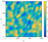
(a) Gaussian SRF, ${R}^{\ast}=1.5$, ${\theta}^{\ast}=-30^{\circ}$

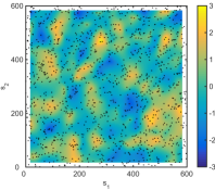
(b) 1296 random nodes and interpolated field.

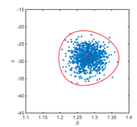
(c) Anisotropy estimates and probability region

(d) Matérn SRF, ${R}^{\ast}=1.5$, ${\theta}^{\ast}=-30^{\circ}$

(e) 1296 random nodes and interpolated field.

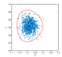
(f) Anisotropy estimates and probability region

Figure 6: Non-parametric probability region estimation for scattered data. (a) and (d): Realization of zero-mean, unit-variance anisotropic Gaussian SRF with $\xi=28.3$ and Mátern SRF with $\nu=2$ and $\xi=10$ on a $600\times 600$ square grid. (b) and (e): Random sample of $N=1296$ points and interpolated field on a $200\times 200$ grid using natural neighbors. Boundary strips of thickness $L/\sqrt{N}$ were discarded from the interpolated field to avoid interpolation artifacts at the domain boundary. (c) and (f): Anisotropy estimates (crosses) are generated from $1000$ random samples of $N=1296$ points; the continuous curve corresponds to $95\%$ non-parametric probability region calculated with the ensemble-based anisotropy estimates $(\overline{\check{R}},\ \overline{\check{\theta}})$, which are denoted by a small circle inside the cloud.

6.1.1 Anisotropic Scattered Data

Figure 6a demonstrates a realization of a zero-mean, unit variance anisotropic GSRF with Gaussian covariance with ${R}^{\ast}=1.5,{\theta}^{\ast}=-30^{\circ}$, $\xi=28.3$ on a $600\times 600$ grid. A randomly extracted set of $N=1296$ points ($\rho=0.06$) is shown in Fig. 6b. The depicted smooth field is generated from the 1296 points by interpolation and is used to estimate $(\check{R},\check{\theta})$.

In Figure 6c the non-parametric probability region (red contour) at $p=0.95$, defined by (21) is compared with CHI anisotropy estimates (blue crosses) from $1000$ SRF samples. For each sample, we estimate $\bm{\mathrm{{Q}^{\ast}}}$ by means of the spatial average $\bm{\mathrm{\check{Q}}}$ and then calculate $(\check{R},\check{\theta})$ by applying (5). We estimate $({R}^{\ast},{\theta}^{\ast})$ based on the $\overline{\check{R}},\ \overline{\check{\theta}}$, which are obtained from the ensemble average $\overline{\bm{\mathrm{\check{Q}}}}$ by means of Theorem 2. The ensemble-based anisotropy estimate $(\overline{\check{R}},\ \overline{\check{\theta}})$, is denoted by a small circle inside the cloud of the $(\check{R},\check{\theta})$ points. Figures 6d–6f demonstrate the simulated scattered data probability region estimation for a zero-mean, unit-variance Matérn covariance with ${R}^{\ast}=1.5,{\theta}^{\ast}=-30^{\circ}$, $\xi=10$, $\nu=2$. The normality of $\hat{\mathbb{Q}}$, supported by CLT considerations as shown in Lemma 2, was confirmed by normal probability plots (not shown here).

The non-parametric probability region (Theorem 4) extends beyond the region obtained from the true JPDF (this is supported by Figures 6c and 6f as explained below). We conducted numerical experiments (not shown here) for several values of $\tilde{\xi}/a$ and $N$ to confirm that non-parametric probability regions based on (19a) are more extended in parameter space than the regions based on the true JPDF (12). If $\tilde{\xi}/a\to 0$, i.e., as the spatial extent of the correlations is reduced, the scatter cloud of $(\check{R},\check{\theta})$ expands and tends to fill the non-parametric probability region. On the other hand, as $\tilde{\xi}/a$ increases, i.e., for dense sampling of the SRF, the scatter cloud tends to be confined inside the smaller parametric region. These observations agree with our earlier statement that the non-parametric approximation contains the true probability region.

In Table 1 we validate the non-parametric anisotropy confidence region for simulated scattered Gaussian ($\xi=28.3$) and Matérn ($\xi=10$, $\nu=2$) covariance functions with ${R}^{\ast}=1.5$ and ${\theta}^{\ast}=-30^{\circ}$. We generate 1000 realizations for different domain sizes ($L=600$, $800$, $1000$, $1200$) and mean sampling frequencies ($\rho=0.04,0.06$) and we enumerate the number of simulations for which the ensemble means $\overline{\check{R}},\overline{\check{\theta}}$ (as estimates of the population means) are outside the non-parametric confidence region. The latter is computed for each anisotropy estimate at different confidence levels ($p=0.95$, $0.75$, $0.68$, $0.5$, $0.25$) using (21). If the true JPDF and the confidence regions of the anisotropy statistics are known at the $p$ levels above, the average number of simulations for which the true confidence region does not contain the ensemble means $\overline{\check{R}},\overline{\check{\theta}}$ is $50$, $250$, $320$, $500$, and $750$ respectively. However, the number of simulations for which $\overline{\check{R}},\overline{\check{\theta}}$ lie outside the non-parametric region (21) is always less than expected for the true confidence regions. This observation agrees with the proposition that the non-parametric confidence region (21) contains the true confidence region.

Table 1: Numerical validation of the non-parametric anisotropy confidence region for simulated scattered data. Anisotropy estimates were computed from 1000 random samples of $N$ points from (a) Gaussian and (b) Matérn lattice SRFs with $R=1.5$, $\theta=-30^{\circ}$. For each lattice size $L$ and sampling frequency $\rho$, $N_{\text{out},p}$ is the number of anisotropy estimates for which the non-parametric confidence region computed at $p=0.95$, $0.75$, $0.68$, $0.5$, and $0.25$ using Theorem 4, does not contain the ensemble mean $(\overline{\check{R}},\overline{\check{\theta}})$.

$L$	$600$		$800$		$1000$		$1200$
$N$	$576$	$1296$	$1024$	$2304$	$1600$	$3600$	$2304$	$5184$
$N_{\text{out},p=0.95}$	$12$	$3$	$10$	$3$	$1$	$0$	$6$	$1$
$N_{\text{out},p=0.75}$	$132$	$68$	$106$	$41$	$83$	$26$	$85$	$20$
$N_{\text{out},p=0.68}$	$194$	$102$	$159$	$68$	$141$	$48$	$128$	$47$
$N_{\text{out},p=0.50}$	$380$	$280$	$324$	$191$	$288$	$155$	$274$	$166$
$N_{\text{out},p=0.25}$	$658$	$560$	$601$	$534$	$592$	$465$	$574$	$450$
$\overline{\check{R}},\overline{\check{\theta}}$	$1.19,-29.0^{\circ}$	$1.28,-29.8^{\circ}$	$1.21,-29.8^{\circ}$	$1.30,-29.7^{\circ}$	$1.22,-30.1^{\circ}$	$1.31,-30.1^{\circ}$	$1.22,-30.4^{\circ}$	$1.32,-30.9^{\circ}$

(a) Gaussian, $R=1.5$, $\theta=-30^{\circ}$, $\xi=28.3$, $\rho=0.04,0.06$

$L$	$600$		$800$		$1000$		$1200$
$N$	$576$	$1296$	$1024$	$2304$	$1600$	$3600$	$2304$	$5184$
$N_{\text{out},p=0.95}$	$8$	$4$	$10$	$3$	$5$	$2$	$11$	$4$
$N_{\text{out},p=0.75}$	$150$	$78$	$130$	$69$	$95$	$42$	$114$	$51$
$N_{\text{out},p=0.68}$	$209$	$121$	$172$	$120$	$138$	$78$	$170$	$86$
$N_{\text{out},p=0.50}$	$391$	$289$	$346$	$257$	$302$	$206$	$320$	$227$
$N_{\text{out},p=0.25}$	$680$	$608$	$667$	$572$	$632$	$515$	$630$	$543$
$\overline{\check{R}},\overline{\check{\theta}}$	$1.14,-28.1^{\circ}$	$1.22,-28.9^{\circ}$	$1.16,-29.5^{\circ}$	$1.23,-29.8^{\circ}$	$1.16,-30.0^{\circ}$	$1.24,-30.3^{\circ}$	$1.17,-30.4^{\circ}$	$1.25,-30.7^{\circ}$

(b) Matérn, $R=1.5$, $\theta=-30^{\circ}$, $\nu=2$, $\xi=10$,$\rho=0.04,0.06$

6.1.2 Isotropic Scattered Data

We numerically validate the isotropy testing procedure by enumerating the number of anisotropy estimates that fall outside the probability region at $p=0.95$ for 1000 realizations of simulated scattered data in different domain sizes ($L=600,800,1000,1200$), mean sampling frequency ($\rho=0.04,0.06$), and isotropic covariances (Gaussian with $\xi=28.3$, Matérn with $\xi=10,\nu=2$). If the true JPDF and the probability regions of the anisotropy statistics are known at $p=0.95$ probability level, on average 50 out of the 1000 simulations should fall outside the true region. In Table 2, $N_{\text{out,iso}}$ is the number of estimates that fall outside the $p=0.95$ isotropy probability interval $(R_{-},R_{+})$ using Eq. (22) while $N_{\text{out}}$ is the number of samples that fall outside the probability region calculated using the ensemble-based anisotropy estimate $(\overline{\check{R}},\ \overline{\check{\theta}})$ and Theorem 4. The mean time $\bar{t}$ for anisotropy estimation per processor core is also shown with an error estimate of one standard deviation.

Table 2: Numerical validation of the non-parametric isotropy test at $p=0.95$ for simulated scattered data. Anisotropy estimates generated from 1000 random samples of $N$ points from isotropic (a) Gaussian and (b) Matérn lattice SRFs. For each lattice size $L$ and sampling frequency $\rho$, $N_{\text{out,iso}}$ is the number of simulations that fall outside the non-parametric probability region estimated from $\overline{\bm{\mathrm{\check{Q}}}}$ using Theorem 4. $N_{\text{out}}$ is the number of simulations that fall outside the non-parametric isotropy interval $(R_{-},R_{+})$ based on (22). $\bar{t}$: average time per anisotropy estimation (per processor core) with an error estimate of one standard deviation.

$L$	$600$		$800$		$1000$		$1200$
$N$	$576$	$1296$	$1024$	$2304$	$1600$	$3600$	$2304$	$5184$
$N_{\text{out,iso}}$	$14$	$4$	$12$	$2$	$6$	$0$	$11$	$1$
$N_{\text{out}}$	$12$	$3$	$13$	$2$	$5$	$0$	$9$	$1$
$\overline{\check{R}},\overline{\check{\theta}}$	$0.990,-42.2$	$0.986,-43.2$	$0.995,-41.6$	$0.992,-42.2$	$0.997,-43.0$	$1.00,41.8$	$0.998,-42.5$	$1.00,44.9$
$R_{-},R_{+}$	$0.902,1.11$	$0.934,1.07$	$0.926,1.08$	$0.950,1.05$	$0.940,1.06$	$0.960,1.04$	$0.950,1.05$	$0.967,1.03$
$\bar{t}$ (msec)	$129\pm 4$	$131\pm 3$	$132\pm 3$	$146\pm 5$	$141\pm 5$	$160\pm 5$	$150\pm 9$	$175\pm 6$

(a) Gaussian, $\xi=28.3$, $\rho=0.04,0.06$

$L$	$600$		$800$		$1000$		$1200$
$N$	$576$	$1296$	$1024$	$2304$	$1600$	$3600$	$2304$	$5184$
$N_{\text{out,iso}}$	$15$	$8$	$12$	$8$	$10$	$5$	$10$	$7$
$N_{\text{out}}$	$11$	$7$	$12$	$5$	$10$	$2$	$12$	$4$
$\overline{\check{R}},\overline{\check{\theta}}$	$0.990,-44.4$	$1.01,43.6$	$1.01,42.7$	$0.993,-42.3$	$1.00,43.6$	$1.01,44.2$	$0.997,-37.6$	$1.00,42.8$
$R_{-},R_{+}$	$0.902,1.11$	$0.934,1.07$	$0.926,1.08$	$0.950,1.05$	$0.940,1.06$	$0.960,1.04$	$0.950,1.05$	$0.967,1.03$
$\bar{t}$ (msec)	$129\pm 3$	$131\pm 4$	$130\pm 4$	$143\pm 5$	$139\pm 6$	$156\pm 5$	$145\pm 5$	$169\pm 7$

(b) Matérn, $\nu=2$, $\xi=10$, $\rho=0.04,0.06$

Figure 7 demonstrates the non-parametric probability regions and the scatter cloud of anisotropy estimates for scattered data sampled from isotropic Gaussian and Matérn lattice SRFs of increasing side $L$. The absence of estimates near the $R=1$ line agrees with the existence of a JPDF node at $R=1$ as discussed in Section 5. For smaller domains the anisotropy estimates deviate from isotropy.

The computational complexity of natural neighbors interpolation is $\mathcal{O}((M+N)\log N)$ (Park et al., 2006), where $M$ is the number of the interpolation points. The complexity of derivative estimation using centered differences is $\mathcal{O}(M)$. Hence, $\mathcal{O}(2M)$ operations are needed for computing $\check{\partial_{i}}X(\bm{\mathrm{s}})$, $i=1,2$ and $\mathcal{O}(3M)$ operations for $\hat{Q}_{ij}$. Thus the total computation time $t_{M,N}$ is of $\mathcal{O}(5M+(M+N)\log N)$, from which we obtain $t_{M^{\prime},N^{\prime}}/t_{M,N}=(5M^{\prime}+(M^{\prime}+N^{\prime})\log N^{\prime})/(5M+(M+N)\log N)$. For $M=200^{2}$, $t_{N=5184}/t_{N=576}=1.28$. The time ratio obtained from Table 2a is $\bar{t}_{N=5184}/\bar{t}_{N=576}=1.36\pm 0.06$ and from Table 2b is $\bar{t}_{N=5184}/\bar{t}_{N=576}=1.31\pm 0.06$. For $M=100^{2}$, $t_{N=5184}/t_{N=576}=1.53$ while the simulation times (average times per anisotropy estimation per processor core) obtained for 1000 realizations of isotropic Matérn covariance (not shown here) are $\bar{t}_{N=576}=36.4\pm 1.5\text{ msec}$ and $\bar{t}_{N=5184}=58.3\pm 2.6\text{ msec}$, giving $\bar{t}_{N=5184}/\bar{t}_{N=576}=1.60\pm 0.10$.

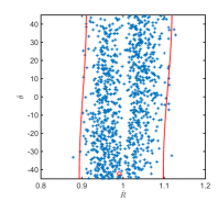
(a) Gaussian, $L=600$, $N=576$

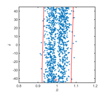
(b) Gaussian, $L=800$, $N=1024$

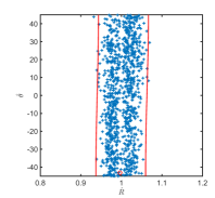
(c) Gaussian, $L=1000$, $N=1600$

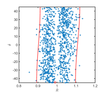
(d) Matérn, $L=600$, $N=576$

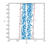
(e) Matérn, $L=800$, $N=1024$

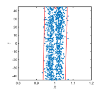
(f) Matérn, $L=1000$, $N=1600$

Figure 7: Non-parametric probability region estimation for isotropic scattered data. The initial lattice SRF is defined over a square lattice with side $L=600,800,1000$. The continuous curve corresponds to $95\%$ non-parametric probability region calculated with anisotropy parameters estimated from $\overline{\bm{\mathrm{\check{Q}}}}$. (a)–(c) Anisotropy estimates (crosses) generated from $1000$ random samples obtained from a zero-mean, unit-variance isotropic Gaussian SRF with $\xi=28.3$. (d)–(f) Anisotropy estimates (crosses) generated from $1000$ random scattered samples obtained from a zero-mean, unit-variance Matérn SRF with $\xi=10$.

6.2 Case Study: Radiation Exposure

We study anisotropy in two data sets of daily averages of radioactivity gamma dose rates over part of the Federal Republic of Germany, which was provided by the German automatic radioactivity monitoring network for the Spatial Interpolation Comparison (SIC 2004) exercise (Dubois and Galmarini, 2006). Dose rates are measured in nanosieverts per hour (nSv/h). The background data set corresponds to typical radioactivity measurements ($\approx 100$ nSv/h), which follow the Gaussian distribution (graph not shown), and thus their skewness and excess kurtosis coefficients are close to zero. The emergency data includes a simulated local release of radioactivity which results in five dose rate “measurements” around $10$ times above background (exceeding $1000$ nSv/h). These measurements are aligned in the East-West direction. Table 3 summarizes the statistics of both data sets. The two rightmost columns show the CHI-based estimates of anisotropy parameters.

Table 3: Summary statistics of radioactivity dose rate exhaustive data sets (units are in nanosieverts per hour) and CHI anisotropy estimates. Abbreviations: min: minimum sample value; med: median sample value, max: maximum sample value; std: sample standard deviation; skew: sample skewness coefficient; kurt: sample excess kurtosis coefficient; $\check{R},\,\check{\theta}$: estimates of anisotropy parameters.

$N=1008$	min	mean	med	max	std	skew	kurt	$\check{R}$	$\check{\theta}$
Background	57.0	97.7	98.6	180.0	19.6	0.4	0.6	1.18	$7.36^{\circ}$
Emergency	57.0	106.1	98.9	1528.2	92.5	11.3	144.1	0.45	$-0.75^{\circ}$

Since the 95% confidence interval for isotropy is $(R_{-},R_{+})=(0.92,1.08)$, this dataset can be considered as slightly anisotropic. The direction of anisotropy is different in the two sets: In the background set the axis $A_{1}$ is tilted with respect to the x-axis (which is aligned with the E-W direction) by $7.36^{\circ}$, while the dominant anisotropy axis is $A_{2}$ since $\xi_{2}=1.18\xi_{1}$. $A_{2}$ is closer to the y-axis, implying a dominant North-South anisotropy. In the emergency set the axis $A_{1}$ is slightly tilted with respect to the x-axis (by $-0.75^{\circ}$), and the dominant anisotropy axis is $A_{1}$ since $\xi_{2}=0.45\xi_{1}$. Since $A_{1}$ is closer to the x-axis, this implies that the radioactive plume reverses the dominant anisotropy direction to East-West.

We calculate the non-parametric JPDF and the 95% confidence regions of the anisotropy statistics based on the estimated anisotropy parameters (i.e., by CHI anisotropy estimation on gridded values obtained by natural neighbor interpolation) for both sets. The results are shown in Fig. 8.

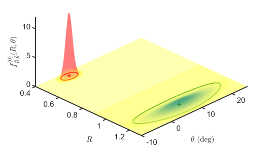
Figure 8: Non-parametric joint PDF shaded surfaces (red and green online) and 95% confidence regions (solid contours) for the radioactivity dose rate data sets: background measurements (right) and emergency data simulation (left).

There is no overlap of the two joint density functions, and the contours corresponding to the 95% confidence regions do not intersect. These patterns suggest statistically significant anisotropy difference between the background and the emergency data due to the elevated values of the dose rate in the East-West direction of the spreading plume which changes the orientation of the major anisotropy axis.

7 Discussion and Conclusions

This work focuses on the estimation of geometric anisotropy in scattered or grid-based two-dimensional data. We derive explicit expressions for the joint PDF of the anisotropy statistics, given by equations (13)-(14), and for the corresponding anisotropy probability regions at any level, i.e., equation (15). The main assumptions used are that (i) the data are drawn from a jointly Gaussian, stationary and differentiable random field and (ii) the covariance function is short-ranged.

We also derive a non-parametric approximation for the joint PDF of the anisotropy statistics, which can be used if the covariance function is unknown a priori, or if estimation of the covariance is not desired. The non-parametric approximation of the anisotropy joint PDF is given by (19). The corresponding equation for the non-parametric approximation of the probability region is given by (21). We also derive probability intervals for the anisotropy ratio under the hypothesis that the sample comes from an isotropic random field. These probability intervals are used to formulate a non-parametric test of the isotropic hypothesis. We illustrate the application of the joint PDF and the probability regions with simulated and real data.

The Gaussian assumption is used in the decomposition of the covariance matrices $\bm{\mathrm{C}}_{\hat{\mathbb{Q}}}$ and $\bm{\mathrm{C}}_{\hat{\mathbb{Q}}}^{(0)}$, i.e., to derive equations (1) and (18) by means of the Wick-Isserlis theorem. This decomposition can be justified in principle, albeit approximately, even for non-Gaussian densities, based on optimal variational (Gaussian) approximations. Practical application of the derived formulas requires the estimation of anisotropy statistics using CHI. Accurate estimation based on CHI requires in addition to (i) and (ii) above the following: (iii) a large sample size, $N\to\infty$ and (iv) a sample domain that is large with respect to the correlation area. The latter is difficult to satisfy in case of large anisotropy $({R}^{\ast}\gg 1$ or ${R}^{\ast}\ll 1)$. In such cases, the CHI estimate tends to underestimate the actual anisotropy. CHI anisotropy estimates include biases due to (v) the finite step size of the grid and (vi) interpolation (in the case of scattered data).

In summary, our approach consists of the following steps: (i) If necessary, preprocess the data in order to remove trends and use transforms to reduce deviations from the Gaussian distribution (e.g., Box-Cox transform). (ii) Choose an interpolator which provides smooth interpolation surfaces. Several interpolators were tested and compared in (Chorti and Hristopulos, 2008). The interpolation grid should be dense to allow accurate approximation of the spatial derivatives. (iii) Compute the partial derivatives of the interpolated surface. (iv) Compute $\hat{Q}_{ij}$ and use Theorem 2 to obtain anisotropy parameter estimates. (v) The non-parametric JPDF is obtained from Theorem 4. The probability regions are provided by Lemma 4 using the approximate non-parametric covariance matrix, i.e. (18). (vi) The isotropy test of Theorem 5 can be used to test for the presence of anisotropy. (vii) The differentiability assumption can be tested a posteriori by determining the optimal anisotropic variogram model using standard geostatistical procedures. In this step, the CHI anisotropy estimates can be used to fix the anisotropy parameters or to provide informed initial guesses for likelihood optimization.

Our approach provides a computationally efficient, albeit approximate, method of geometric anisotropy estimation in two dimensions, because the analytical expressions derived above can be evaluated with minimal computational cost. The most computationally intensive part is the interpolation of scattered data onto regular grids in order to calculate derivatives. We use natural neighbor interpolation which is computationally fast (its complexity is essentially determined by Voronoi tesselation). For small datasets, the computation time scales linearly with the number of nodes $M$ of the interpolation grid, while for large datasets the computational cost is dominated by $\mathcal{O}(M\log N)$ where $N$ is the number of data points. A formulation of the natural neighbor interpolation algorithm which directly provides the partial derivatives of the interpolated surface is also available (Sambridge et al., 1995, Appendix A1).

Our approach could be useful in estimating anisotropy in big data sets. In addition, the non-parametric JPDF can be used as an anisotropy prior in Bayesian and copula analyses (Kazianka, 2013). The method also provides initial estimates for maximum likelihood estimation of spatial anisotropic models (Pebesma et al., 2011). Furthermore, it furnishes an easily computable indicator of physical change in spatially extended systems based on the comparison of anisotropy probability regions.

Straightforward extension of this work is possible for the joint lognormal distribution along the lines of (Chorti and Hristopulos, 2008). The global statistical measures of anisotropy can be efficiently calculated for large domains and can thus provide a useful statistic for large data sets. Local variations of anisotropy can also be investigated using windowing methods. Capturing such local variability has applications in the analysis of medical images, e.g. (Richard and Bierme, 2010). Currently, the solution of the non-linear CHI equations for $d>2$ is not available in closed form. Hence, an analytical expression of the anisotropy joint PDF in higher than two dimensions is not yet feasible. Another path for future research is the development of an anisotropy detection method which will involve local integrals of the field values. Such an approach, if analytically tractable, will apply to non-differentiable random fields as well.

Appendix A: Proof of Lemma 1

Proof.

Using the definition (7) we obtain

$$C_{ij;kl} =\operatorname{Cov}\left(\frac{1}{N}\sum_{n=1}^{N}{X}_{ij}(\bm{\mathrm{s}}_{n}),\frac{1}{N}\sum_{m=1}^{N}{X}_{kl}(\bm{\mathrm{s}}_{m})\right)$$

$$=\frac{1}{N^{2}}\sum_{n,m}\operatorname{Cov}\left({X}_{ij}(\bm{\mathrm{s}}_{n}),{X}_{kl}(\bm{\mathrm{s}}_{m})\right).$$ (A-1)

Due to the stationarity of $X(\bm{\mathrm{s}})$, the double series in (Proof.) is reduced to a single series over all $(N^{2})$ lag vectors $\bm{\mathrm{r}}_{nm}=\bm{\mathrm{s}}_{n}-\bm{\mathrm{s}}_{m}$ $(n,m=1,\ldots,N)$, i.e.,

$$C_{ij;kl} =\frac{1}{N^{2}}\sum_{\bm{\mathrm{r}}_{nm}}\operatorname{Cov}\left(X_{ij}(\bm{\mathrm{s}}_{0}),X_{kl}(\bm{\mathrm{s}}_{0}+\bm{\mathrm{r}}_{nm})\right)$$

$$=\frac{1}{N}\operatorname{Cov}\left(X_{ij}(\bm{\mathrm{0}}),X_{kl}(\bm{\mathrm{0}})\right)+\frac{1}{N^{2}}\sum_{\bm{\mathrm{r}}_{nm}\neq\bm{\mathrm{0}}}\operatorname{Cov}\left(X_{ij}(\bm{\mathrm{0}}),X_{kl}(\bm{\mathrm{r}}_{nm})\right).$$ (A-2)

Covariance of the gradient tensor: Let $\bm{\mathrm{r}}$ denote any lag vector (including $\bm{\mathrm{r}}=\bm{\mathrm{0}}$) between two points. Based on the definition of the covariance function it follows that

$$\operatorname{Cov}\left(X_{ij}(\bm{\mathrm{0}}),X_{kl}(\bm{\mathrm{r}})\right)={\mathbb{E}}\left[X_{ij}(\bm{\mathrm{0}})X_{kl}(\bm{\mathrm{r}})\right]-{\mathbb{E}}\left[X_{ij}(\bm{\mathrm{0}})\right]{\mathbb{E}}\left[X_{kl}(\bm{\mathrm{r}})\right].$$ (A-3)

Note that

$${\mathbb{E}}\left[X_{ij}(\bm{\mathrm{0}})X_{kl}(\bm{\mathrm{r}})\right]={\mathbb{E}}\left[\partial_{i}{X}(\bm{\mathrm{0}})\,\partial_{j}{X}(\bm{\mathrm{0}})\,\partial_{k}{X}(\bm{\mathrm{r}})\,\partial_{l}{X}(\bm{\mathrm{r}})\right].$$

For a differentiable and stationary SRF $X(\bm{\mathrm{s}})$, the gradient component ${\partial}_{i}{X}(\bm{\mathrm{s}})$ is a zero-mean Gaussian SRF with covariance function given by (Abrahamsen, 1997; Yaglom, 1987)

$${\mathbb{E}}\left[\partial_{i}{X}(\bm{\mathrm{s}})\,\partial_{j}{X}(\bm{\mathrm{s}}+{\bf r})\right]=-\frac{\partial^{2}c(\bm{\mathrm{r}})}{\partial r_{i}\partial r_{j}}.$$ (A-4)

Hence, ${\mathbb{E}}\left[X_{ij}(\bm{\mathrm{0}})\,X_{kl}(\bm{\mathrm{r}})\right]$ can be calculated using the moment factorization property of multivariate normal distributions (Isserlis, 1918; Wick, 1950)

$${\mathbb{E}}\left[X_{ij}(\bm{\mathrm{0}})X_{kl}(\bm{\mathrm{r}})\right] ={\mathbb{E}}\left[\partial_{i}{X}(\bm{\mathrm{0}})\partial_{j}{X}(\bm{\mathrm{0}})\right]{\mathbb{E}}\left[\partial_{k}{X}(\bm{\mathrm{r}})\partial_{l}{X}(\bm{\mathrm{r}})\right]$$

$$+{\mathbb{E}}\left[\partial_{i}{X}(\bm{\mathrm{0}})\partial_{k}{X}(\bm{\mathrm{r}})\right]{\mathbb{E}}\left[\partial_{j}{X}(\bm{\mathrm{0}})\partial_{l}{X}(\bm{\mathrm{r}})\right]$$

$$+{\mathbb{E}}\left[\partial_{i}{X}(\bm{\mathrm{0}})\partial_{l}{X}(\bm{\mathrm{r}})\right]{\mathbb{E}}\left[\partial_{j}{X}(\bm{\mathrm{0}})\partial_{k}{X}(\bm{\mathrm{r}})\right]$$

$$=H_{ij}(\bm{\mathrm{0}})H_{kl}(\bm{\mathrm{0}})+H_{ik}(\bm{\mathrm{r}})H_{jl}(\bm{\mathrm{r}})+H_{il}(\bm{\mathrm{r}})H_{jk}(\bm{\mathrm{r}}).$$ (A-5)

The last equality follows from Eq. (A-4) and the definition (1) of CHM. The second term on the right-hand side of (A-3) is

$${\mathbb{E}}\left[X_{ij}(\bm{\mathrm{0}})\right]{\mathbb{E}}\left[X_{kl}(\bm{\mathrm{r}})\right]={\mathbb{E}}\left[\partial_{i}{X}(\bm{\mathrm{0}})\partial_{j}{X}(\bm{\mathrm{0}})\right]{\mathbb{E}}\left[\partial_{k}{X}(\bm{\mathrm{r}})\partial_{l}{X}(\bm{\mathrm{r}})\right]=H_{ij}(\bm{\mathrm{0}})H_{kl}(\bm{\mathrm{0}}).$$ (A-6)

Thus, in light of (Proof.) and (A-6), equation (A-3) becomes

$$\operatorname{Cov}\left(X_{ij}(\bm{\mathrm{0}}),X_{kl}(\bm{\mathrm{r}})\right)=H_{ik}(\bm{\mathrm{r}})H_{jl}(\bm{\mathrm{r}})+H_{il}(\bm{\mathrm{r}})H_{jk}(\bm{\mathrm{r}}).$$ (A-7)

Equation (1) follows from (Proof.), (A-7), and Theorem 1 for the zero-lag CHM. ∎

Appendix B: Proof of Lemma 2

Proof.

To show that the JPDF of $\hat{\mathbb{Q}}$ tends asymptotically to the normal distribution, we use the multivariate CLT theorem. The classical CLT for scalar random variables is discussed in (Gnedenko and Kolmogorov, 1954; Levy, 1954; Feller, 1971). The CLT extension to vector random variables is as follows (Anderson, 1984):

Assume $N$ independent and identically distributed vector variables $\bm{\mathrm{Z}}_{k}$, $k=1,\dots,N$ with mean $\bm{\mathrm{m}}$ and covariance matrix $\bm{\mathrm{C}}_{ZZ}$. Then, for $N\to\infty$ the joint distribution of the random vector $\bar{\bm{\mathrm{Z}}}=(\bm{\mathrm{Z}}_{1}+\dots+\bm{\mathrm{Z}}_{N})/N$ tends to the multivariate normal distribution with mean $\bm{\mathrm{m}}$ and covariance matrix $\bm{\mathrm{C}}_{ZZ}/N$.

The above CLT is generalized to SRF averages. Loosely stated, an average of a stationary random field with finite-range correlations over $N\to\infty$ points tends to follow the joint normal probability distribution (Bouchaud and Georges, 1990). Thus, the multivariate CLT applied to the random vector $\bm{\mathrm{Z}}_{k}=\left(X_{11}(\bm{\mathrm{s}}_{k}),X_{22}(\bm{\mathrm{s}}_{k}),X_{12}(\bm{\mathrm{s}}_{k})\right)^{t}$ leads to (9).

Next, we establish the condition for the SRFs to have finite correlation range. The $X_{ij}(\bm{\mathrm{s}}_{k})$ are stationary SRFs by virtue of the stationarity of $X(\bm{\mathrm{s}})$. Hence, $\phi_{ijkl}(\bm{\mathrm{r}}):=\operatorname{Cov}\left(X_{ij}(\bm{\mathrm{s}}),X_{kl}(\bm{\mathrm{s}}+\bm{\mathrm{r}})\right)=\operatorname{Cov}\left(X_{ij}(\bm{\mathrm{0}}),X_{kl}(\bm{\mathrm{r}})\right)$. Using (A-7), $\phi_{ijkl}(\bm{\mathrm{r}})=H_{ik}(\bm{\mathrm{r}})H_{jl}(\bm{\mathrm{r}})+H_{il}(\bm{\mathrm{r}})H_{jk}(\bm{\mathrm{r}})$. The correlation range of $X_{ij}(\bm{\mathrm{s}}_{k})$ is determined by the integral

$$V_{c}=\underset{i,j,k,l}{\max}\left(\frac{1}{\phi_{ijkl}(\bm{\mathrm{0}})}\int{\mathrm{d}}\bm{\mathrm{r}}\,\phi_{ijkl}(\bm{\mathrm{r}}),\right).$$

Based on (A-7), $\phi_{ijkl}(\bm{\mathrm{0}})=Q_{ij}\,Q_{kl}+Q_{il}\,Q_{jk}$ and thus $\phi_{ijkl}(\bm{\mathrm{0}})$ has a finite value if $X(\bm{\mathrm{s}})$ has finite correlation lengths. We calculate $\int_{\cal{D}}{\mathrm{d}}\bm{\mathrm{r}}\,\phi_{ijkl}(\bm{\mathrm{r}})$ in the asymptotic regime where $|\cal{D}|\to\infty$, and we express the integral in terms of the Fourier transform of $c({\bf r})$. Any permissible covariance function $c({\bf r})$, where ${\bf r}\in\mathbb{R}^{2}$, admits the following pair of transformations, where $\tilde{C}(\bm{\mathrm{k}})$ is the spectral density:

$$c({\bf r})= \frac{1}{(2\pi)^{2}}\int{\mathrm{d}}\bm{\mathrm{k}}\;\mathrm{e}^{\jmath\bm{\mathrm{k}}\cdot\bm{\mathrm{r}}}\tilde{C}(\bm{\mathrm{k}}),$$

$$\tilde{C}(\bm{\mathrm{k}})= \int{\mathrm{d}}\bm{\mathrm{r}}\,\mathrm{e}^{-\jmath\bm{\mathrm{k}}\cdot\bm{\mathrm{r}}}\,c({\bf r}).$$

Based on the above, it follows that $H_{ij}(\bm{\mathrm{r}})=(2\pi)^{-2}\int{\mathrm{d}}\bm{\mathrm{k}}\,k_{i}k_{j}\,\mathrm{e}^{\jmath\bm{\mathrm{k}}\cdot\bm{\mathrm{r}}}\tilde{C}(\bm{\mathrm{k}})$, and thus

$$\int{\mathrm{d}}\bm{\mathrm{r}}\,\phi_{ijkl}(\bm{\mathrm{r}})=\frac{1}{(2\pi)^{2}}\int{\mathrm{d}}\bm{\mathrm{k}}\,k_{i}k_{j}k_{k}k_{l}\,[\tilde{C}(\bm{\mathrm{k}})]^{2}.$$

In the above, $\jmath=\sqrt{-1}$, $\bm{\mathrm{k}}\cdot\bm{\mathrm{r}}=k_{1}r_{1}+k_{2}r_{2}$ is the inner vector product, and $\int{\mathrm{d}}\bm{\mathrm{k}}=\int_{-\infty}^{\infty}{\mathrm{d}}k_{1}\,\int_{-\infty}^{\infty}{\mathrm{d}}k_{2}$ or $\int{\mathrm{d}}\bm{\mathrm{k}}=\int_{0}^{\infty}k\,{\mathrm{d}}k\,\int_{0}^{2\pi}{\mathrm{d}}\phi$ in polar coordinates. The existence of the above integral depends on the behavior of $\tilde{C}(\bm{\mathrm{k}})$ at $\|\bm{\mathrm{k}}\|=0$ and $\|\bm{\mathrm{k}}\|\to\infty$. Since $c({\bf r})$ is short-ranged, $\int{\mathrm{d}}\bm{\mathrm{r}}\,c({\bf r})=\tilde{C}(\bm{\mathrm{0}})$ is finite, and thus the integrand is well-behaved at $\|\bm{\mathrm{k}}\|=0$. At $\|\bm{\mathrm{k}}\|\to\infty$, the integral converges (using polar coordinates) if $[\tilde{C}(\bm{\mathrm{k}})]^{2}$ decays asymptotically faster than $\|\bm{\mathrm{k}}\|^{-6-2\epsilon}$, where $\epsilon>0$. This ensures that $\phi_{ijkl}(\bm{\mathrm{r}})$ is short-ranged.

∎

Appendix C: Proof of Lemma 3

Proof.

The probability transformation ${\mathbb{Q}}\mapsto\bm{\mathrm{q}}$ is performed as follows: Since $\dim(\bm{\mathrm{q}})=2<\dim({\mathbb{Q}})=3$, we append to $\bm{\mathrm{q}}$ the dummy variable $u={Q}_{11}\geq 0$ and then integrate over $u$. Using definitions (4a) and (4b), the absolute value of the Jacobian determinant for the transformation $({Q}_{11},{Q}_{22},{Q}_{12})\mapsto(u,q_{\mathrm{d}},q_{\mathrm{o}})$ is

$$\bm{\mathrm{J}}_{\bm{\mathrm{q}}}=\frac{\partial({Q}_{11},{Q}_{22},{Q}_{12})}{\partial(u,q_{\mathrm{d}},q_{\mathrm{o}})}\Rightarrow\left\lvert\det(\bm{\mathrm{J}}_{\bm{\mathrm{q}}})\right\rvert=u^{2}.$$

The dummy variable $u$ is integrated, leading to

$$f_{\bm{\mathrm{\hat{q}}}}(\bm{\mathrm{q}};\bm{\mathrm{{Q}^{\ast}}},{\bm{\mathrm{C}}_{\hat{\mathbb{Q}}}})=\int_{0}^{\infty}{\mathrm{d}}u\,f_{\hat{\mathbb{Q}}}(u,q_{\mathrm{o}}u,q_{\mathrm{d}}u;\bm{\mathrm{{Q}^{\ast}}},{\bm{\mathrm{C}}_{\hat{\mathbb{Q}}}})\,u^{2}.$$ (C-1)

In terms of $q_{\mathrm{d}}$ and $q_{\mathrm{o}}$, the exponent of the PDF $f_{\hat{\mathbb{Q}}}(\cdot)$, given by (9), becomes

$$({\mathbb{Q}}-\bm{\mathrm{{Q}^{\ast}}})^{t}\,{\bm{\mathrm{C}}_{\hat{\mathbb{Q}}}^{-1}}\,({\mathbb{Q}}-\bm{\mathrm{{Q}^{\ast}}})=z_{1}^{2}(\bm{\mathrm{q}};\bm{\mathrm{C}}_{\hat{\mathbb{Q}}})\,u^{2}+z_{2}(\bm{\mathrm{q}};\bm{\mathrm{{Q}^{\ast}}},\bm{\mathrm{C}}_{\hat{\mathbb{Q}}})\,u+\lambda_{1}(\bm{\mathrm{{Q}^{\ast}}},{\bm{\mathrm{C}}_{\hat{\mathbb{Q}}}}).$$ (C-2)

By virtue of the above,  (C-1) is expressed as follows

$$f_{\bm{\mathrm{\hat{q}}}}(\bm{\mathrm{q}};\bm{\mathrm{{Q}^{\ast}}},{\bm{\mathrm{C}}_{\hat{\mathbb{Q}}}})=\lambda_{2}\,\int_{0}^{\infty}{\mathrm{d}}u\,u^{2}\,\mathrm{e}^{-\frac{1}{2}\left[(u\,z_{1})^{2}+u\,z_{2}+\lambda_{1}\right]}.$$

According to (11a), $z_{1}^{2}>0$ because $\bm{\mathrm{C}}_{\hat{\mathbb{Q}}}$ is a covariance matrix; hence $\bm{\mathrm{C}}_{\hat{\mathbb{Q}}}$ as well as $\bm{\mathrm{C}}_{\hat{\mathbb{Q}}}^{-1}$ are positive definite. Thus, the Gaussian integral above exists and its value is given by (10). ∎

Appendix D: Proof of Theorem 3

Proof.

Equation (14) follows from the transformation $(q_{\mathrm{d}},q_{\mathrm{o}})\mapsto(R,\theta)$ with Jacobian matrix $\bm{\mathrm{J}}_{R,\theta}$. The transformed PDF is given by $f_{\hat{R},\hat{\theta}}(R,\theta;\bm{\mathrm{{Q}^{\ast}}},{\bm{\mathrm{C}}_{\hat{\mathbb{Q}}}})=f_{\bm{\mathrm{\hat{q}}}}(\bm{\mathrm{q}};\bm{\mathrm{{Q}^{\ast}}},{\bm{\mathrm{C}}_{\hat{\mathbb{Q}}}})\,\left\lvert\det(\bm{\mathrm{J}}_{R,\theta})\right\rvert$, where ${\det(\bm{\mathrm{J}}_{R,\theta})}$ is given by

$${\det(\bm{\mathrm{J}}_{R,\theta})}=\left|\begin{array}[]{cc}\frac{\partial q_{\mathrm{d}}}{\partial R}&\frac{\partial q_{\mathrm{d}}}{\partial\theta}\\[6.0pt] \frac{\partial q_{\mathrm{o}}}{\partial R}&\frac{\partial q_{\mathrm{o}}}{\partial\theta}\\ \end{array}\right|=\frac{2R\,\left(R^{2}-1\right)}{\left(R^{2}\cos^{2}\theta+\sin^{2}\theta\right)^{3}}.$$ (D-1)

Restricting the parameter space to $R\in[0,\infty)$ and $\theta\in[-\pi/4,\pi/4)$, or equivalently $R\in[1,\infty)$ and $\theta\in[-\pi/2,\pi/2)$, the transformation $(q_{\mathrm{d}},q_{\mathrm{o}})\mapsto(R,\theta)$ is one-to-one except at $(1,0)$ in $(q_{\mathrm{d}},q_{\mathrm{o}})$-space, which is mapped onto the straight line $R=1$ in the $(R,\theta)$-space, in which the Jacobian (D-1) vanishes. Finally, using Lemma 3, $f_{\hat{R},\hat{\theta}}(R,\theta)$ is given by (14). ∎

References

- Abrahamsen (1997) Abrahamsen, P., 1997. A review of Gaussian random fields and correlation functions. Technical Report 917. Norwegian Computing Center. Oslo, Norway.
- Abramowitz and Stegun (1970) Abramowitz, M., Stegun, I.A., 1970. Handbook of Mathematical Functions. Dover books on mathematics, Dover Publications. 1st edition.
- Adler (1992) Adler, P.M., 1992. Porous Media, Geometry and Transports. Butterworth and Heinemann, Stoneham.
- Adler (1981) Adler, R.J., 1981. The Geometry of Random Fields. Wiley, New York. 1st edition.
- Allard et al. (2015) Allard, D., Senoussi, R., Porcu, E., 2015. Anisotropy models for spatial data. Mathematical Geosciences , 1–24.
- Anderson (1984) Anderson, T.W., 1984. An Introduction to Multivariate Statistical Analysis. Wiley, New York. 3rd edition.
- Bobach et al. (2009) Bobach, T., Farin, G., Hansford, D., Umlauf, G., 2009. Natural neighbor extrapolation using ghost points. Computer-Aided Design 41, 350–365.
- Bouchaud and Georges (1990) Bouchaud, J.P., Georges, A., 1990. Anomalous diffusion in disordered media: Statistical mechanisms, models and physical applications. Physics Reports 195, 127–293.
- Chilès and Delfiner (2012) Chilès, J.P., Delfiner, P., 2012. Geostatistics: Modeling Spatial Uncertainty. Wiley, New York. 2nd edition.
- Chorti and Hristopulos (2008) Chorti, A., Hristopulos, D.T., 2008. Nonparametric identification of anisotropic (elliptic) correlations in spatially distributed data sets. IEEE Transactions on Signal Processing 56, 4738–4751.
- Christakos (1992) Christakos, G., 1992. Random Field Models in Earth Sciences. Academic Press.
- Dubois and Galmarini (2006) Dubois, G., Galmarini, S., 2006. Spatial interpolation comparison (SIC) 2004: introduction to the exercise and overview of results, in: Dubois, G. (Ed.), Automatic Mapping Algorithms for Routine and Emergency Monitoring. Office for Official Publications of the European Communities, Luxembourg, European Communities. volume EUR-21595-EN, pp. 7–18. https://wiki.52north.org/pub/AI_GEOSTATS/EventsSIC2004/EUR_SIC_2004_online.pdf. Accessed: 13 May 2016.
- Ecker and Gelfand (1999) Ecker, M., Gelfand, A., 1999. Bayesian modeling and inference for geometrically anisotropic spatial data. Mathematical Geology 32, 67–82.
- Ecker and Gelfand (2003) Ecker, M., Gelfand, A., 2003. Spatial modeling and prediction under stationary non-geometric range anisotropy. Environmental and Ecological Statistics 10, 165–178.
- Feller (1971) Feller, W., 1971. An Introduction to Probability Theory. Wiley, New York.
- Feng et al. (2008) Feng, L., Hotz, I., Hamann, B., Joy, K.I., 2008. Anisotropic noise samples. IEEE Transactions on Visualization and Computer Graphics 14, 342–354.
- Fisher et al. (2005) Fisher, P., Ledoux, H., Gold, C., 2005. An efficient natural neighbour interpolation algorithm for geoscientific modelling, in: Developments in Spatial Data Handling. Springer Berlin Heidelberg, pp. 97–108.
- Gnedenko and Kolmogorov (1954) Gnedenko, B.V., Kolmogorov, A.N., 1954. Limit Distributions for Sums of Independent Random Variables. Addison Wesley, Reading, MA.
- Guilleminot and Soize (2012) Guilleminot, J., Soize, C., 2012. Stochastic modeling of anisotropy in multiscale analysis of heterogeneous materials: A comprehensive overview on random matrix approaches. Mechanics of Materials 44, 35–46.
- Hristopulos (2002) Hristopulos, D., 2002. New anisotropic covariance models and estimation of anisotropic parameters based on the covariance tensor identity. Stochastic Environmental Research and Risk Assessment 16, 43–62.
- Hristopulos (2005) Hristopulos, D., 2005. Spartan Gaussian random fields for geostatistical applications: Non-constrained simulations on square lattices and irregular grids. Journal of Computational Methods in Science and Engineering 5, 149–164.
- Hristopulos and Žukovič (2011) Hristopulos, D., Žukovič, M., 2011. Relationships between correlation lengths and integral scales for covariance models with more than two parameters. Stochastic Environmental Research and Risk Assessment 25, 11–19.
- Isserlis (1918) Isserlis, L., 1918. On a formula for the product-moment coefficient of any order of a normal frequency distribution in any number of variables. Biometrika 12, 134–139.
- Jiang (2005) Jiang, X., 2005. On orientation and anisotropy estimation for online fingerprint authentication. IEEE Transactions on Signal Processing 53, 4038–4049.
- Kazianka (2013) Kazianka, H., 2013. spatialcopula: A matlab toolbox for copula-based spatial analysis. Stochastic Environmental Research and Risk Assessment 27, 121–135.
- Lantuéjoul (2002) Lantuéjoul, C., 2002. Geostatistical Simulation: Models and Algorithms. Springer, New York.
- Le Bihan et al. (2001) Le Bihan, D., Mangin, J., Poupon, C., Clark, C., Pappata, S., Molko, N., Chabriat, H., 2001. Diffusion tensor imaging: concepts and applications. Journal of Magnetic Resonance Imaging 13, 534–546.
- Levy (1954) Levy, P., 1954. Théorie de l’ Addition des Variables Aléatoires. Gauthier Villars, Paris.
- Lillah and Boisvert (2015) Lillah, M., Boisvert, J.B., 2015. Inference of locally varying anisotropy fields from diverse data sources. Computers & Geosciences 82, 170–182.
- Okada et al. (2005) Okada, K., Comaniciu, D., Krishnan, A., 2005. Robust anisotropic Gaussian fitting for volumetric characterization of pulmonary nodules in multislice CT. IEEE Transactions on Medical Electronics 24, 409–423.
- Olhede (2008) Olhede, S.C., 2008. Localisation of geometric anisotropy. IEEE Transactions on Signal Processing 56, 2133–2137.
- Papoulis and Pillai (2002) Papoulis, A., Pillai, S.U., 2002. Probability, Random Variables and Stochastic Processes. McGraw-Hill, New York.
- Pardo-Igúzquiza and Chica-Olmo (1993) Pardo-Igúzquiza, E., Chica-Olmo, M., 1993. The Fourier integral method: an efficient spectral method for simulation of random fields. Mathematical Geology 25, 177–217.
- Park et al. (2006) Park, S.W., Linsen, L., Kreylos, O., Owens, J.D., Hamann, B., 2006. Discrete Sibson Interpolation. IEEE Transactions on Visualization and Computer Graphics 12, 243–253.
- Pebesma et al. (2011) Pebesma, E., Cornford, D., Dubois, G., Heuvelink, G., Hristopoulos, D., Pilz, J., Stoehlker, U., Morin, G., Skoien, J., 2011. Intamap: the design and implementation of an interoperable automated interpolation web service. Computers and Geosciences 37, 343–352.
- Ranganathan et al. (2011) Ranganathan, S.I., Ostoja-Starzewski, M., Ferrari, M., 2011. Quantifying the anisotropy in biological materials. Journal of Applied Mechanics 78, 064501.
- Richard and Bierme (2010) Richard, F., Bierme, H., 2010. Statistical tests of anisotropy for fractional Brownian textures. application to full-field digital mammography. Journal of Mathematical Imaging and Vision 36, 227–240.
- Sambridge et al. (1995) Sambridge, M., Braun, J., McQueen, H., 1995. Geophysical parametrization and interpolation of irregular data using natural neighbours. Geophysical Journal International 122, 837–857.
- Schmidt and O’Hagan (2003) Schmidt, A.M., O’Hagan, A., 2003. Bayesian inference for non-stationary spatial covariance structure via spatial deformations. Journal of the Royal Statistical Society: Series B (Statistical Methodology) 65, 743–758.
- Siotani (1964) Siotani, M., 1964. Tolerance regions for a multivariate normal population. Annals of the Institute of Statistical Mathematics 16, 135–153.
- Swerling (1962) Swerling, P., 1962. Statistical properties of the contours of random surfaces. IRE Transactions on Information Theory IT-8, 315–321.
- Wackernagel (1997) Wackernagel, H., 1997. Multivariate Geostatistics. Springer Verlag, Berlin.
- Wang and Leckie (2012) Wang, L., Leckie, C.A., 2012. Improved Gaussian process classification via feature space rotation. Neurocomputing 83, 89–97.
- Weaver and Mirouze (2013) Weaver, A.T., Mirouze, I., 2013. On the diffusion equation and its application to isotropic and anisotropic correlation modelling in variational assimilation. Quarterly Journal of the Royal Meteorological Society 139, 242–260.
- Weller and Hoeting (2015) Weller, Z.D., Hoeting, J.A., 2015. A review of nonparametric hypothesis tests of isotropy properties in spatial data. arXiv preprint arXiv:1508.05973 .
- Wick (1950) Wick, G.C., 1950. The evaluation of the collision matrix. Physical Review 80, 268–272.
- Xu and Choi (2009) Xu, Y., Choi, J., 2009. Mobile sensor networks for learning anisotropic Gaussian processes, in: American Control Conference, 2009. ACC ’09, pp. 5049–5054.
- Yaglom (1987) Yaglom, A.M., 1987. Correlation Theory of Stationary and Related Random Functions I. Springer Verlag, New York.
- Zhang (2012) Zhang, Z., 2012. Iterative posterior inference for bayesian kriging. Stochastic Environmental Research and Risk Assessment 26, 913–923.
- Zimmerman (1993) Zimmerman, D.L., 1993. Another look at anisotropy in geostatistics. Mathematical Geology 25, 453–470.