Out-of-equilibrium generalized fluctuation-dissipation relations

1 Introduction

Surely one of the most important and general results of statistical mechanics is the existence of a relation between the spontaneous fluctuations and the response to external fields of physical observables. This result has applications both in equilibrium statistical mechanics, where it is used to relate the correlation functions to macroscopically measurable quantities such as specific heats, susceptibilities and compressibilities, and in nonequilibrium systems, where it offers the possibility of studying the response to time-dependent external fields, by analyzing time-dependent correlations.

The idea of relating the amplitude of the dissipation to that of the fluctuations dates back to Einstein’s work on Brownian motion [1]. Later, Onsager [2, 3] put forward his regression hypothesis stating that the relaxation of a macroscopic nonequilibrium perturbation follows the same laws which govern the dynamics of fluctuations in equilibrium systems. This principle is the basis of the fluctuation-dissipation relation (FDR) of Callen and Welton, and of Kubo’s theory of time-dependent correlation functions [4]. This result represents a fundamental tool in nonequilibrium statistical mechanics since it allows one to predict the average response to external perturbations, without applying any perturbation.

Although the FDR theory was originally obtained for Hamiltonian systems near thermodynamic equilibrium, it has been realized that a generalized FDR holds for a vast class of systems. A renewed interest toward the theory of fluctuations has been motivated by the study of nonequilibrium processes. In 1993 Evans, Cohen and Morriss [5] considered the fluctuations of the entropy production rate in a shearing fluid, and proposed the so-called Fluctuation Relation (FR). Such relation was then developed by Evans and Searles [6] and, in different conditions, by Gallavotti and Cohen [7]. Noteworthy applications of those theories are the Crooks and Jarzynski relations [8, 9].

In the recent years there has been a great interest in the study of the relation between responses and correlation functions, also with the aim to understand the features of aging an glassy systems. While, on one hand, a failure of the validity of the equilibrium statistical mechanics (e.g. lack of the ergodicity) implies a violation of the fluctuation- dissipation theorem, on the other hand, as we will see in Sections 3, 5, 6, the opposite is not true: a failure of the fluctuation- dissipation theorem (at least in its “naive version”) does not imply the presence of glassy phenomena. It may, for instance, resides in the presence of stationary non-equilibrium currents.

1.1 The relevance of fluctuations: few historical comments

Let us spend few words on the conceptual relevance of the fluctuations in statistical physics. Even Boltzmann and Gibbs, who already knew the expression for the mean-square energy fluctuation,

$$\langle(E-\langle E\rangle)^{2}\rangle=k_{B}T^{2}C_{V}$$ (1)

pointed out that fluctuations were too small to be observed in macroscopic systems: In the molecular theory we assume that the laws of the phenomena found in nature do not essentially deviate from the limits that they would approach in the case of an infinite number of infinitely small molecules… [10] … [the fluctuations] would be in general vanishing quantities, since such experience would not be wide enough to embrace the more considerable divergences from the mean values [11].

On the contrary Einstein and Smoluchowski attributed a central role to the fluctuations. For instance Einstein understood very well that the well known equation (1) … would yield an exact determination of the universal constant (i.e. the Avogadro number), if it were possible to determine the average of the square of the energy fluctuation of the system; this is however not possible according our present knowledge [12].

It is well known that the study of the fluctuations in the Brownian motion allows one for the determination of the Avogadro number (i.e. a quantity at microscopic level) from experimentally accessible macroscopic quantities. Therefore we have a non ambiguous link between the microscopic and macroscopic levels; this is well clear from the celebrated Einstein relation which gives the diffusion coefficient $D$ in terms of macroscopic variables and the Avogadro number:

$$D=\lim_{t\to\infty}{{\langle(x(t)-x(0)^{2}\rangle}\over{2t}}=\frac{RT}{6N_{A}\pi\eta a}\,\,,$$ (2)

where $T$ and $\eta$ are the temperature and dynamic viscosity of the fluid respectively, $a$ the radius of the colloidal particle $R=N_{A}/k_{B}$ is the perfect gas constant and $N_{A}$ is the Avogadro number.

The theoretical work by Einstein [1] and the experiments by Perrin [13] gave a clear and conclusive evidence of the relationship between the diffusion coefficient (which is measurable at the macroscopic level) and the Avogadro number (which is related to the microscopic description). Therefore, already at equilibrium, small-scale fluctuations do matter in the statistical description of a certain system.

The main purpose of the present contribution is at showing how such fluctuations must be accounted for when the system is out of equilibrium. A relevant outcome will be the evidence that in order to properly describe small scale out-of-equilibrium fluctuations some correlations not present at equilibrium must be taken into account.

The celebrated paper of Einstein, apart from its historical relevance for the atomic hypothesis and the development of the modern theory of stochastic processes, shows the first example of FDR. Let us write the Langevin [14] equation for the colloidal particle of mass $m$:

$${dV\over dt}=-\gamma V+\sqrt{{{2\gamma k_{B}T}\over m}}\zeta\,\,$$ (3)

where $\gamma=6N_{A}\pi\eta a/m$, and $\zeta$ is a white noise, i.e. a Gaussian stochastic process with $\langle\zeta(t)\rangle=0$ and $\langle\zeta(t)\zeta(t^{\prime})\rangle=\delta(t-t^{\prime})$. An easy computation gives $D=\langle V^{2}\rangle\tau$. Consider now a (small) perturbating force $f(t)=F\Theta(t)$, where $\Theta(t)$ is the Heaviside step function. It is simple to determine the average response of the velocity after a long time (i.e. the drift) to such a perturbation: $\langle\delta V\rangle=F/\gamma$. Defining the mobility $\mu$ as: $\langle\delta V\rangle=\mu F\,\,$ one easily obtains the celebrated Einstein relation (EFDR)

$$\mu={D\over{k_{B}T}}$$ (4)

which gives a link between the diffusion coefficient (a property of the unperturbed system) and the mobility which measures how the system reacts to a small perturbation.

An intersting point addressed here is that out-of-equilibrium conditions can be hardly obtained from a single Langevin equation when the noise and drag terms are local in time. Preserving this locality, and hence the Markovian nature of the model, we will see that out of equilibrium a proper description of the relation between correlations and responses can be given within an enriched space of variables, where also some local field coupled to the variable of interest must be considered. This new field is itself a fluctuating object whose dynamics is ruled by another stochastic equation.

2 Generalized Fluctuation-Dissipation relations

The Fluctuation-Response theory was originally developed in the context of equilibrium statistical mechanics of Hamiltonian systems. Sometimes this induced confusion, e.g. one can find misleading claims on the limited validity of the FDR: we can cite an important review on turbulence containg the following (wrong) conclusion This absence of correlation between fluctuations and relaxation is reflected in the non existence of a fluctuation-dissipation theorem for turbulence [15].

On the contrary, as we will discuss in the following, a generalized FDR holds under rather general hypotheses [16, 17, 18].

2.1 Chaos and the FDR: van Kampen’s objection

It has been argued by van Kampen [19] that the usual derivation of the FDR that relies on a first-order truncation of the time-dependent perturbation theory, for the evolution of probability density, can been severely criticized. In a nutshell, using the dynamical systems terminology, the van Kampen’s argument is as follows. Given a perturbation $\delta{\bf x}(0)$ on the state of the system at time $t=0$, one can write a Taylor expansion for $\delta{\bf x}(t)$, the difference between the perturbed trajectory and the unperturbed one:

$$\delta x_{i}(t)=\sum_{j}\frac{\partial x_{i}(t)}{\partial x_{j}(0)}\delta x_{j}(0)+O(|\delta{\bf x}(0)|^{2})\,\,\,.$$ (5)

Averaging over the initial condition one has the mean response function:

$$R_{i,j}(t)=\Biggl{\langle}\frac{\delta x_{i}(t)}{\delta x_{j}(0)}\Biggr{\rangle}=\int\frac{\partial x_{i}(t)}{\partial x_{j}(0)}\rho({\bf x}(0))d{\bf x}(0)\,\,.$$ (6)

In the case of the equilibrium statistical mechanics we have $\rho({\bf x})\propto\exp\Bigl{(}-\beta H(\bf{x})\Bigr{)}$ so that , after an integration by parts, one obtains

$$R_{i,j}(t)=\beta\Biggl{\langle}x_{i}(t)\frac{\partial H({\bf x}(0))}{\partial x_{j}(0)}\Biggr{\rangle},$$ (7)

which is nothing but the differential form of the usual FDR.

In the presence of chaos the terms ${\partial x_{i}(t)}/{\partial x_{j}(0)}$ grow exponentially as $e^{\lambda t}$, where $\lambda$ is the Lyapunov exponent, therefore it is not possible to use the linear expansion (5) for a time larger than $(1/\lambda)\ln(L/|\delta{\bf x}(0)|)$, where $L$ is the typical fluctuation of the variable ${\bf x}$. On account of that estimate, the linear response theory is expected to be valid only for extremely small and unphysical perturbations (or times). For instance, according to the argument by van Kampen, if one wants that the FDR holds up to $1s$ when applied to the electrons in a conductor then a perturbing electric field should be smaller than $10^{-20}V/m$, in clear disagreement with the experience.

This result, at first glance, sounds as bad news for the statistical mechanics. However this criticism had the merit to stimulate for a deeper understanding of the basic ingreedients for the validity of the FDR relation and its validity range. On the other hand the success of the linear theory, for the computation of the transport coefficients (e.g. electric conductivity) in terms of correlation function of the unperturbed systems, is transparent, and its validity has been, directly and undirectly, tested in a huge number of cases. Therefore it is really difficult to believe that the FDR cannot be applied for physically relevant value of the perturbations.

Kubo suggested that the origin of this effectiveness of the Linear-Response theory may reside in the “constructive role of chaos” because, as Kubo suggested, “instability [of the trajectories] instead favors the stability of distribution functions, working as the cause of the mixing” [20]. The following derivation [17] of a generalized FDR supports this intuition.

2.2 Generalized FDR for stationary systems

Let us briefly discuss a derivation, under rather general hypothesis, of a generalized FDR (also in non equilibrium or non Hamiltonian systems), for which the van Kampen critique does not hold. Consider a dynamical system ${\bf x}(0)\to{\bf x}(t)=U^{t}{\bf x}(0)$ with states ${\bf x}$ belonging to a $N$-dimensional vector space. For the sake of generality, we will consider the case in which the time evolution can also be not completely deterministic (e.g. stochastic differential equations). We assume the existence of an invariant probability distribution $\rho({\bf x})$, for which some “absolutely continuity” type conditions are required (see later), and the mixing character of the system (from which its ergodicity follows). Note that no assumption is made on $N$.

Our aim is to express the average response of a generic observable $A$ to a perturbation, in terms of suitable correlation functions, computed according to the invariant measure of the unperturbed system. At the first step we study the behaviour of one component of ${\bf x}$, say $x_{i}$, when the system, described by $\rho({\bf x})$, is subjected to an initial (non-random) perturbation such that ${\bf x}(0)\to{\bf x}(0)+\Delta{\bf x}_{0}$ . This instantaneous kick modifies the density of the system into $\rho^{\prime}({\bf x})$, related to the invariant distribution by $\rho^{\prime}({\bf x})=\rho({\bf x}-\Delta{\bf x}_{0})$. We introduce the probability of transition from ${\bf x}_{0}$ at time $0$ to ${\bf x}$ at time $t$, $w({\bf x}_{0},0\to{\bf x},t)$. For a deterministic system, with evolution law ${\bf x}(t)=U^{t}{\bf x}(0)$, the probability of transition reduces to $w({\bf x}_{0},0\to{\bf x},t)=\delta({\bf x}-U^{t}{\bf x}_{0})$, where $\delta(\cdot)$ is the Dirac’s delta. Then we can write an expression for the mean value of the variable $x_{i}$, computed with the density of the perturbed system:

$$\Bigl{\langle}x_{i}(t)\Bigr{\rangle}^{\prime}=\int\!\int x_{i}\rho^{\prime}({\bf x}_{0})w({\bf x}_{0},0\to{\bf x},t)\,d{\bf x}\,d{\bf x}_{0}\;.$$ (8)

The mean value of $x_{i}$ during the unperturbed evolution can be written in a similar way:

$$\Bigl{\langle}x_{i}(t)\Bigr{\rangle}=\int\!\int x_{i}\rho({\bf x}_{0})w({\bf x}_{0},0\to{\bf x},t)\,d{\bf x}\,d{\bf x}_{0}\;.$$ (9)

Therefore, defining $\overline{\delta x_{i}}=\langle x_{i}\rangle^{\prime}-\langle x_{i}\rangle$, we have:

$$\overline{\delta x_{i}}\,(t) = \int\int x_{i}\;\frac{\rho({\bf x}_{0}-\Delta{\bf x}_{0})-\rho({\bf x}_{0})}{\rho({\bf x}_{0})}\;\rho({\bf x}_{0})w({\bf x_{0}},0\to{\bf x},t)\,d{\bf x}\,d{\bf x}_{0}$$ (10)

$$= \Bigl{\langle}x_{i}(t)\;F({\bf x}_{0},\Delta{\bf x}_{0})\Bigr{\rangle}$$

where

$$F({\bf x}_{0},\Delta{\bf x}_{0})=\left[\frac{\rho({\bf x}_{0}-\Delta{\bf x}_{0})-\rho({\bf x}_{0})}{\rho({\bf x}_{0})}\right]\;.$$ (11)

Let us note here that the mixing property of the system is required so that the decay to zero of the time-correlation functions assures the switching off of the deviations from equilibrium.

For an infinitesimal perturbation $\delta{\bf x}(0)=(\delta x_{1}(0)\cdots\delta x_{N}(0))$, if $\rho({\bf x})$ is non-vanishing and differentiable, the function in (11) can be expanded to first order and one obtains:

$$\overline{\delta x_{i}}\,(t) = -\sum_{j}\Biggl{\langle}x_{i}(t)\left.\frac{\partial\ln\rho({\bf x})}{\partial x_{j}}\right|_{t=0}\Biggr{\rangle}\delta x_{j}(0)$$ (12)

$$\equiv \sum_{j}R_{i,j}(t)\delta x_{j}(0)$$

which defines the linear response

$$R_{i,j}(t)=-\Biggl{\langle}x_{i}(t)\left.\frac{\partial\ln\rho({\bf x})}{\partial x_{j}}\right|_{t=0}\Biggr{\rangle}$$ (13)

of the variable $x_{i}$ with respect to a perturbation of $x_{j}$.

We note that in the above derivation of the FDR relation we never used any approximation on the evolution of $\delta{\bf x}(t)$. Starting with the exact expression (9) for the response, only a linearization on the initial time perturbed density is needed, and this implies nothing but the smallness of the initial perturbation. We have to stress again that, from the evolution of the trajectories difference, one can define the leading Lyapunov exponent $\lambda$ by considering the absolute values of $\delta{\bf x}(t)$: at small $|\delta{\bf x}(0)|$ and large enough $t$ one has

$$\Bigl{\langle}\ln|\delta{\bf x}(t)|\Bigr{\rangle}\simeq\ln|\delta{\bf x}(0)|+\lambda t\,\,.$$ (14)

On the other hand, in the FDR issue one deals with averages of quantities with sign, such as $\overline{\delta{\bf x}(t)}$. This apparently marginal difference is very important and it is at the basis of the possibility to derive the FDR relation avoiding the van Kampen’s objection.

2.3 Remarks on the invariant measure

At this point one could object that in a chaotic deterministic dissipative system the above machinery cannot be applied, because the invariant measure is not smooth at all. In chaotic dissipative systems the invariant measure is singular, however the previous derivation of the FDR relation is still valid if one considers perturbations along the expanding directions. A general response function has two contributions, corresponding respectively to the expanding (unstable) and the contracting (stable) directions of the dynamics. The first contribution can be associated to some correlation function of the dynamics on the attractor (i.e. the unperturbed system). On the contrary this is not true for the second contribution (from the contracting directions), this part to the response is very difficult to extract numerically [21]. Nevertheless a small amount of noise, that is always present in a physical system, smoothes the $\rho({\bf x})$ and the FDR relation can be derived. We recall that this “beneficial” noise has the important role of selecting the natural measure, and, in the numerical experiments, it is provided by the round-off errors of the computer. We stress that the assumption on the smoothness of the invariant measure allows one to avoid subtle technical difficulties.

In Hamiltonian systems, taking the canonical ensemble as the equilibrium distribution, one has $\ln\rho=-\beta H({\bf Q},{\bf P})\,+constant.$ Recalling Eq. (13), if we indicate there by $x_{i}$ the component $q_{k}$ of the position vector ${\bf Q}$ and by $x_{j}$ the corresponding component $p_{k}$ of the momentum ${\bf P}$, from the Hamilton’s equations ($dq_{k}/dt=\partial H/\partial p_{k}$) one has the differential form of the usual FDR [4, 20]

$$\frac{\overline{\delta q_{k}}\,(t)}{\delta p_{k}(0)}=\beta\Biggl{\langle}q_{k}(t)\frac{dq_{k}(0)}{dt}\Biggr{\rangle}=-\beta\frac{d}{dt}\Bigl{\langle}q_{k}(t)q_{k}(0)\Bigr{\rangle}\,.$$ (15)

When the stationary state is described by a multivariate Gaussian distribution,

$$\ln\rho({\bf x})=-{1\over 2}\sum_{i,j}\alpha_{ij}x_{i}x_{j}+const.$$ (16)

with $\{\alpha_{ij}\}$ a positive matrix, and the elements of the linear response matrix can be written in terms of the usual correlation functions:

$$R_{i,j}(t)=\sum_{k}\alpha_{i,k}{\Bigl{\langle}x_{i}(t)x_{k}(0)\Bigr{\rangle}}\;.$$ (17)

The above result is nothing but the Onsager regression originally obtained for linear Langevin equations. It is interesting to note that there are important nonlinear systems with a Gaussian invariant distribution, e.g. the inviscid hydrodynamics [22, 23], where the Liouville theorem holds, and a quadratic invariant exists.

In non Hamiltonian systems, where usually the shape of $\rho({\bf x})$ is not known, relation (13) does not give a very detailed quantitative information. However from it one can see the existence of a connection between the mean response function $R_{i,j}$ and a suitable correlation function, computed in the non perturbed systems:

$$\Bigl{\langle}x_{i}(t)f_{j}({\bf x}(0))\Bigr{\rangle}\;,\quad\textrm{with}\quad f_{j}({\bf x})=-\frac{\partial\ln\rho}{\partial x_{j}}\,\,,$$ (18)

where, in the general case, the function $f_{j}$ is unknown.

Let us stress that in spite of the technical difficulty for the determination of the function $f_{j}$, which depends on the invariant measure, a FDR always holds in mixing systems whose invariant measure is “smooth enough”. We note that the nature of the statistical steady state (either equilibrium, or non equilibrium) has no role at all for the validity of the FDR.

We close this Section noting that, as well clear even in the case of Gaussian variables, the knoweledge of a marginal distribution

$$p_{i}(x_{i})=\int\rho(x_{1},x_{2},....)\prod_{j\neq i}dx_{j}$$ (19)

is not enough for the computation of the auto response:

$$R_{i,i}(t)\neq-\Biggl{\langle}x_{i}(t)\left.\frac{\partial\ln p_{i}(x_{i})}{\partial x_{i}}\right|_{t=0}\Biggr{\rangle}\,\,,$$ (20)

This observation is particularly relevant for what follows. Consider that the description of our system has been restricted to a single slow degree of freedom, for instance the coordinate of a colloidal particle ruled by the Langevin equation. The above discussion has indeed made clear that there can be other fluctuating variables coupled to the one we are interested in, and it is not correct to project them out by the marginalization in Eq. (19). Conversely, a stationary propability distribution with new variables coupled to the colloidal particle position must be taken into account. In the examples discussed in the last two sections, 5 and 6 these additional fluctuating variables turn out to be local fields coupled with the probe particle.

2.4 Generalized FDR for Markovian systems

In the previous section we have discussed a formula useful to write an explicit expression for the response to an external perturbation at stationarity in a case where the invariant measure is known. The possibility to work out explicitly a response formula is indeed quite general. In particular, for Markov processes a general FDR has been derived [24, 25, 26], and also experimentally verified [27, 28], which also holds for non-stationary, aging processes, even in the absence of detailed balance. Here we report a derivation which strictly follows the one given in [24]. An interesting outcome for the purpose of the whole discussion will be the evidence that the response function includes quite generally the correlation of the field of interest with a local field.

Let us briefly recall that a Markov process is univocally defined by the initial distribution probability $\rho({\bf x},0)$ and the transition rates $W({\bf x^{\prime}}\to{\bf x})$ from state ${\bf x^{\prime}}$ to state ${\bf x}$, with normalization

$$\sum_{{\bf x}}W({\bf x^{\prime}}\to{\bf x})=0.$$ (21)

The two-time conditional probability is then approximated by

$$P({\bf x},t+\Delta t|{\bf x^{\prime}},t)=\delta_{{\bf x},{\bf x^{\prime}}}+W({\bf x^{\prime}}\to{\bf x})\Delta t+\mathcal{O}(\Delta t^{2}),$$ (22)

where $\Delta t$ is a small time interval. The average of a given observable $A({\bf x})$ at time $t$ reads

$$\langle A(t)\rangle=\sum_{{\bf x},{\bf x^{\prime}}}A({\bf x})P({\bf x},t|{\bf x^{\prime}},t^{\prime})\rho({\bf x^{\prime}},t^{\prime}).$$ (23)

Now we discuss a perturbation to our system in the form of a time-dependent external field $h(s)$, which couples to the potential $V({\bf x})$ and changes the energy of the system from $\mathcal{H}({\bf x})$ to $\mathcal{H}({\bf x})-h(s)V({\bf x})$. The dynamics in the presence of the pertubation is decribed by a new Markov process defined through the perturbed transition rates $W^{h}({\bf x}|{\bf x^{\prime}})$. There is not a univocal prescription constraining on the choice of a particular form of $W^{h}$. Here we focus on the FDR following from the particular choice which obeys the so-called local detailed balance [29]. In this case, to linear order in $h$, the perturbed transition rates read, for ${\bf x}\neq{\bf x^{\prime}}$,

$$W^{h}({\bf x^{\prime}}\to{\bf x})=W({\bf x^{\prime}}\to{\bf x})\left\{1-\frac{\beta h}{2}\left[V({\bf x})-V({\bf x^{\prime}})\right]+M({\bf x},{\bf x^{\prime}})\right\},$$ (24)

where $\beta$ is the inverse temperature and $M({\bf x},{\bf x^{\prime}})$ is an arbitrary function of order $\beta h$, symmetric with respect the exchange of its arguments. The diagonal elements are obtained imposing the normalization condition (21). Notice that, once the local detailed balance is imposed, there remains a further degree of arbitrariness in the choice of the function $M$. The dependence of the FDR on the form of such function is studied in [24, 26]. Here we focus on the particular case $M=0$.

Let us consider an impulsive perturbation turned on at time $s$ for the time interval $\Delta t$. The linear response function of the observable $A$ is, at $t>s+\Delta t$, with $t-s\gg\Delta t$,

$$R(t,s)=\left.\lim_{\Delta t\to 0}\frac{1}{\Delta t}\frac{\delta\langle A(t)\rangle_{h}}{\delta h(s)}\right|_{h=0},$$ (25)

where $\langle\ldots\rangle_{h}$ denotes an average on the perturbed dynamics. The derivative with respect to $h$ is written in terms of the conditional probabilities as follows

$$\left.\frac{\delta\langle A(t)\rangle_{h}}{\delta h(s)}\right|_{h=0}=\sum_{{\bf x},{\bf x^{\prime}},{\bf x^{\prime\prime}}}A({\bf x})P({\bf x},t|{\bf x^{\prime}},s+\Delta t)\left.\frac{\delta P^{h}({\bf x^{\prime}},s+\Delta t|{\bf x^{\prime\prime}},s)}{\delta h}\right|_{h=0}P({\bf x^{\prime\prime}},s).$$ (26)

In order to derive a FDR relating the response function to correlation functions computed in the unperturbed dynamics, the derivative with respect to the external field in the rhs of Eq. (26) has to be worked out explicitly. To do this, we notice that, enforcing the normalization condition (21), the transition rates can be separated in diagonal and off-diagonal contributions, namely

$$W^{h}({\bf x^{\prime}}\to{\bf x})=-\delta_{{\bf x},{\bf x^{\prime}}}\sum_{{\bf x^{\prime\prime}}\neq{\bf x^{\prime}}}W^{h}({\bf x^{\prime}}\to{\bf x^{\prime\prime}})+\left(1-\delta_{{\bf x},{\bf x^{\prime}}}\right)W^{h}({\bf x^{\prime}}\to{\bf x}).$$ (27)

Then, using Eqs. (22), (24) and (27), one obtains

$$\left.\frac{1}{\Delta t}\frac{\delta P^{h}({\bf x},s+\Delta t|{\bf x^{\prime}},s)}{\delta h}\right|_{h=0}=$$

$$\frac{\beta}{2}\left\{\delta_{{\bf x},{\bf x^{\prime}}}\sum_{{\bf x^{\prime\prime}}\neq{\bf x^{\prime}}}W({\bf x^{\prime\prime}}|{\bf x^{\prime}})[V({\bf x^{\prime}})-V({\bf x^{\prime\prime}})]+(1-\delta_{{\bf x},{\bf x^{\prime}}})W({\bf x^{\prime}}\to{\bf x})[V({\bf x})-V({\bf x^{\prime}})]\right\}.$$

(28)

Such separation allows us to single out two different terms. Indeed, substituting Eq. (28) into Eq. (26), one obtains

$$\left.\frac{\delta\langle A(t)\rangle_{h}}{\delta h(s)}\right|_{h=0} = \frac{\beta}{2}\sum_{{\bf x},{\bf x^{\prime}},{\bf x^{\prime\prime}}}A({\bf x})P({\bf x},t|{\bf x^{\prime}},s+\Delta t)\Big{\{}\Delta tW({\bf x^{\prime}}\to{\bf x^{\prime\prime}})[V({\bf x^{\prime}})-V({\bf x^{\prime\prime}})]P({\bf x^{\prime}},s)$$ (29)

$$+ \Delta tW({\bf x^{\prime\prime}}\to{\bf x^{\prime}})[V({\bf x^{\prime}})-V({\bf x^{\prime\prime}})]P({\bf x^{\prime\prime}},s)\Big{\}}.$$

Then, exploiting the time translation invariance of the conditional probability, namely $P({\bf x},t+\Delta t|{\bf x^{\prime}},t)=P({\bf x},t|{\bf x^{\prime}},t-\Delta t)$, in the first line of the above equation, and using Eq. (22) in the second one, in the limit $\Delta t\to 0$ one obtains the response function

$$R(t,s)=\frac{\beta}{2}\left[\frac{\partial\langle A(t)V(s)\rangle}{\partial s}-\langle A(t)B(s)\rangle\right],$$ (30)

where

$$B(s)\equiv B[{\bf x}(s)]=\sum_{{\bf x^{\prime\prime}}}\{V({\bf x^{\prime\prime}})-V[{\bf x}(s)]\}W[{\bf x}(s)\to{\bf x^{\prime\prime}}]$$ (31)

is an observable quantity, namely depends only on the state of the system at a given time. The relation (30) is known since a long time in the context of overdamped Langevin equation for continuous variables [30].

For instance, in the case of the overdamped Langevin dynamics of a colloidal particle diffusing in a space dependent potential $U(x)$,

$$\dot{x}(t)=-\frac{\partial U(x)}{\partial x}+\sqrt{2T}\zeta(t),$$ (32)

with $\zeta(t)$ a white noise with zero mean and unit variance, one can derive a response formula, with respect to a perturbing force $F$, analogous to Eq. (30) which reads as:

$$\frac{\delta\langle x(t)\rangle_{F}}{\delta F(s)}=\frac{\beta}{2}\left[\frac{\partial\langle x(t)x(s)\rangle}{\partial s}-\langle x(t)B[x(s)]\rangle\right],$$ (33)

with $B[x(s)]=-\partial U/\partial x|_{x(s)}$. At equilibrium it can be easily proved that $\langle x(t)B[x(s)]\rangle=-\partial\langle x(t)x(s)\rangle/\partial s$, recovering the standard FDT formula. Differently, out of equilibrium the contribution coming from the local field $B[x(s)]$ must be explicitly taken into account, as will be shown in examples in the next sections.

3 Random walk on a comb lattice

3.1 Anomalous diffusion and FDR

As discussed above for Brownian motion, in the absence of external forcing one has, for large times $t\to\infty$,

$$\langle x(t)\rangle=0\,\,\,\,\,,\,\,\,\,\,\langle x^{2}(t)\rangle\simeq 2Dt\,\,,$$ (34)

where $x$ is the position of the Brownian particle and the average is taken over the unperturbed dynamic. Once a small constant external force $F$ is applied one has a linear drift

$$\overline{\delta x}(t)=\langle x(t)\rangle_{F}-\langle x(t)\rangle\simeq\mu Ft\,\,$$ (35)

where $\langle\ldots\rangle_{F}$ indicates the average on the perturbed system, and $\mu$ is the mobility of the colloidal particle. It is remarkable that $\langle x^{2}(t)\rangle$ is proportional to $\overline{\delta x}(t)$ at any time:

$${\langle x^{2}(t)\rangle\over\overline{\delta x}(t)}=\frac{2}{\beta F},$$ (36)

and the Einstein relation (see Eq. 4) holds.

On the other hand it is now well established that beyond the standard diffusion, as in (34), one can have systems with anomalous diffusion (see for instance [31, 32, 33, 34, 35, 36]), i.e.

$$\langle x^{2}(t)\rangle\sim t^{2\nu}\,\,\,\mbox{with}\,\,\,\nu\neq 1/2.$$ (37)

Formally this corresponds to have $D=\infty$ if $\nu>1/2$ (superdiffusion) and $D=0$ if $\nu<1/2$ (subdiffusion). In the following we will limit the study to the case $\nu<1/2$.

It is quite natural to wonder if (and how) the FDR changes in the presence of anomalous diffusion, i.e. if instead of (34), Eq. (37) holds. In some systems it has been shown that (36) holds even in the subdiffusive case. This has been explicitly proved in systems described by a fractional-Fokker-Planck equation [37], see also [38, 39]. In addition there is clear analytical [40] and numerical [41] evidences that (36) is valid for the elastic single file, i.e. a gas of hard rods on a ring with elastic collisions, driven by an external thermostat, which exhibits subdiffusive behavior, $\langle x^{2}\rangle\sim t^{1/2}$ [42].

Here we discuss the validity of the fluctuation-dissipation relation in the form (36) for a system with anomalous diffusion which is not fully described by a fractional Fokker-Planck equation. In particular we will investigate the relevance of the anomalous diffusion, the presence of non equilibrium conditions and the (possible) role of finite size. The example discussed here is the diffusion of a particle on a comb lattice. The dynamics of the model is defined by transition rates and therefore a straightforward application of the generalized FDR introduced in Sections 2.4, Eq (30), is possible.

3.2 The transition rates of the model

The comb lattice is a discrete structure consisting of an infinite linear chain (backbone), the sites of which are connected with other linear chains (teeth) of length $L$ [43]. We denote by $x\in(-\infty,\infty)$ the position of the particle performing the random walk along the backbone and with $y\in[-L,L]$ that along a tooth. The transition probabilities from state ${\bf x}\equiv(x,y)$ to ${\bf x^{\prime}}\equiv(x^{\prime},y^{\prime})$ are:

$$W^{d}[(x,0)\rightarrow(x\pm 1,0)] = 1/4\pm d$$

$$W^{d}[(x,0)\rightarrow(x,\pm 1)] = 1/4$$

$$W^{d}[(x,y)\rightarrow(x,y\pm 1)] = 1/2~{}~{}~{}\textrm{for}~{}y\neq 0,\pm L.$$ (38)

On the boundaries of each tooth, $y=\pm L$, the particle is reflected with probability 1. The case $L=\infty$ is obtained in numerical simulations by letting the $y$ coordinate increase without boundaries. Here we consider a discrete time process and, of course, the normalization $\sum_{(x^{\prime},y^{\prime})}W^{d}[(x,y)\rightarrow(x^{\prime},y^{\prime})]=1$ holds. The parameter $d\in[0,1/4]$ allows us to consider also the case where a constant external field is applied along the $x$ axis, producing a non zero drift of the particle. A state with a non zero drift can be considered as a perturbed state (in that case we denote the perturbing field by $\varepsilon$), or it can be itself the stationary state where a further perturbation can be added changing $d\rightarrow d+\varepsilon$.

3.3 Anomalous dynamics

Let us start by considering as a reference state the case $d=0$. For finite teeth length $L<\infty$, we have numerical evidence of a dynamical crossover, at a time $t^{*}$, from a subdiffusive to a simple diffusive asymptotic behaviour (see Fig. 1)

$$\langle x^{2}(t)\rangle_{0}\simeq\left\{\begin{array}[]{cc}Ct^{1/2}&t<t^{*}(L)\\ 2D(L)t&t>t^{*}(L),\end{array}\right.$$

where $C$ is a constant and $D(L)$ is an effective diffusion coefficient depending on $L$. The symbol $\langle\ldots\rangle_{0}$ denotes an average over different realizations of the dynamics (38) with $d=0$ and initial condition $x(0)=y(0)=0$. We find $t^{*}(L)\sim L^{2}$ and $D(L)\sim 1/L$. In the left panel of Fig. 1 we plot $\langle x^{2}(t)\rangle_{0}/L$ as function of $t/L^{2}$ for several values of $L$, showing an excellent data collapse.

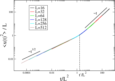
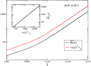
Figure 1: Left panel: $\langle x^{2}(t)\rangle_{0}/L$ vs $t/L^{2}$ is plotted for several values of $L$ in the comb model. Right panel: $\langle x^{2}(t)\rangle_{0}$ and the response function $\overline{\delta x}(t)$ for $L=512$. In the inset the parametric plot $\overline{\delta x}(t)$ vs $\langle x^{2}(t)\rangle_{0}$ is shown.

In the limit of infinite teeth, $L\rightarrow\infty$, $D\rightarrow 0$ and $t^{*}\rightarrow\infty$ and the system shows a pure subdiffusive behaviour [44]

$$\langle x^{2}(t)\rangle_{0}\sim t^{1/2}.$$ (39)

In this case, the probability distribution function behaves as

$$P_{0}(x,t)\sim t^{-1/4}e^{-c\left(\frac{|x|}{t^{1/4}}\right)^{4/3}},$$ (40)

where $c$ is a constant, in agreement with an argument à la Flory [31]. The behaviour (40) also holds in the case of finite $L$, provided that $t<t^{*}$. For larger times a simple Gaussian distribution is observed.

In the comb model with infinite teeth, the FDR in its standard form is fulfilled, namely if we apply a constant perturbation $\varepsilon$ pulling the particles along the 1-d lattice one has numerical evidence that

$$\langle x^{2}(t)\rangle_{0}\simeq C\overline{\delta x}(t)\sim t^{1/2},$$ (41)

where $\overline{\delta x}$ is the average in the presence of the perturbation $\varepsilon$. Moreover, the proportionality between $\langle x^{2}(t)\rangle_{0}$ and $\overline{\delta x}(t)$ is fulfilled also with $L<\infty$, where both the mean square displacement (MSD) and the drift with an applied force exhibit the same crossover from subdiffusive, $\sim t^{1/2}$, to diffusive behavior, $\sim t$ (see Fig. 1, right panel). Therefore what we can say is that the FDR is somehow “blind” to the dynamical crossover experienced by the system. When the perturbation is applied to a state without any current, the proportionality between response and correlation holds despite anomalous transport phenomena.

3.4 Application of the generalized FDR

Our aim here is to show that, differently from what depicted above about the zero current situation, within a state with a non zero drift the emergence of a dynamical crossover is connected to the breaking of the Einstein FDR (4). Indeed, the MSD in the presence of a non zero current, even with $L=\infty$, shows a dynamical crossover

$$\langle x^{2}(t)\rangle_{d} \sim a~{}t^{1/2}+b~{}t,$$ (42)

$$\langle[x(t)-\langle x(t)\rangle_{d}]^{2}\rangle_{d} \sim a^{\prime}~{}t^{1/2}+b^{\prime}~{}t,$$ (43)

where $a$, $b$, $a^{\prime}$ and $b^{\prime}$ are constants, whereas

$$\overline{\delta x}_{d}(t)\sim t^{1/2},$$ (44)

with $\overline{\delta x}_{d}(t)=\langle x(t)\rangle_{d+\varepsilon}-\langle x(t)\rangle_{d}$: hence at large times the Einstein relation breaks down (see Fig. 2). Notice that the proportionality between response and fluctuations cannot be recovered by simply replacing $\langle x^{2}(t)\rangle_{d}$ with $\langle x^{2}(t)\rangle_{d}-\langle x(t)\rangle^{2}_{d}$, as it happens for Gaussian processes (see discussion below). The constants $a^{\prime}$ and $b^{\prime}$ can be computed analitically in the case $L=\infty$ [45].

The first moment $\langle x(t)\rangle_{d+\varepsilon}$ of $P_{d+\varepsilon}(x,t)$ is not proportional to the second cumulant of $P_{d}(x,t)$, namely $\langle x^{2}(t)\rangle_{d}-\langle x(t)\rangle^{2}_{d}$. In order to point out a relation between such quantities, we need a generalized fluctuation-dissipation relation.

According to the definition (38), one has for the backbone

$$W^{d+\varepsilon}[(x,y)\rightarrow(x^{\prime},y^{\prime})] = W^{d}[(x,y)\rightarrow(x^{\prime},y^{\prime})]\left(1+\frac{\varepsilon(x^{\prime}-x)}{W^{0}+d(x^{\prime}-x)}\right)$$

$$\simeq W^{d}e^{\frac{\varepsilon}{W^{0}}(x^{\prime}-x)},$$

where $W^{0}=1/4$, and the last expression holds under the condition $d/W^{0}\ll 1$. The above expression can be rewritten in the form of a local detailed balance, Eq. (24), with $V({\bf x})=x$ and $\beta=1$, yielding, for $(x,y)\neq(x^{\prime},y^{\prime})$,

$$W^{d+\varepsilon}[(x,y)\rightarrow(x^{\prime},y^{\prime})]=W^{d}[(x,y)\rightarrow(x^{\prime},y^{\prime})]e^{\frac{h(\varepsilon)}{2}(x^{\prime}-x)},$$ (47)

where $h(\varepsilon)=2\varepsilon/W^{0}$. Using Eqs. (30) and (31) we obtain

$$\frac{\overline{\delta\mathcal{O}}_{d}}{h(\varepsilon)}=\frac{\langle\mathcal{O}(t)\rangle_{d+\varepsilon}-\langle\mathcal{O}(t)\rangle_{d}}{h(\varepsilon)}=\frac{1}{2}\left[\langle\mathcal{O}(t)x(t)\rangle_{d}-\langle\mathcal{O}(t)x(0)\rangle_{d}-\langle\mathcal{O}(t)A(t,0)\rangle_{d}\right],$$ (48)

where $\mathcal{O}$ is a generic observable, and $A(t,0)=\sum_{t^{\prime}=0}^{t}B(t^{\prime})$, with, in this case,

$$B[(x,y)]=\sum_{(x^{\prime},y^{\prime})}(x^{\prime}-x)W^{d}[(x,y)\rightarrow(x^{\prime},y^{\prime})].$$ (49)

Recalling the definitions (38), from the above equation we have $B[(x,y)]=2d\delta_{y,0}$ and therefore the sum on $B$ has an intuitive meaning: it counts the time spent by the particle on the $x$ axis. The results described in section 3.3 can be then read in the light of the fluctuation-dissipation relation (48):

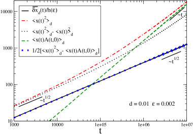
Figure 2: Response function (black line), MSD (red dotted line) and second cumulant (black dotted line) measured in the the comb model with $L=\infty$, field $d=0.01$ and perturbation $\varepsilon=0.002$. The correlation involving the quantity $B$ (green dotted line) yields the right correction to recover the full response function (blue dotted line), in agreement with the FDR (48).

i) Putting $\mathcal{O}(t)=x(t)$, in the case without drift, i.e. $d=0$, one has $B=0$ and, recalling the choice of the initial condition $x(0)=0$,

$$\frac{\overline{\delta x}}{h(\varepsilon)}=\frac{\langle x(t)\rangle_{\varepsilon}-\langle x(t)\rangle_{0}}{h(\varepsilon)}=\frac{1}{2}\langle x^{2}(t)\rangle_{0}.$$ (50)

This explains the observed behaviour (41) even in the anomalous regime and predicts the correct proportionality factor, $\overline{\delta x}(t)=\varepsilon/W^{0}\langle x^{2}(t)\rangle_{0}$.

ii) Putting $\mathcal{O}(t)=x(t)$, in the case with $d\neq 0$, one has

$$\frac{\overline{\delta x}_{d}}{h(\varepsilon)}=\frac{1}{2}\left[\langle x^{2}(t)\rangle_{d}-\langle x(t)A(t,0)\rangle_{d}\right].$$ (51)

This explains the observed behaviours (42) and (44): the leading behavior at large times of $\langle x^{2}(t)\rangle_{d}\sim t$, turns out to be exactly canceled by the term $\langle x(t)A(t,0)\rangle_{d}$, so that the relation between response and unperturbed correlation functions is recovered (see Fig. 2).

iii) As discussed above, it is not enough to substitute $\langle x^{2}(t)\rangle_{d}$ with $\langle x^{2}(t)\rangle_{d}-\langle x(t)\rangle_{d}^{2}$ to recover the proportionality with $\overline{\delta x}_{d}(t)$ when the process is not Gaussian. This can be explained in the following manner. By making use of the second order out of equilibrium FDR derived by Lippiello et al. in [46, 47, 48], which is needed due to the vanishing of the first order term for symmetry, we can explicitly evaluate

$$\langle x^{2}(t)\rangle_{d}=\langle x^{2}(t)\rangle_{0}+h^{2}(d)\frac{1}{2}\left[\frac{1}{4}\langle x^{4}(t)\rangle_{0}+\frac{1}{4}\langle x^{2}(t)A^{(2)}(t,0)\rangle_{0}\right],$$ (52)

where $A^{(2)}(t,0)=\sum_{t^{\prime}=0}^{t}B^{(2)}(t^{\prime})$ with $B^{(2)}=-\sum_{x^{\prime}}(x^{\prime}-x)^{2}W[(x,y)\rightarrow(x^{\prime},y^{\prime})]=-1/2\delta_{y,0}$. Then, recalling Eq. (50), we obtain

$$\langle x^{2}(t)\rangle_{d}-\langle x(t)\rangle^{2}_{d}=$$

$$\langle x^{2}(t)\rangle_{0}+h^{2}(d)\left[\frac{1}{8}\langle x^{4}(t)\rangle_{0}+\frac{1}{8}\langle x^{2}(t)A^{(2)}(t,0)\rangle_{0}-\frac{1}{4}\langle x^{2}(t)\rangle^{2}_{0}\right].$$ (53)

Numerical simulations show that the term in the square brackets grows like $t$ yielding a scaling behaviour with time consistent with Eq. (43). On the other hand, in the case of the simple random walk, one has $B^{(2)}=-1$ and $A^{(2)}(t,0)=-t$ and then

$$\langle x^{2}(t)\rangle_{d}-\langle x(t)\rangle^{2}_{d}=$$

$$\langle x^{2}(t)\rangle_{0}+h^{2}(d)\left[\frac{1}{8}\langle x^{4}(t)\rangle_{0}-\frac{1}{8}t\langle x^{2}(t)\rangle_{0}-\frac{1}{4}\langle x^{2}(t)\rangle^{2}_{0}\right].$$ (54)

Since in the Gaussian case $\langle x^{4}(t)\rangle_{0}=3\langle x^{2}(t)\rangle^{2}_{0}$ and $\langle x^{2}(t)\rangle_{0}=t$, the term in the square brackets vanishes identically and that explains why, in the presence of a drift, the second cumulant grows exactly as the second moment with no drift.

4 Entropy Production

Non equilibrium regimes are always characterized by some sort of current flowing across the systems. In the following sections we will suggest, showing examples, some connections between such non-equilibrium currents and the new degrees of freedom entering the fluctuation dissipation relation, while in the present one we introduce a general symmetry relation of the probability distribution of such currents, the Fluctuation relation.

In general, when one deals with non-equilibrium dynamics, very few results independent from the details of the model are available. Actually in the last decade a group of relations, known with the name of “fluctuation relations” have captured the interest of the scientific community, especially for the vast range of applicability. Initially, a numerical evidence given by Evans and collaborators showed a particular symmetry in the distribution of an observable of a molecular fluid under shear. In a second moment, such a symmetry has been proved as a theorem by Gallavotti and Cohen, under quite general hypothesis. The interested reader can see, among others [49]. For a review of large deviation theory applied to non-equilibrium systems, see [50].

According to the point of view here adopted we will focus on systems in which some randomness is present. Thanks to this assumption, it is possible to skip several technical problems and some forms of fluctuation theorems for stochastic systems can be used. Among others, we are going to use the Lebowitz-Spohn functional, valid for Markovian dynamics. In order to fix ideas, let us consider a one-dimensional process discrete in time (the generalization to the other cases is straightforward) and let us identify a trajectory in a time interval $[0,t]$:

$$\Omega_{t}=\{x(0),x(1),\dots,x(t)\}$$ (55)

Clearly, because of the stochastic nature of the dynamics it is possible to associate to the trajectories a probability $P(\Omega_{t})$; using the Markovian nature of the process one has

$$P(\Omega_{t})=p(x(0))\prod_{n=1}^{t}W(x(n-1)\to x(n))$$ (56)

Analogously, one can consider the time-reversed trajectory, i.e. $\overline{\Omega}_{t}={x(t),x(t-1),\dots,x(0)}$ with its probability $P(\overline{\Omega_{t}})$. For clarity, here we are considering variables which are even in time. This is not the most general case: for example, when one deals also with velocities one must take into account the different parity of the variables. Then the Lebowitz-Spohn functional is defined as

$$\Sigma_{t}=\log{\frac{P(\Omega_{t})}{P(\overline{\Omega}_{t})}}.$$ (57)

Note that this quantity, in general, is not related to a specific thermodynamic observable. However, in what follows, we will call it “entropy production” according to the recent literature. If the dynamics satisfies detailed balance conditions, one has that $P(\Omega_{t})=P(\overline{\Omega}_{t})$ and then $\Sigma_{t}$ is identically equal to zero. On the contrary, when the detailed balance condition is broken its average is strictly positive and does increase in time

$$\langle\Sigma_{t}\rangle\sim t\phantom{mmmmmm}\textrm{for $t$ large}$$ (58)

where the brackets mean an average on the space of trajectories in the stationary ensemble. In this sense, one of the main features of this quantity is that it captures the “non-equilibrium” nature of the system.

Let us discuss with a pedagogical example how the entropy production is related to non-equilibrium currents. Consider a Markov process where the perturbation of an external force $F$ inducing non-equilibrium currents enters in the transition rates according to local detailed balance condition

$$\frac{W_{F}(x\rightarrow x^{\prime})}{W_{F}(x^{\prime}\rightarrow x)}=\frac{W_{0}(x\rightarrow x^{\prime})}{W_{0}(x^{\prime}\rightarrow x)}e^{2\beta Fj(x\rightarrow x^{\prime})},$$ (59)

with $j(x\rightarrow x^{\prime})$ the current associated to the transition $x\rightarrow x^{\prime}$, which obey the symmetry property $j(x\rightarrow x^{\prime})=-j(x^{\prime}\rightarrow x)$. According to the definition of entropy production (57) one finds, for large times,

$$\frac{\Sigma_{t}}{t}=2\beta F\frac{1}{t}\sum_{n=1}^{t}J(x(n-1)\to x(n))=2\beta FJ(t),$$ (60)

where $J(t)$ is the average current over a time window of duration $t$. The fluctuation theorem is a symmetry property of the probability distribution of the variable $y=\Sigma_{t}/t$ which reads:

$$\frac{P(y)}{P(-y)}=e^{y}\Longrightarrow\frac{P(2\beta FJ(t))}{P(-2\beta FJ(t))}=e^{2\beta FJ(t)}.$$ (61)

Namely the fluctuation theorem describes a symmetry in the fluctuations of currents. Also, for large times we can assume a large deviation hypothesis $P(y)\sim e^{-tS(y)}$, with $S(y)$ a Cramer function. For small fluctuations around the mean value of $y$ the Cramer function can be approximated to $S(y)=S(2\beta FJ)\simeq\beta^{2}F^{2}(J-\overline{J})^{2}/\sigma_{J}^{2}$, where $\sigma_{J}$ is the variance. The fluctuation relation reads as $S(y)-S(-y)=y$; in the Gaussian limit ($y$ close to $\overline{y}$) the previous constraint can be easily demonstrated to be equivalent to $\overline{J}/F=\beta\sigma_{J}^{2}$, which is nothing but the standard fluctuation dissipation relation. Therefore the fluctuation relation, which in some simple situation can be directly related to the fluctuation-dissipation relation, is a more general symmetry to which we expect to obey the fluctuating entropy production. For a more general discussion of the link between the Lebowitz-Spohn entropy production and currents, see [51, 52]. The remarkable fact appearing in equation (61) is that it does not contain any free parameter, and so, in this sense, is model-independent.

5 Langevin processes without detailed balance

Sometimes the properties of statistical systems are investigated studying the diffusional properties of probe particles which customarily have larger mass and size compared with the constituents of the environment. This is for instance the case of Brownian motion, in which the erratic motion of flower-dust within water molecules was considered. The central point is that such probe particle is always coupled to a small portion of the whole system, so that small scale fluctuations always do matter. We are going to study the feedback of local fluctuations of the fluid surrounding the probe on the dynamics of the probe itself when the environment is out of equilibrium. The dynamics of a single probe particle in contact with an equilibrium thermal bath is well described by a single stochastic differential equation:

$$M\dot{V}(t)=-\int_{-\infty}^{t}dt^{\prime}~{}\Gamma(t-t^{\prime})V(t^{\prime})+{\cal E}(t^{\prime}),$$ (62)

where ${\cal E}(t)$ is a gaussian white noise with zero mean and variance $\langle{\cal E}(t){\cal E}(t^{\prime})\rangle=\Gamma(|t-t^{\prime}|)$ (second kind FDT). The equilibrium condition is always guaranteed by the proportionality between memory kernel and noise autocorrelation. The simpler way to account for the coupling between our probe particle with non equilibrium fluctuations of the environments is by breaking the second kind FDT.

In the rest of the section, we will discuss the following points:

• how non-equilibrium arises in a multidimensional linear Langevin model;

• how the coupling between the variable of interest and others do matter in the response formula;

• what form is taken by the Fluctuation-Relation in such a system.

5.1 Markovian linear system

The coupling between the probe and the portion of fluid surrounding it, Eq. (62), in certain regimes may be effectively described in terms of two coupled Langevin equations: one variable is the velocity of our tagged particle and the other is a local force field. Such a simplification can be realized in not too dense cases, where the memory kernel $\Gamma$ has a single characteristic finite time: a more detailed discussion can be found in [53, 54] and a specific example, in the context of granualr systems, is given in section 6. The system can be then put in the following form [55]:

$$M\dot{V} = -\Gamma(V-U)+\sqrt{2\Gamma T_{1}}\phi_{1}$$ (63)

$$M^{\prime}\dot{U} = -\Gamma^{\prime}U-\Gamma V+\sqrt{2\Gamma^{\prime}T_{2}}\phi_{2},$$

where $M$ and $M^{\prime}$ are “masses”, $\Gamma$ and $\Gamma^{\prime}$ are sort of viscosities and $T_{1}$ and $T_{2}$ are two different “energy scales”.

Model (63), in a more compact form, reads

$$\frac{d\bf X}{dt}=-A{\bf X}+{\bf\phi},$$ (64)

where ${\bf X}\equiv(X_{1},X_{2})$ e ${\bf\phi}\equiv(\phi_{1},\phi_{2})$ are 2-dimensional vectors and $A$ is a real $2\times 2$ matrix and ${\bf\phi}(t)$ a Gaussian process, with zero mean and covariance matrix:

$$\left<\phi_{i}(t^{\prime})\phi_{j}(t)\right>=2\delta(t-t^{\prime})D_{ij},$$ (65)

and

$$A=\left(\begin{array}[]{cc}\frac{\Gamma}{M}&-\frac{\Gamma}{M}\\ \frac{\Gamma}{M^{\prime}}&\frac{\Gamma^{\prime}}{M^{\prime}}\end{array}\right)\phantom{mmmmm}D=\left(\begin{array}[]{cc}\frac{\Gamma T_{1}}{M^{2}}&0\\ 0&\frac{\Gamma^{\prime}T_{2}}{(M^{\prime})^{2}}\end{array}\right).$$ (66)

The stability conditions on the dynamical matrix which guarantee the existence of a stationary state are $\textrm{Tr}(A)>0$ and $\textrm{det}(A)>0$ which are clearly fulfilled in the present case. The invariant measure of the steady state is represented by a $2$-variate Gaussian distribution:

$$\rho({\bf X})=N\exp{\left(-\frac{1}{2}{\bf X}\sigma^{-1}{\bf X}\right)}$$ (67)

where $N$ is a normalization coefficient and the matrix of covariances $\sigma$ is obtained by solving

$$D=A\sigma+\sigma A^{T},$$ (68)

which yields:

$$\sigma=\left(\begin{array}[]{cc}\frac{T}{M}+\Theta\Delta T&\Theta\Delta T\\ \Theta\Delta T&\frac{T_{1}}{M^{\prime}}+\frac{\Gamma}{\Gamma^{\prime}}\Theta\Delta T\\ \end{array}\right)$$ (69)

where $\Theta=\frac{\Gamma\Gamma^{\prime}}{(\Gamma+\Gamma^{\prime})(M^{\prime}\Gamma+M\Gamma^{\prime})}$ and $\Delta T=T_{1}-T_{2}$. It is now well clear that when $T_{1}=T_{2}$ the two variables are uncorrelated. This is the fingerprint of an equilibrium condition, as we shall see in the following sections.

5.2 Fluctuation-response relation

We can now explicitly study the fluctuation and response properties of the system since the dynamics is linear. First, the correlation matrix $C_{ij}(t,t^{\prime})=\langle X_{i}(t)X_{j}(t^{\prime})\rangle$, in the stationary state is time-translational invariant, i.e. it only depends on the time difference $t-t^{\prime}$. Then, using the equation of motion, it is immediate to verify that $\dot{C}(t)=-AC(t)$, with initial condition given by the covariance matrix, i.e. $C(0)=\sigma$. The corresponding solution (in the matrix form) is: $C(t)=e^{-At}\sigma$ Note that, in general $\sigma$ and $A$ do not commute. Moreover, considering the gaussian shape of the steady state distribution function (67) it is possible to calculate the response function of the system, by a straightforward application of (17):

$${\bf R}(t)\equiv\overline{\frac{\delta X_{i}(t)}{\delta X_{j}(0)}}=\sum_{i,j}\sigma^{-1}_{ij}\langle X_{i}(t)X_{j}(0)\rangle={\bf C}(t)\sigma^{-1}.$$ (70)

In the case of our interest, by considering a perturbation applied to the variable $V$, one obtains:

$$\overline{\frac{\delta V(t)}{\delta V(0)}}=\sigma^{-1}_{11}\langle V(t)V(0)\rangle+\sigma^{-1}_{21}\langle V(t)U(0)\rangle.$$ (71)

As it appears clear from equation (71), the response of the variable $V$ to an external perturbation in general is not proportional to the unperturbed autocorrelation. It is possible to observe the following scenario: in the case $T_{1}=T_{2}\equiv T$, i.e. $\Delta T=0$, $\sigma$ is diagonal with $\sigma_{11}=\frac{T}{M}$ and $\sigma_{22}=\frac{T}{M^{\prime}}$, independently of the values of other parameters, a direct proportionality between $C_{VV}$ and $R_{VV}$ is obtained. This is not the only case for this to happen: also for $\Gamma\ll\Gamma^{\prime}$, or $\Gamma\gg\Gamma^{\prime}$, $\sigma_{12}$ goes to zero and a direct proportionality between response and autocorrelation of velocity is recovered. More in general, when $T_{2}\neq T_{1}$, the coupling term $\sigma_{12}$ differs from zero and a “violation” of the Einstein relation emerges, triggered by the coupling between different degrees of freedom.

The situation is clarified by Fig. 3, where the Einstein Relation is violated and the generalized FDR holds: response $R_{VV}(t)$, when plotted against $C_{VV}(t)$, shows a non-linear (and non-monotonic) graph. Anyway a simple linear plot is restored when the response is plotted against the linear combination of correlations indicated by formula (71). In this case it is evident that the “violation” cannot be interpreted by means of any effective temperature [56]: on the contrary it is a consequence of having “missed” the coupling between variables $V$ and $U$, which gives an additive contribution to the response of $V$.

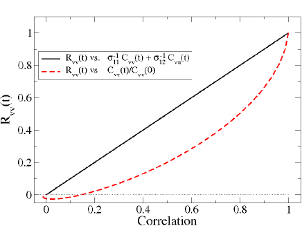
Figure 3: Free particle with viscosity and memory, whose dynamics is given by Eq. (63): here we show the parametric plot of the velocity response to an impulsive perturbation at time $0$, versus two different correlations. The Einstein relation, which is not satisfied, would correspond to a linear shape with slope $1$ for the red dashed line. The black line shows that the Generalized response relation holds.

The above consideration can be easily generalized to the case where several auxiliary fields are present: let us suppose that there are $N-1$ variables at temperature $T_{1}$ (the velocity $V$ and $N-2$ auxiliary variables $U_{i}$) and one at temperature $T_{2}$. In this case it is possible to show that the off-diagonal terms in $\sigma$ are proportional to $(T_{1}-T_{2})$ and a qualitative similar analysis can be performed.

It is useful to stress the role of Markovianity, which is relevant for a correct prediction of the response. In fact the marginal probability distribution of velocity $P_{m}(V)$ can be computed straightforwardly and has always a Gaussian shape. By that, one could be tempted to conclude, inserting $P_{m}(V)$ inside , that proportionality between response and correlation holds also if $T_{2}\neq T_{1}$. This conclusion is wrong, as shown in equation (20) because the process is Markovian only if both the variable $V$ and the ”hidden” variable $U$ are considered.

We conclude by mentioning a sentence of Onsager: how do you know you have taken enough variables, for it to be Markovian? [57]. We have seen in this section how a correct Response-Fluctuation analisys is intimately related to this important caveat.

5.3 Entropy production

Due to the linearity of the model (64), the explicit calculation of the entropy production according to the Lebowitz-Spohn definition is quite straightforward. There is a one to one mapping between the trajectories of the system and the realizations of the noise which allows to write the probability of each trajectory as a path-integral over all the possible realizations of noise:

$$P(\{{\bf X}(s)\}_{0}^{t})=\int\mathcal{D}{\bf\phi}P({\bf\phi})\delta(\dot{{\bf X}}+A{\bf X}-\phi)\,.$$ (72)

Due to the gaussianity of $P(\phi)$ the above integral is easily evaluated yielding the well know Onsager-Machlup expression for the path probabilities:

$$P(\{{\bf X}(s)\}_{0}^{t})\sim e^{-(\dot{{\bf X}}+A{\bf X})D^{-1}(\dot{{\bf X}}+A{\bf X})}.$$ (73)

In our model it is possible to compute the entropy production functional of a single trajectory. Let us consider a general trajectory $\{{\bf X}(s)\}_{0}^{t}$ and its time-reversal $\{\overline{{\bf X}}(s)\}_{0}^{t}$. Lebowitz and Spohn defined a fluctuating entropy production functional $W_{t}$ as follows [52]:

$$\Sigma_{t}^{\prime}=\log\frac{p[{\bf X}(0)]P(\{{\bf X}(s)\}_{0}^{t})}{p[{\bf X}(t)]P(\{\overline{{\bf X}}(s)\}_{0}^{t})}=W_{t}+b_{t}$$ (74)

with

$$b_{t}=\log\{f[{\bf X}(0)]\}-\log\{f[({\bf X})]\},$$ (75)

where $p[{\bf X}(0)]$ is the stationary distribution, i.e. a bivariate gaussian with covariance given by equation (68). Lebowitz and Sphon have shown that the average (over the steady ensemble) of $W_{t}$, if detailed balance is not satisfied, increases linearly with time, while the term $b_{t}$, usually known as “border term”, is usually negligible for large times, unless particular conditions of “singularity” occur [58, 59, 60].

For semplicity of the notation, let us define $\left(\begin{array}[]{c}F_{1}(\textbf{X})\\ F_{2}(\textbf{X})\end{array}\right)\equiv-A\textbf{X}$. In order to write down an explicit expression for the entropy production, it is necessary to establish parity of variables under time-reversal (i.e. positions are even and velocities are odd under time inversion transformation). Let us assume that under time reversal $\overline{X_{i}}=\epsilon_{i}X_{i}$, where $\epsilon_{i}$ can be $+1$ or $-1$, using also $\epsilon{\bf X}\equiv(\epsilon_{1}X_{1},\epsilon_{2}X_{2})$. Then it is possible to define

$$F_{i}^{rev}(\textbf{X}) = \frac{1}{2}[F_{i}(\textbf{X})-\epsilon_{i}F_{i}(\epsilon{\bf X})]=-\epsilon_{i}F_{i}^{rev}(\epsilon{\bf X})$$ (76)

$$F_{i}^{ir}(\textbf{X}) = \frac{1}{2}[F_{i}(\textbf{X})+\epsilon_{i}F_{i}(\epsilon{\bf X})]=\epsilon_{i}F_{i}^{ir}(\epsilon{\bf X}).$$ (77)

Given this notation [61] it is possible to write down a compact form for the entropy production by simply substituting equation (73) into (74) and obtaining:

$$\Sigma_{t}=\sum_{k}D^{-1}_{kk}\int_{0}^{t}dsF^{ir}_{k}\left[\dot{X}_{k}-F^{rev}_{k}\right],$$ (78)

where the sum is over $k$ such that $D_{kk}\neq 0$. Formula (78) is valid also in presence on non-linear terms and with several variables [54].

For the model system in Eq. (63), it appears clear that the variable $V$, being velocity, is odd under the change of time, while variable $U$, which represents the local force field (divided by $\Gamma$), is even. According to the above formula the entropy production reads as:

$$\Sigma_{t}\simeq\Gamma\left(\frac{1}{T_{2}}-\frac{1}{T_{1}}\right)\int_{0}^{t}V(t^{\prime})U(t^{\prime})dt^{\prime}.$$ (79)

Note that, from (79), one recovers the equilibrium case, i.e. $T_{1}=T_{2}$, for which there is no entropy production. Remarkably, the equality of the two temperatures is the same equilibrium condition given by the FDT analysis.

6 Granular intruder

Models of granular fluids [62] are an interesting framework where the issues discussed in the previous sections can be addressed. Due to dissipative interactions among the microscopic constituents, energy is not conserved and external sources are necessary in order to maintain a non-trivial stationary state: time reversal invariance is broken and consequently, properties such as the Equilibrium Fluctuation-Dissipation relation (EFDR) do not hold. In recent years, a rather complete theory for fluctuations in granular systems has been developed for the dilute limit, in good agreement with numerical simulations [63, 64]. However, a general understanding of dense cases is still lacking. A common approach is the so-called Enskog correction [63, 65], which renormalizes the collision frequency to take into account the breakdown of Molecular Chaos due to high density. In cooling regimes, the Enskog theory may describe strong non-equilibrium effects, due to the explicit cooling time-dependence [66]. However it cannot describe dynamical effects in stationary regimes, such as violations of the Einstein relation [67, 68]. Indeed, as discussed before, violations of Einstein relation comes from having neglected coupled degrees of freedom which are expected to be independent at equilibrium. The Enskog approximation is not sufficient to describe the effect of such a coupling, because it does not break factorization of velocities:

$$\rho(x_{1},...x_{N},v_{1},...v_{N})=\rho_{x}(x_{1},...,x_{N})\prod_{i=1}^{N}p_{1}(v_{i})$$ (80)

with $p_{1}(v)$ the single-particle velocity distribution. Such an approximation, which predicts the validity of Einstein relation, is revealed to be wrong already at moderate densities in granular fluids, as discussed in the following.

6.1 Model

A good benchmark for new non-equilibrium theories is provided by the dynamics of a massive tracer interacting with a gas of smaller granular particles, both coupled to an external bath. In particular, taking as a reference point the dilute limit, where the system has a closed analytical description [69], it is shown that more dense configurations are well described by a Generalized Langevin Equation (GLE) with an exponential memory kernel of the form given in Eq. (62), at least as a first approximation capable of describing violations of EFDR and other non-equilibrium properties [55]. Here, the main features are:

• the decay of correlation and response functions is not a simple exponential and shows backscattering [70, 71];

• the EFDR [72, 73] of the first and second kind do not hold.

In the model described here detailed balance is not satisfied in general, non-equilibrium effects can be taken into account and the correct behavior of correlation and response functions is predicted. Furthermore, the model has a remarkable property: it can be mapped onto the two-variable Markovian system discussed in the previous section, i.e. two coupled Langevin equations, as in Eqs. (63). The dilute limit is then naturally recovered by putting to zero the coupling constant between the original variable and the auxiliary one. The auxiliary variable can be identified in the local velocity field spontaneously appearing in the surrounding fluid. This allows us to measure the fluctuating entropy production (see Eq.(57) [74], and fairly verify the Fluctuation Relation (61)  [75, 52, 73], a remarkable result, if considered the interest of the community [76] and compared with unsuccessful past attempts [77, 78].

The model considered here [55] is the following: an “intruder” disc of mass $m_{0}=M$ and radius $R$, moving in a gas of $N$ granular discs with mass $m_{i}=m$ ($i>0$) and radius $r$, in a two dimensional box of area $A=L^{2}$. We denote by $n=N/A$ the number density of the gas and by $\phi$ the occupied volume fraction, i.e. $\phi=\pi(Nr^{2}+R^{2})/A$ and we denote by $\bm{V}$ (or $\bm{v}_{0}$) and $\bm{v}$ (or $\bm{v}_{i}$ with $i>0$) the velocity vector of the tracer and of the gas particles, respectively. Interactions among the particles are hard-core binary instantaneous inelastic collisions, such that particle $i$, after a collision with particle $j$, comes out with a velocity

$$\bm{v}_{i}^{\prime}=\bm{v}_{i}-(1+\alpha)\frac{m_{j}}{m_{i}+m_{j}}[(\bm{v}_{i}-\bm{v}_{j})\cdot\hat{\bm{n}}]\hat{\bm{n}}$$ (81)

where $\hat{\bm{n}}$ is the unit vector joining the particles’ centers of mass and $\alpha\in[0,1]$ is the restitution coefficient ($\alpha=1$ is the elastic case). The mean free path of the intruder is proportional to $l_{0}=1/((r+R)n)$ and we denote by $\tau_{c}$ its mean collision time. Two kinetic temperatures can be introduced for the two species: the gas granular temperature $T_{g}=m\langle\bm{v}^{2}\rangle/2$ and the tracer temperature $T_{tr}=M\langle\bm{V}^{2}\rangle/2$.

In order to maintain a granular medium in a fluidized state, an external energy source is coupled to each particle in the form of a thermal bath [79, 80, 81] (hereafter, exploiting isotropy, we consider only one component of the velocities):

$$m_{i}\dot{v}_{i}(t)=-\gamma_{b}v_{i}(t)+f_{i}(t)+\xi_{b}(t).$$ (82)

Here $f_{i}(t)$ is the force taking into account the collisions of particle $i$ with other particles, and $\xi_{b}(t)$ is a white noise (different for all particles), with $\langle\xi_{b}(t)\rangle=0$ and $\langle\xi_{b}(t)\xi_{b}(t^{\prime})\rangle=2T_{b}\gamma_{b}\delta(t-t^{\prime})$. The effect of the external energy source balances the energy lost in the collisions and a stationary state is attained with $m_{i}\langle v_{i}^{2}\rangle\leq T_{b}$ .

At low packing fractions, $\phi<0.1$, and in the large mass limit, $m/M\ll 1$, using the Enskog approximation it has been shown [69] that the dynamics of the intruder is described by a linear Langevin equation:

$$M\dot{V}=-\Gamma_{E}V+{\cal E}_{E},$$ (83)

where ${\cal E}_{E}$ is a white noise such that

$$\langle{\cal E}_{i}(t){\cal E}_{j}(t^{\prime})\rangle=2\left[\gamma_{b}T_{b}+\gamma_{g}^{E}\left(\frac{1+\alpha}{2}T_{g}\right)\right]\delta_{ij}\delta(t-t^{\prime})$$ (84)

and

$$\Gamma_{E}=\gamma_{b}+\gamma_{g}^{E},\quad\textrm{with}\quad\gamma_{g}^{E}=\frac{g_{2}(r+R)}{l_{0}}\sqrt{2\pi mT_{g}}(1+\alpha)$$ (85)

where $g_{2}(r+R)$ is the pair correlation function for a gas particle and the intruder at contact. In this limit the velocity autocorrelation function shows a simple exponential decay, with characteristic time $M/\Gamma_{E}$. Time-reversal and the EFDR, which are very weakly modified for uniform dilute granular gases [82, 67, 83], become perfectly satisfied for a massive intruder. The temperature of the tracer is computed as $T_{tr}^{E}=(\gamma_{b}T_{b}+\gamma_{g}^{E}\frac{1+\alpha}{2}T_{g})/\Gamma_{E}$. For a general study of a Langevin equation with “two temperatures” but a single time scale (which is always at equilibrium), see also [84].

6.2 Dense case: double Langevin with two temperatures

As the packing fraction is increased, the Enskog approximation is less and less effective in predicting memory effects and the dynamical properties. In particular, velocity autocorrelation $C(t)=\langle V(t)V(0)\rangle/\langle V^{2}\rangle$ and linear response function $R(t)=\overline{\delta V(t)}/\delta V(0)$ (i.e. the mean response at time $t$ to an impulsive perturbation applied at time 0) show an exponential decay modulated in amplitude by oscillating functions [71]. Moreover violations of the EFDR $C(t)=R(t)$ (Einstein relation) are observed for $\alpha<1$ [68, 41].

Molecular dynamics simulations [55] of the system have been performed, giving access to $C(t)$ and $R(t)$, for several different values of the parameters $\alpha$ and $\phi$, see Fig. 4.

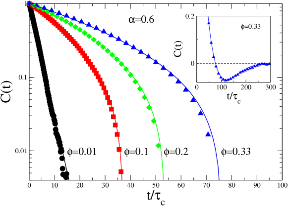
Figure 4: (Color online). Semi-log plot of $C(t)$ (symbols) for different values of $\phi=0.01,0.1,0.2,0.33$ at $\alpha=0.6$. Times are rescaled by the mean collision time $\tau_{c}$. The other parameters are fixed: $N=2500$, $m=1$, $M=25$, $r=0.005$, $R=0.025$, $T_{b}=1$, $\gamma_{b}=200$. Times are rescaled by the mean collision times $\tau_{c}$, as measured in the different cases. Numerical data are averaged over $\sim 10^{5}$ realizations. Continuous lines are the best fits obtained with Eq. (89). Inset: $C(t)$ and the best fit in linear scale for $\phi=0.33$ and $\alpha=0.6$.

Notice that the Enskog approximation [63, 69] cannot predict the observed functional forms, because it only modifies by a constant factor the collision frequency. In order to describe the full phenomenology, a model with more than one characteristic time is needed. The proposed model is a Langevin equation with a single exponential memory kernel [85, 86, 55], as in Eq. (62)

$$M\dot{V}(t)=-\int_{-\infty}^{t}dt^{\prime}~{}\Gamma(t-t^{\prime})V(t^{\prime})+{\cal E}^{\prime}(t),$$ (86)

in this case,

$$\Gamma(t)=2\gamma_{0}\delta(t)+\gamma_{1}/\tau_{1}e^{-t/\tau_{1}}$$ (87)

and ${\cal E}^{\prime}(t)={\cal E}_{0}(t)+{\cal E}_{1}(t)$, with

$$\langle{\cal E}_{0}(t){\cal E}_{0}(t^{\prime})\rangle=2T_{0}\gamma_{0}\delta(t-t^{\prime}),\\ \langle{\cal E}_{1}(t){\cal E}_{1}(t^{\prime})\rangle=T_{1}\gamma_{1}/\tau_{1}e^{-(t-t^{\prime})/\tau_{1}}$$ (88)

and $\langle{\cal E}_{1}(t){\cal E}_{0}(t^{\prime})\rangle=0$. In the limit $\alpha\to 1$, the parameter $T_{1}$ is meant to tend to $T_{0}$ in order to fulfill the EFDR of the $2$nd kind $\langle{\cal E}^{\prime}(t){\cal E}^{\prime}(t^{\prime})\rangle=T_{0}\Gamma(t-t^{\prime})$. Within this model the dilute case is recovered if $\gamma_{1}\to 0$. In this limit, the parameters $\gamma_{0}$ and $T_{0}$ coincide with $\Gamma_{E}$ and $T_{tr}^{E}$ of the Enskog theory [69]. The exponential form of the memory kernel can be justified within the mode-coupling approximation scheme, see [55] for details.

The model (86) predicts $C=f_{C}(t)$ and $R=f_{R}(t)$ with

$$f_{C(R)}=e^{-gt}[\cos(\omega t)+a_{C(R)}\sin(\omega t)].$$ (89)

The variables $g$, $\omega$, $a_{C}$ and $a_{R}$ are known algebraic functions of $\gamma_{0}$, $T_{0}$, $\gamma_{1}$, $\tau_{1}$ and $T_{1}$. In particular, the ratio $a_{C}/a_{R}=[T_{0}-\Omega(T_{1}-T_{0})]/[T_{0}+\Omega(T_{1}-T_{0})]$, with $\Omega=\gamma_{1}/[(\gamma_{0}+\gamma_{1})(\gamma_{0}/M\tau_{1}-1)]$. Hence, in the elastic ($T_{1}\to T_{0}$) as well as in the dilute limit ($\gamma_{1}\to 0$), one gets $a_{C}=a_{R}$ and recovers the EFDR $C(t)=R(t)$. In Fig. 4 the continuous lines show the result of the best fits obtained using Eq. (89) for the correlation function, at restitution coefficient $\alpha=0.6$ and for different values of the packing fraction $\phi$. The functional form fits very well the numerical data. A fit of measured $C$ and $R$ against Eqs. (89), together with a measure of $\langle V^{2}\rangle$, yields five independent equations to determine the five parameters entering the model. We used the external parameters mentioned before, changing $\alpha$ or the box area $A$ (to change $\phi$) or the intruder’s radius $R$, in order to change $\phi$ keeping or not keeping constant $\gamma_{g}\sim 1/l_{0}\to 0$ (indeed different dilute limits can be obtained, where collisions matter or not). Fits from numerical simulations suggest the following identification for the parameters: $\gamma_{0}\sim\Gamma_{E}$, $T_{0}\sim T_{tr}$ and $T_{1}\sim T_{b}$. The coupling time $\tau_{1}$ increases with the packing fraction and, weakly, with the inelasticity. In the most dense cases it appears that $\gamma_{1}\sim\gamma_{g}^{E}\propto\phi$: such an observation however does not hold in the dilute limit at constant collision rate, where $\gamma_{1}\to 0\ll\gamma_{g}^{E}$. It is also interesting to notice that at high density $T_{tr}\sim T_{g}\sim T_{g}^{E}$, which is probably due to the stronger correlations among particles. Finally we notice that, at large $\phi$, $T_{tr}>T_{tr}^{E}$, which is coherent with the idea that correlated collisions dissipate less energy.

Looking for an insight of the relevant physical mechanisms underlying such a phenomenology and in order to make clear the meaning of the parameters, it is useful to map Eq. (86) onto a Markovian equivalent model by introducing an auxiliary field (see [53, 55] for details on how the mapping is achieved):

$$M\dot{V} = -\Gamma_{E}(V-U)+\sqrt{2\Gamma_{E}T_{g}}{\cal E}_{V}$$

$$M^{\prime}\dot{U} = -\Gamma^{\prime}U-\Gamma_{E}V+\sqrt{2\Gamma^{\prime}T_{b}}{\cal E}_{U},$$ (90)

where ${\cal E}_{V}$ and ${\cal E}_{U}$ are indipendent white noises of unitary variance and we have exploited the numerical observations discussed above (i.e. $T_{0}\sim T_{g}$, $T_{1}\sim T_{b}$ and $\gamma_{0}\sim\Gamma_{E}$), while $\Gamma^{\prime}=\frac{\gamma_{0}^{2}}{\gamma_{1}}$ and $M^{\prime}=\frac{\gamma_{0}^{2}\tau_{1}}{\gamma_{1}}$. In the chosen form (90), the dynamics of the tracer is remarkably simple: indeed $V$ follows a memoryless Langevin equation in a Lagrangian frame with respect to a local field $U$, which is the local average velocity field of the gas particles colliding with the tracer. Extrapolating such an identification to higher densities, we are able to understand the value for most of the parameters of the model: the self drag coefficient of the intruder in principle is not affected by the change of reference to the Lagrangian frame, so that $\gamma_{0}\sim\Gamma_{E}$; for the same reason $T_{0}\sim T_{tr}$ is roughly the temperature of the tracer; $\tau_{1}$ is the main relaxation time of the average velocity field $U$ around the Brownian particle; $\gamma_{1}$ is the intensity of coupling felt by the surrounding particles after collisions with the intruder; finally $T_{1}$ is the “temperature” of the local field $U$, easily identified with the bath temperature $T_{1}\sim T_{b}$: indeed, thanks to momentum conservation, inelasticity does not affect the average velocity of a group of particles which almost only collide with themselves.

6.3 Generalized FDR and entropy production

The model discussed above, Eq. (90), is able to reproduce the violations of EFDR, as show in Fig. 5, which depicts correlation and response functions in a dense case (elastic and inelastic). In the inelastic case, deviations from EFDR $R(t)=C(t)$ are observed. In the inset of Fig. 5 the ratio $R(t)/C(t)$ is also reported. As shown in Section 2, a relation between the response and correlations measured in the unperturbed system still exists, but - in the non-equilibrium case - must take into account the contribution of the cross correlation $\langle V(t)U(0)\rangle$, i.e.:

$$R(t)=aC(t)+b\langle V(t)U(0)\rangle$$ (91)

with $a=[1-\gamma_{1}/M(T_{0}-T_{1})\Omega_{a}]$ and $b=(T_{0}-T_{1})\Omega_{b}$, where $\Omega_{a}$ and $\Omega_{b}$ are known functions of the parameters. At equilibrium, where $T_{0}=T_{1}$, the EFDR is recovered.

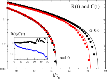
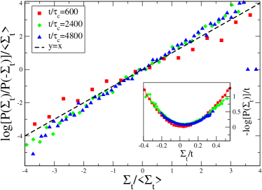
Figure 5: (Color online). Left: correlation function $C(t)$ (black circles) and response function $R(t)$ (red squares) for $\alpha=1$ and $\alpha=0.6$, at $\phi=0.33$. Continuous lines show the best fits curves obtained with Eqs. (89). Inset: the ratio $R(t)/C(t)$ is reported in the same cases. Right: Check of the fluctuation relation (93) in the system with $\alpha=0.6$ and $\phi=0.33$. Inset: collapse of the rescaled probability distributions of $\Sigma_{t}$ at large times onto the large deviation function.

An important independent assessment of the effectiveness of model in Eq. (90) comes from the study of the fluctuating entropy production [74] which quantifies the deviation from detailed balance in a trajectory. Given the trajectory in the time interval $[0,t]$, $\{V(s)\}_{0}^{t}$, and its time-reversed $\{{\cal I}V(s)\}_{0}^{t}\equiv\{-V(t-s)\}_{0}^{t}$, as discussed in section 5.3, shown that the entropy production for the model (90) takes the form [54]

$$\Sigma_{t}=\log\frac{P(\{V(s)\}_{0}^{t})}{P(\{{\cal I}V(s)\}_{0}^{t})}\approx\gamma_{0}\left(\frac{1}{T_{0}}-\frac{1}{T_{1}}\right)\int_{0}^{t}ds~{}V(s)U(s).$$ (92)

This functional vanishes exactly in the elastic case, $\alpha=1$, where equipartition holds, $T_{1}=T_{0}$, and is zero on average in the dilute limit, where $\langle VU\rangle=0$.

Formula (92) reveals that the leading source of entropy production is the energy transferred by the “force” $\gamma_{0}U$ on the tracer, weighed by the difference between the inverse temperatures of the two “thermostats”. Therefore, to measure entropy production, we need to measure the fluctuations of $U$: from the above discussion we have for $U$ the interpretation of a spontaneous local velocity field interacting with the tracer. Therefore it can be measured doing a local average of particles’ velocity in a circle of radius $l$ centered on the tracer. Details on how to choose in a reliable way the proper $l$ are given in [55], for instance following such procedure, in the case $\phi=0.33$ and $\alpha=0.6$, we estimate for the correlation length $l\sim 9r\sim 6l_{0}$. Then, measuring the entropy production from Eq. (92) along many trajectories of length $t$, we can compute the probability $P(\Sigma_{t}=x)$ and compare it to $P(\Sigma_{t}=-x)$, in order to verify the Fluctuation Relation

$$\log\frac{P(\Sigma_{t}=x)}{P(\Sigma_{t}=-x)}=x.$$ (93)

In the right frame of Fig. 5 we report our numerical results. The main frame confirms that at large times the Fluctuation Relation (93) is well verified within the statistical errors. The inset shows the collapse, for large times, of $\log P(\Sigma_{t})/t$ onto the Cramer function $S(y=\frac{\Sigma_{t}}{t})$, introduced in Section 4. Notice also that formula (92) does not contain further parameters but the ones already determined by correlation and response measure, i.e. the slope of the graph is not adjusted by further fits. Indeed a wrong evaluation of the weighing factor $(1/T_{0}-1/T_{1})\approx(1/T_{tr}-1/T_{b})$ or of the “energy injection rate” $\gamma_{0}U(t)V(t)$ in Eq. (92) could produce a completely different slope in Fig. 5 (right frame).

To conclude this section, we stress that velocity correlations $\langle V(t)U(t^{\prime})\rangle$ between the intruder and the surrounding velocity field are responsible for both the violations of the EFDR and the appearance of a non-zero entropy production, provided that the two fields are at different temperatures. We also mention that larger violations of EFDR can be observed using an intruder with a mass equal or similar to that of other particles [68], with the important difference that in such a case a simple “Langevin-like” model for the intruder’s dynamics is not available.

7 Conclusions and perspectives

We have reviewed a series of recent results on fluctuation-dissipation relations for out-of-equilibrium systems. The leitmotiv of our discussion is the importance of correlations for non-equilibrium response, much more relevant than in equilibrium systems: indeed the Generalized Fluctuation-Dissipation relation discussed in Section 3, 5, 6 deviates from its equilibrium counterpart for the appearance of additional contributions coming from correlated degrees of freedom. This is the case, for instance, of the linear response in the diffusion model on a comb-lattice, where - in the presence of a net drift - the linear response takes a non-negligible additive contribution, see Eq. (51). The same occurs in the general two-variable Langevin model: additional contribution to the equilibrium linear response appears when the main field $V$ is coupled to the second field $U$, which only appears out-of-equilibrium, see Eq. (71). The granular intruder is a realistic many-body instance of such a coupling scenario, where we have seen the strong influence of correlated degrees of freedom to the linear response, see Eq. (90).

Remarkably, in some cases, one may explicitly verify that the coupled field which contributes to the linear response in non-equilibrium setups is also involved in the violation of detailed balance: such a violation is measured by the fluctuating entropy production. The connection between non-equilibrium couplings and entropy production has been discussed for general coupled linear Langevin models, see Eq. (79) and then verified for the entropy production of the granular intruder, Eq. (92).

In conclusion many results point in the same direction, suggesting a general framework for linear-response in systems with non-zero entropy production. Even in out-of-equilibrium configurations, a clear connection between response and correlation in the unperturbed systems exists. A further step is looking for more accessible observables which could make easier the prediction of linear response: indeed, both proposed formula, Eq. (13) and Eq. (30), require the measurement of variables which, in general, depend on full phase-space (microscopic) observables and can be strictly model-dependent. Such a difficulty also explains why, in a particular class of slowly relaxing systems with several well separated time-scales, such as spin or structural glasses in the aging dynamics, i.e. after a sudden quench below some dynamical transition temperature, approaches involving “effective temperatures” have been used in a more satisfactory way [87]. More recent interpretations of the additional non-equilibrium contributions has been proposed in [25], but its predictive power is not yet fully investigated and represents an interesting line of ongoing research.

Acknowledgments

We thank A. Baldassarri, F. Corberi, M. Falcioni, E. Lippiello, U. Marini Bettolo Marconi, L. Rondoni and M. Zannetti for a long collaboration on the issues here discussed.

References

- [1] A Einstein. On the movement of small particles suspended in a stationary liquid demanded by the molecular-kinetic theory of heat. Ann. d. Phys., 17:549, 1905.
- [2] L Onsager. Reciprocal relations in irreversible processes. I. Phys. Rev., 37:405–426, 1931.
- [3] L Onsager. Reciprocal relations in irreversible processes. II. Phys. Rev., 38:2265–2279, 1931.
- [4] R Kubo. The fluctuation-dissipation theorem. Rep. Prog. Phys., 29:255, 1966.
- [5] D. J. Evans, E. G. D. Cohen, and G. P. Morriss. Probability of second law violations in shearing steady flows. Phys. Rev. Lett., 71:2401, 1993.
- [6] D J Evans and D J Searles. Steady states, invariant measures, response theory. Phys. Rev. E, 52:5839, 1995.
- [7] G Gallavotti and E G D Cohen. Dynamical ensembles in stationary states. J. Stat. Phys., 80:931, 1995.
- [8] G E Crooks. Path ensemble averages in systems driven far from equilibrium. Phys. Rev. E, 61:2361, 2000.
- [9] C Jarzynski. Nonequilibrium equality for free energy differences. Phys. Rev. Lett., 78:2690, 1997.
- [10] L Boltzmann. Lectures on Gas Theory. Dover, 1995 (1896 first german edition).
- [11] J W Gibbs. Elementary Principles in Statistical Mechanic. Yale University Press, 1902.
- [12] A Einstein. Zur allgemeinen molekularen theorie der wärme. Ann. der Phys., 14:354, 1904.
- [13] J Perrin. Les atomes. Alcan, Paris, 1913.
- [14] P Langevin. Sur la theorie du mouvement brownien. C. R. Acad. Sci. (Paris), 146:530, 1908. translated in Am. J. Phys. 65, 1079 (1997).
- [15] R.H. Rose and P.L. Sulem. Fully developed turbulence and statistical mechanics. J. Phys. (Paris), 39:441, 1978.
- [16] U Deker and F Haake. Fluctuation-dissipation theorems for classical processes. Phys. Rev. A, 11:2043, 1975.
- [17] M Falcioni, S Isola, and A Vulpiani. Correlation functions and relaxation properties in chaotic dynamics and statistical mechanics. Physics Letters A, 144:341, 1990.
- [18] G. Boffetta, G. Lacorata, S. Musacchio, and A. Vulpiani. Relaxation of finite perturbations: Beyond the fluctuation-response relation. Chaos, 13:806, 2003.
- [19] N.G. van Kampen. The case against linear response theory. Phys. Norv., 5:279, 1971.
- [20] R Kubo. Brownian motion and nonequilibrium statistical mechanics. Science, 32:2022, 1986.
- [21] B. Cessac and J.-A. Sepulchre. Linear response, susceptibility and resonance in chaotic toy models. Physica D, 225:13, 2007.
- [22] R. H. Kraichnan. Classical fluctuation-relaxation theorem. Phys. Rev., 113:118, 1959.
- [23] R. H. Kraichnan. Deviations from fluctuation-relaxation relations. Physica A, 279:30, 2000.
- [24] E Lippiello, F Corberi, and M Zannetti. Off-equilibrium generalization of the fluctuation dissipation theorem for Ising spins and measurement of the linear response function. Phys. Rev. E, 71:036104, 2005.
- [25] M Baiesi, C Maes, and B Wynants. Fluctuations and response of nonequilibrium states. Phys. Rev. Lett., 103:010602, 2009.
- [26] F Corberi, E Lippiello, A Sarracino, and M Zannetti. Fluctuation-dissipation relations and field-free algorithms for the computation of response functions. Phys. Rev. E, 81:011124, 2010.
- [27] J R Gomez-Solano, A Petrosyan, S Ciliberto, R Chetrite, and K Gawedzki. Experimental verification of a modified fluctuation-dissipation relation for a micron-sized particle in a non-equilibrium steady state. Phys. Rev. Lett., 103:040601, 2009.
- [28] J R Gomez-Solano, A Petrosyan, S Ciliberto, and C Maes. Fluctuations and response in a non-equilibrium micron-sized system. J. Stat. Mech., page P01008, 2011.
- [29] J L Lebowitz and P G Bergmann. Irreversible gibbsian ensembles. Annals of Physics, 1:1, 1957.
- [30] L F Cugliandolo, J Kurchan, and G Parisi. Off equilibrium dynamics and aging in unfrustrated systems. J. Phys. I, 4:1641, 1994.
- [31] J P Bouchaud and A Georges. Anomalous diffusion in disordered media: Statistical mechanisms, models and physical applications. Phys. Rep., 195:127, 1990.
- [32] Q Gu, E A Schiff, S Grebner, F Wang, and R Schwarz. Non-gaussian transport measurements and the Einstein relation in amorphous silicon. Phys. Rev. Lett., 76:3196, 1996.
- [33] P Castiglione, A Mazzino, P Muratore-Ginanneschi, and A Vulpiani. On strong anomalous diffusion. Physica D, 134:75, 1999.
- [34] R Metzler and J Klafter. The random walk’s guide to anomalous diffusion: a fractional dynamics approach. Phys. Rep., 339:1, 2000.
- [35] R Burioni and D Cassi. Random walks on graphs: ideas, techniques and results. J. Phys. A:Math. Gen., 38:R45, 2005.
- [36] O Bénichou and G Oshanin. Ultraslow vacancy-mediated tracer diffusion in two dimensions: The einstein relation verified. Phys. Rev. E, 66:031101, 2002.
- [37] R Metzler, E Barkai, and J Klafter. Anomalous diffusion and relaxation close to thermal equilibrium: A fractional Fokker-Planck equation approach. Phys. Rev. Lett, 82:3563, 1999.
- [38] E Barkai and V N Fleurov. Generalized Einstein relation: A stochastic modeling approach. Phys. Rev. E, 58:1296, 1998.
- [39] A V Chechkin and R Klages. Fluctuation relations for anomalous dynamics. J. Stat. Mech., page L03002, 2009.
- [40] L Lizana, T Ambjörnsson, A Taloni, E Barkai, and M A Lomholt. Foundation of fractional Langevin equation: Harmonization of a many-body problem. Phys. Rev. E, 81:51118, 2010.
- [41] D Villamaina, A Puglisi, and A Vulpiani. The fluctuation-dissipation relation in sub-diffusive systems: the case of granular single-file diffusion. J. Stat. Mech., page L10001, 2008.
- [42] K Hahn, J Kärger, and V Kukla. Single-file diffusion observation. Phys. Rev. Lett., 76:2762, 1996.
- [43] S Redner. A Guide to First-Passages Processes. Cambridge University Press, 2001.
- [44] S Havlin and D Ben Avraham. Diffusion in disordered media. Adv. Phys., 36:695, 1987.
- [45] E. Barkai. Private communication.
- [46] E Lippiello, F Corberi, A Sarracino, and M Zannetti. Nonlinear susceptibilities and the measurement of a cooperative length. Phys. Rev. B, 77:212201, 2008.
- [47] E Lippiello, F Corberi, A Sarracino, and M Zannetti. Nonlinear response and fluctuation-dissipation relations. Phys. Rev. E, 78:041120, 2008.
- [48] F Corberi, E Lippiello, A Sarracino, and M Zannetti. Fluctuations of two-time quantities and non-linear response functions. J. Stat. Mech., page P04003, 2010.
- [49] D J Evans and D J Searles. The fluctuation theorem. Adv. Phys., 52:1529, 2002.
- [50] H Touchette and R Harris. Large deviation approach to nonequilibrium systems. In the present volume.
- [51] D Andrieux and P Gaspard. Fluctuation theorem for currents and schnakenberg network theory. J. Stat. Phys., 127:107, 2007.
- [52] J L Lebowitz and H Spohn. A Gallavotti-Cohen-type symmetry in the large deviation functional for stochastic dynamics. J. Stat. Phys., 95:333, 1999.
- [53] D Villamaina, A Baldassarri, A Puglisi, and A Vulpiani. Fluctuation dissipation relation: how does one compare correlation functions and responses? J. Stat. Mech., page P07024, 2009.
- [54] A Puglisi and D Villamaina. Irreversible effects of memory. Europhys. Lett., 88:30004, 2009.
- [55] A Sarracino, D Villamaina, G Gradenigo, and A Puglisi. Irreversible dynamics of a massive intruder in dense granular fluids. Europhys. Lett., 92:34001, 2010.
- [56] L F Cugliandolo, J Kurchan, and L Peliti. Energy flow, partial equilibration, and effective temperatures in systems with slow dynamics. Phys. Rev. E, 55:3898, 1997.
- [57] L Onsager and S Machlup. Fluctuations and irreversible processes. Phys. Rev., 91:1505, 1953.
- [58] R van Zon and E G D Cohen. Extension of the fluctuation theorem. Phys. Rev. Lett., 91:110601, 2003.
- [59] A Puglisi, L Rondoni, and A Vulpiani. Relevance of initial and final conditions for the fluctuation relation in markov processes. J. Stat. Mech., page P08010, 2006.
- [60] F Bonetto, G Gallavotti, A Giuliani, and F Zamponi. Chaotic hypothesis, fluctuation theorem, singularities. J. Stat. Phys., 123:39, 2006.
- [61] H Risken. The Fokker-Planck equation: Methods of solution and applications. Springer- Verlag, Berlin, 1989.
- [62] H. M. Jaeger, S. R. Nagel, and R. P. Behringer. Granular solids, liquids, and gases. Rev. Mod. Phys., 68:1259, 1996.
- [63] N K Brilliantov and T Poschel. Kinetic Theory of Granular Gases. Oxford University Press, 2004.
- [64] J J Brey, P Maynar, and M I Garcia de Soria. Fluctuating hydrodynamics for dilute granular gases. Phys. Rev. E, 79:051305, 2009.
- [65] J W Dufty and A Santos. Dynamics of a hard sphere granular impurity. Phys. Rev. Lett., 97:058001, 2006.
- [66] A Santos and J W Dufty. Critical behavior of a heavy particle in a granular fluid. Phys. Rev. Lett., 86:4823, 2001.
- [67] V Garzó. On the Einstein relation in a heated granular gas. Physica A, 343:105, 2004.
- [68] A Puglisi, A Baldassarri, and A Vulpiani. Violations of the Einstein relation in granular fluids: the role of correlations. J. Stat. Mech., page P08016, 2007.
- [69] A Sarracino, D Villamaina, G Costantini, and A Puglisi. Granular brownian motion. J. Stat. Mech., page P04013, 2010.
- [70] A V Orpe and A Kudrolli. Phys. Rev. Lett., 98:238001, 2007.
- [71] A Fiege, T Aspelmeier, and A Zippelius. Long-time tails and cage effect in driven granular fluids. Phys. Rev. Lett., 102:098001, 2009.
- [72] R Kubo, M Toda, and N Hashitsume. Statistical physics II: Nonequilibrium stastical mechanics. Springer, 1991.
- [73] U Marini Bettolo Marconi, A Puglisi, L Rondoni, and A Vulpiani. Fluctuation-dissipation: Response theory in statistical physics. Phys. Rep., 461:111, 2008.
- [74] U Seifert. Entropy production along a stochastic trajectory and an integral fluctuation theorem. Phys. Rev. Lett., 95:040602, 2005.
- [75] J Kurchan. Fluctuation theorem for stochastic dynamics. J. Phys. A, 31:3719, 1998.
- [76] F Bonetto, G Gallavotti, A Giuliani, and F Zamponi. Fluctuations relation and external thermostats: an application to granular materials. J. Stat. Mech., page P05009, 2006.
- [77] K Feitosa and N Menon. Fluidized granular medium as an instance of the fluctuation theorem. Phys. Rev. Lett., 92:164301, 2004.
- [78] A Puglisi, P Visco, A Barrat, E Trizac, and F van Wijland. Fluctuations of internal energy flow in a vibrated granular gas. Phys. Rev. Lett., 95:110202, 2005.
- [79] D R M Williams and F C MacKintosh. Driven granular media in one dimension: Correlations and equation of state. Phys. Rev. E, 54:R9, 1996.
- [80] T P C van Noije, M H Ernst, E Trizac, and I Pagonabarraga. Randomly driven granular fluids: Large-scale structure. Phys. Rev. E, 59:4326, 1999.
- [81] A Puglisi, V Loreto, U M B Marconi, A Petri, and A Vulpiani. Clustering and non-gaussian behavior in granular matter. Phys. Rev. Lett., 81:3848, 1998.
- [82] A Puglisi, A Baldassarri, and V Loreto. Fluctuation-dissipation relations in driven granular gases. Physical Review E, 66:061305, 2002.
- [83] A Puglisi, P Visco, E Trizac, and F van Wijland. Dynamics of a tracer granular particle as a nonequilibrium markov process. Phys. Rev. E, 73:021301, 2006.
- [84] P Visco. Work fluctations for a Brownian particle between two thermostats. J. Stat. Mech., page P06006, 2006.
- [85] B J Berne, J P Boon, and S A Rice. J. Chem. Phys., 45:1086, 1966.
- [86] F Zamponi, F Bonetto, L F Cugliandolo, and J Kurchan. A fluctuation theorem for non-equilibrium relazational systems driven by external forces. J. Stat. Mech., page P09013, 2005.
- [87] A Crisanti and F Ritort. Violation of the fluctuation-dissipation theorem in glassy systems: basic notions and the numerical evidence. J. Phys. A, 36:R181, 2003.