Multi-Antenna System Design with Bright Transmitters and Blind Receivers

Abstract

This paper considers a scenario for multi-input multi-output (MIMO) communication systems when perfect channel state information at the transmitter (CSIT) is given while the equivalent channel state information at the receiver (CSIR) is not available. Such an assumption is valid for the downlink multi-user MIMO systems with linear precoders that depend on channels to all receivers. We propose a concept called dual systems with zero-forcing designs based on the duality principle, originally proposed to relate Gaussian multi-access channels (MACs) and Gaussian broadcast channels (BCs). For the two-user $N\times 2$ MIMO BC with $N$ antennas at the transmitter and two antennas at each of the receivers, we design a downlink interference cancellation (IC) transmission scheme using the dual of uplink MAC systems employing IC methods. The transmitter simultaneously sends two precoded Alamouti codes, one for each user. Each receiver can zero-force the unintended user’s Alamouti codes and decouple its own data streams using two simple linear operations independent of CSIR. Analysis shows that the proposed scheme achieves a diversity gain of $2(N-1)$ for equal energy constellations with short-term power and rate constraints. Power allocation between two users can also be performed, and it improves the array gain but not the diversity gain. Numerical results demonstrate that the bit error rate of the downlink IC scheme has a substantial gain compared to the block diagonalization method, which requires global channel information at each node.

Index Terms: Multi-antenna systems, broadcast channels, duality, block diagonalization, interference cancellation, space-time coding, orthogonal designs.

I Introduction

System performance can be improved through learning the fading coefficients of wireless channels. A pilot sequence is inserted at the beginning of each data stream to help the receiver estimate the unknown fading coefficients. Then, techniques such as receive beamforming or coherent detection can be conducted to exploit the known channel state information at the receiver (CSIR) before it is outdated. Channel state information at the transmitter (CSIT) can also be obtained through feedback channels if the channel coherent interval is longer than the feedback delay. Also, when the system is operating in the time division duplex (TDD) mode, the forward and the reverse channel coefficients are approximately the same due to reciprocity[1]. Then, the CSIR obtained at the reverse channel is used as the CSIT for the forward channel. Techniques such as rate adaption, power allocation, and transmit beamforming can be performed at the transmitter using the knowledge of CSIT. With respect to the assumptions on the channel information, communication systems can be classified into four categories as listed in Table I. The first three categories have been extensively discussed in [2], while to the best of our knowledge, communication systems with CSIT and no CSIR have been ignored. Generally, obtaining channel information at the receiver is easier than obtaining it at the transmitter. The use of System D, although not seemingly natural, can be illustrated for transmission in broadcast channels (BCs).

In a multi-user multi-input multi-output (MIMO) BC, the transmitter simultaneously sends multiple independent data streams for each user. The information theoretical aspects of the BC, e.g., the sum capacity or the capacity region of the vector MIMO Gaussian BC, have received much attention[10, 11, 12]. The approach to achieve the capacity is through exploiting CSIT using a nonlinear precoding method called dirty paper coding (DPC)[13]. The knowledge of the codewords of the previously encoded data streams is used to encode a new data stream. For practical systems, such nonlinear precoders are discouraged because of its high complexity. A class of linear precoders, known as the zero-forcing (ZF) precoder or the block diagonalization (BD) method, is proposed to reduce the complexity[14]. It is also known that the low-complexity linear alternative achieves the maximum multiplexing gain[15]. Data streams of each user are independently encoded and a ZF precoder is designed for each data stream to null out its interference at unintended receivers. The design of ZF precoders is later generalized in [16] using minimum mean square error criterions. One limitation of the ZF precoding methods is the requirement of perfect CSIT. Also, the number of allowable users is constrained by the available antennas at the base station. For a cell with a large number of receivers, multi-user scheduling and quantized feedback design are discussed in [17, 18]. The achievable sum-capacity scales linearly with $\log\log K$, where $K$ denotes the number of receivers.

There is another practical limitation of the ZF precoders: its implementation incurs substantial exchange of channel information. The transmitter can learn the global CSIT through the feedback channels or reciprocal channels, and design the ZF precoders. Note that each user’s precoder also depends on the channels to the other users and each receiver does not know the other users’ channels. The equivalent channels, that consist of both the precoders and the fading channels, are still unknown at each receiver. Another round of training to learn the equivalent channels is necessary for coherent detection. Otherwise, the ZF precoders decouple the BC into parallel non-interfering systems with CSIT and no CSIR. A transmission scheme for System D can be applied directly for each system without further training. This motivates our work to study transmission with CSIT and no CSIR.

Most previous designs of ZF precoders are focused on maximizing the sum-capacity or the multiplexing gain, which needs infinite dimensions for signaling. From the reliability perspective, the diversity gain using finite signaling dimensions is of equal importance. A comparison between the opportunistic scheduling and the BD transmission using space-time block codes (STBCs) is made in [19]. For a $K$-user $N\times M$ MIMO BC where the transmitter has $N$ antennas and each of the $K$ receivers has $M$ antennas, allowing only the user with the strongest channel gains to transmit can achieve the maximum diversity gain of $KMN$. For the BD transmission concatenated with STBCs, the achievable diversity gain is $(N-(K-1)M)M$, which is far less than the maximum possible diversity gain. In this paper, we also aim at improving the achievable diversity gains for ZF precoders.

To achieve these goals, we adopt the idea of duality, that was originally proposed to relate the Gaussian multi-access channel (MAC) and the Gaussian BC with perfect channel information at all nodes [10, 11]. A new duality principle is proposed to connect two linear systems with ZF designs. We apply this principle to transform known transmission schemes in original systems into new schemes for their dual systems. We use an uplink MAC system performing interference cancellation (IC) techniques [20, 21] as the original system, and propose downlink IC schemes for BCs. The contribution of this paper is summarized as follows:

1. We propose a duality principle to connect two real systems with linear ZF designs. The transmit (receive) filters in the first system are used as the receive (transmit) filters in the second system. When both systems have the same input power distribution and the channel matrix of the first system is transpose of that of the second system, the instantaneous signal-to-noise ratios (SNRs) at the outputs of the receive filters are also identical for both systems. We illustrate this principle by constructing the dual of Alamouti systems, and obtain a new beamforming method called dual Alamouti codes.

2. For the two-user $N\times 2$ MIMO BC, we propose a downlink IC scheme that concurrently sends precoded Alamouti codes for each user, and cancels interference and decodes messages blindly at each receiver. It achieves a diversity gain of $2(N-1)$, rate-one per user, and symbol-by-symbol decoding complexity. Compared to the linear BD methods, although it does not achieve the maximum rate for $N>2$, the proposed scheme requires less number of transmit antennas, does not need perfect global CSIR at each receiver, and achieves higher diversity gain that improves the bit error rate (BER) performance. Also, the proposed scheme shows superiority in terms of diversity gain compared to the BD method even if it is concatenated with a STBC[22, 19].

The rest of the paper is organized as follows. In Section II, we present our definition of duality, and construct the dual Alamouti codes from the original Alamouti codes for point-to-point MIMO systems. In Section III, we propose the downlink IC scheme for the two-user $N\times 2$ MIMO BC, and analyze its diversity gain performance. Simulation results are provided in Section IV. Finally, concluding remarks are given in Section V and involved proofs are included in the appendices.

Notation: For matrix $\mathbf{A}$, let $\mathbf{A}^{\mathrm{T}}$, $\mathbf{A}^{*}$, and $\|\mathbf{A}\|$ denote its transpose, Hermitian, and Frobenius norm, respectively. Denote $\mathbf{0}_{m,n}$, $\mathbf{0}_{m}$, and $\mathbf{I}_{m}$ as an $m\times n$ all-zero matrix, an $m\times m$ all-zero matrix, and an $m\times m$ identity matrix, respectively. The Kronecker product is denoted as $\otimes$. We define $\mathcal{N}(0,1)$ and $\mathcal{CN}(0,1)$ as real Gaussian distribution and circularly symmetrical complex Gaussian distribution with zero mean and unit variance, respectively. We also use ${\mathfrak{R}}\,a$ and ${\mathfrak{I}}\,a$ to denote the real and imaginary components of a complex variable $a$, respectively. The sets of real and complex numbers are denoted as $\mathds{R}$ and $\mathds{C}$, respectively. Similarly, the sets of $N\times M$ real matrix and complex matrix are denoted as $\mathds{R}^{N\times M}$ and $\mathds{C}^{N\times M}$, respectively.

II Duality for ZF Designs

We design systems with CSIT and no CSIR from known systems with CSIR and no CSIT. These two systems are connected through duality where the roles of transmit and receive filters are exchanged. In this section, we present a new duality principle for linear systems with ZF designs. Subsection II-A discusses the duality principle, and Subsection II-B provides an example to construct the dual of the Alamouti systems.

II-A The Duality Principle

We consider two real systems as illustrated in Fig. 1. System 1 has an input vector $\mathbf{s}\in\mathds{R}^{1\times n}$ and an output vector $\mathbf{d}\in\mathds{R}^{1\times m}$ with input-output relationship

$$\mathbf{d}=\mathbf{s}\mathbf{Z}+\mathbf{n},$$ (1)

where $\mathbf{Z}\in\mathds{R}^{n\times m}$ denotes the equivalent channel matrix, and $\mathbf{n}\in\mathds{R}^{1\times m}$ denotes the i. i. d. $\mathcal{N}(0,1)$ additive white Gaussian noise (AWGN) vector. System 2 has an input vector $\mathbf{x}\in\mathds{R}^{1\times m}$ and an output vector $\mathbf{r}\in\mathds{R}^{1\times n}$ with the input-output relationship

$$\mathbf{r}=\mathbf{x}\mathbf{F}+\mathbf{w},$$ (2)

where $\mathbf{F}\in\mathds{R}^{m\times n}$ and $\mathbf{w}\in\mathds{R}^{1\times n}$ denote the equivalent channel matrix and the i. i. d. $\mathcal{N}(0,1)$ noise vector, respectively.

Multiple information streams $c_{l},(l=1,\ldots,J)$ are transmitted simultaneously through these two systems using transmit and receive filters. For System 1, Stream $c_{l}$ is sent using $\mathbf{u}_{l}\in\mathds{R}^{1\times n}$ as the transmit filter and $\mathbf{v}_{l}\in\mathds{R}^{1\times m}$ as the receive filter. The filters are normalized as $\|\mathbf{u}_{l}\|^{2}=\|\mathbf{v}_{l}\|^{2}=1$. The input vector $\mathbf{s}$ is generated through linear superposition of all streams as $\mathbf{s}=\underset{l=1:J}{\sum}\sqrt{\mathcal{P}_{l}}\mathbf{u}_{l}c_{l}$, where the coefficient $\mathcal{P}_{l}$ denotes power allocation profile for Stream $c_{l}$ and satisfies the power constraint $\underset{l=1:J}{\sum}\mathcal{P}_{l}=\mathcal{P}$. The receiver calculates $\hat{y}_{k}=\mathbf{d}\mathbf{v}_{k}^{\mathrm{T}}$ to extract Stream $c_{k}$. From (1), the equivalent system at the output of $\mathbf{v}_{k}$ can be expressed as

$$\hat{y}_{k}=\left(\sum_{l=1:J}\sqrt{\mathcal{P}_{l}}\mathbf{u}_{l}c_{l}\right)\mathbf{Z}\mathbf{v}_{k}^{\mathrm{T}}+\mathbf{n}\mathbf{v}_{k}^{\mathrm{T}}.$$ (3)

The filters are designed based on ZF constraints. In other words, the output of $\mathbf{v}_{k}$ contains no component of the stream $\mathbf{c}_{l}$ for $l\neq k$. Mathematically, we have

$$\mathbf{u}_{l}\mathbf{Z}\mathbf{v}_{k}^{\mathrm{T}}=0,l\neq k.$$ (4)

Thus, the equivalent system in (3) can be simplified as $\hat{y}_{k}=\sqrt{\mathcal{P}_{k}}c_{k}\mathbf{u}_{k}\mathbf{Z}\mathbf{v}_{k}^{\mathrm{T}}+\mathbf{n}\mathbf{v}_{k}^{\mathrm{T}}.$ The SNR at the output of $\mathbf{v}_{k}$ can be expressed as

$$\mathrm{SNR}_{\mathrm{orig},k}=\mathcal{P}_{k}\|\mathbf{u}_{k}\mathbf{Z}\mathbf{v}_{k}^{\mathrm{T}}\|^{2}.$$ (5)

For System 2, Stream $c_{l}$ is sent using the transmit filter $\mathbf{v}_{l}$ (the receive filter of System 1) and the receive filter $\mathbf{u}_{l}$ (the transmit filter of System 1). The input vector is generated using the same power allocation profile as System 1 by $\mathbf{x}=\underset{l=1:J}{\sum}\sqrt{\mathcal{P}_{l}}\mathbf{v}_{l}c_{l}$. The receiver uses the output at the receive filter $\mathbf{u}_{k}^{\mathrm{T}}$ to extract Stream $c_{k}$. The system equation can be expressed as

$$\hat{r}_{k}=\left(\sum_{l=1:J}\sqrt{\mathcal{P}_{l}}\mathbf{v}_{l}c_{l}\right)\mathbf{F}\mathbf{u}_{k}^{\mathrm{T}}+\mathbf{w}\mathbf{u}_{k}^{\mathrm{T}}.$$ (6)

The receiver treats interfering streams as noises, and the equivalent output SNR at the filter $\mathbf{u}_{k}$ is

$$\mathrm{SNR}_{\mathrm{dual},k}=\frac{\mathcal{P}_{k}\|\mathbf{v}_{k}\mathbf{F}\mathbf{u}_{k}^{\mathrm{T}}\|^{2}}{\underset{l\neq k}{\sum}\mathcal{P}_{l}\|\mathbf{v}_{l}\mathbf{F}\mathbf{u}_{k}^{\mathrm{T}}\|^{2}+1}.$$ (7)

The first term of the denominator represents the power of interference, while the second term represents the variance of the equivalent noise $\mathbf{w}\mathbf{u}_{k}^{\mathrm{T}}$. In what follows, we define duality.

Definition 1

System 2 is called the dual of System 1 with ZF designs if:

1. System 1 uses $\mathbf{u}_{l}$ and $\mathbf{v}_{l}$ as transmit and receive filters, respectively. System 2 uses $\mathbf{v}_{l}$ and $\mathbf{u}_{l}$ as transmit and receive filters, respectively.

2. Both systems have the same power allocation profile $\mathcal{P}_{l}$.

3. The channel matrices are related by $\mathbf{F}=\mathbf{Z}^{\mathrm{T}}$.

4. The filters $\mathbf{u}_{l}$ and $\mathbf{v}_{l}$ satisfy the ZF relationship in (4).

Proposition 1

Both the original and the dual systems have the same SNR at the output of the $k$th receive filter.

Proof:

When $\mathbf{F}=\mathbf{Z}^{\mathrm{T}}$, due to the ZF relationship in (4), the power of interference in (7) is $\mathcal{P}_{l}\|\mathbf{v}_{l}\mathbf{Z}^{\mathrm{T}}\mathbf{u}_{k}^{\mathrm{T}}\|^{2}=0$ for $l\neq k$. Thus, (7) can be simplified as $\mathrm{SNR}_{\mathrm{dual},k}=\mathcal{P}_{k}\|\mathbf{v}_{k}\mathbf{Z}^{\mathrm{T}}\mathbf{u}_{k}^{\mathrm{T}}\|^{2}$. From (5), we have $\mathrm{SNR}_{\mathrm{orig},k}=\mathrm{SNR}_{\mathrm{dual},k}$. ∎

II-B Application in point-to-point MIMO systems: Dual Alamouti codes

In this subsection, we present an example of applying the duality principle to obtain the dual of Alamouti systems[6]. For a $2\times N$ MIMO system with two antennas at the transmitter and $N$ antennas at the receiver, the Alamouti system sends two symbols $s_{1}$ and $s_{2}$ in two time slots. The symbols are drawn independently and uniformly from a normalized constellation $\mathcal{S}$ with finite cardinality. For simplicity, we assume $\mathcal{S}$ to be a PSK constellation. The transmitted matrix has an Alamouti structure

$$\mathbf{S}=\sqrt{\frac{P}{2}}\left[\begin{array}[]{cc}s_{1}&s_{2}\\ -s_{2}^{*}&s_{1}^{*}\end{array}\right],$$ (10)

where $P$ denotes the transmitted power per time slot. Let us denote $y_{ti}$ as the receive signal at time slot $t$ and receive Antenna $i$. The receiver calculates the negative conjugate of the receive signal in time slot 2 and stacks the signals into a $2N\times 1$ vector $\tilde{\mathbf{y}}=\left[y_{11}\ -y_{21}^{*}\ \cdots\ y_{1N}\ -y_{2N}^{*}\right]^{\mathrm{T}}$. The receiver further decouples these two symbols by calculating $\hat{\mathbf{y}}=\frac{\tilde{\mathbf{G}}^{*}}{\|\mathbf{G}\|}\tilde{\mathbf{y}}$. The matrix $\mathbf{G}\in\mathds{C}^{2\times N}$ denotes the channel matrix whose $(j,i)$ entry $g_{ji}$ denotes the channel coefficient from transmit Antenna $j$ to receive Antenna $i$. The matrix $\tilde{\mathbf{G}}\in\mathds{C}^{2N\times 2}$ is composed of the $2\times 2$ equivalent Alamouti channel matrices $\tilde{\mathbf{G}}_{i}$ at Antenna $i$,

$$\tilde{\mathbf{G}}_{i}=\left[\begin{array}[]{cc}g_{1i}&g_{2i}\\ -g_{2i}^{*}&g_{1i}^{*}\end{array}\right],\tilde{\mathbf{G}}=\left[\begin{array}[]{ccc}\tilde{\mathbf{G}}_{1}^{*}&\cdots&\tilde{\mathbf{G}}_{N}^{*}\end{array}\right]^{*}.$$ (14)

Note that $\hat{\mathbf{y}}\in\mathds{C}^{2\times 1}$. Symbol-by-symbol decoding of $s_{j}$ is performed based on the $j$th component of $\hat{\mathbf{y}}$.

In what follows, we use duality to obtain the dual of Alamouti systems. Since symbol conjugates are excluded from the definition of duality and Alamouti codes send conjugates of symbols, we separate the real and imaginary components of one symbol and stack them into a $2\times 1$ vector. Then, the conjugate of this symbol can be equivalently written as a linear transformation of this vector using a $2\times 2$ matrix ${\rm diag}\,[1,-1]$. For this reason, we also need to separate the real and imaginary parts of the receive signals. Let us denote the $j$th component of $\hat{\mathbf{y}}$ as $\hat{{y}}_{j}$, which is the output after symbols are decoupled at the receiver. We stack the real and imaginary parts of $\hat{{y}}_{j}$ into a $1\times 4$ vector $\left[{\mathfrak{R}}\,\hat{y}_{1}\ {\mathfrak{I}}\,\hat{y}_{1}\ {\mathfrak{R}}\,\hat{y}_{2}\ {\mathfrak{I}}\,\hat{y}_{2}\right]$. For the Alamouti system, the equivalent equations after symbol decoupling can be expanded as

$$\left[\begin{array}[]{c}{\mathfrak{R}}\,\hat{y}_{1}\\ {\mathfrak{I}}\,\hat{y}_{1}\\ {\mathfrak{R}}\,\hat{y}_{2}\\ {\mathfrak{I}}\,\hat{y}_{2}\end{array}\right]^{\mathrm{T}}=\sqrt{\frac{P}{2}}\left[\begin{array}[]{c}{\mathfrak{R}}\,s_{1}\\ {\mathfrak{I}}\,s_{1}\\ {\mathfrak{R}}\,s_{2}\\ {\mathfrak{I}}\,s_{2}\end{array}\right]^{\mathrm{T}}\mathbf{U}\underset{\mathbf{I}_{2}\otimes\hat{\mathbf{G}}}{\underbrace{\left[\begin{array}[]{ll}\hat{\mathbf{G}}&\mathbf{0}_{4,2N}\\ \mathbf{0}_{4,2N}&\hat{\mathbf{G}}\end{array}\right]}}\mathbf{V}^{\mathrm{T}}+{\underset{\bar{\mathbf{n}}}{\underbrace{\left[\begin{array}[]{c}\bar{\mathbf{n}}_{1}\\ \bar{\mathbf{n}}_{2}\end{array}\right]^{\mathrm{T}}}}}\mathbf{V}^{\mathrm{T}},$$ (27)

where $\mathbf{U}\in\mathds{R}^{4\times 8}$, $\hat{\mathbf{G}}\in\mathds{R}^{4\times 2N}$, $\mathbf{V}\in\mathds{R}^{4\times 4N}$, and $\bar{\mathbf{n}}\in\mathds{R}^{1\times 4N}$ denote the transmit processing matrix, the equivalent fading channel matrix, the receive processing matrix, and equivalent noise vector, respectively. The matrices $\hat{\mathbf{G}}$ and $\bar{\mathbf{n}}_{t}$ can be expressed as

$$\hat{\mathbf{G}}=\left[\begin{array}[]{rrrrr}{\mathfrak{R}}\,g_{11}&{\mathfrak{I}}\,g_{11}&\cdots&{\mathfrak{R}}\,g_{1N}&{\mathfrak{I}}\,g_{1N}\\ -{\mathfrak{I}}\,g_{11}&{\mathfrak{R}}\,g_{11}&\cdots&-{\mathfrak{I}}\,g_{1N}&{\mathfrak{R}}\,g_{1N}\\ {\mathfrak{R}}\,g_{21}&{\mathfrak{I}}\,g_{21}&\cdots&{\mathfrak{R}}\,g_{2N}&{\mathfrak{I}}\,g_{2N}\\ -{\mathfrak{I}}\,g_{21}&{\mathfrak{R}}\,g_{21}&\cdots&-{\mathfrak{I}}\,g_{2N}&{\mathfrak{R}}\,g_{2N}\end{array}\right],\bar{\mathbf{n}}_{t}=\left[\begin{array}[]{ccccc}{\mathfrak{R}}\,n_{t1}&{\mathfrak{I}}\,n_{t1}&\cdots&{\mathfrak{R}}\,n_{tN}&{\mathfrak{I}}\,n_{tN}\end{array}\right]^{\mathrm{T}},$$

where $n_{ti}$ denotes the $\mathcal{CN}(0,1)$ noise at time slot $t$ and receive Antenna $i$. The transmit processing matrix $\mathbf{U}=\left[\begin{array}[]{cc}\mathbf{I}_{4}&\mathbf{A}\end{array}\right]$ and the receive processing matrix $\mathbf{V}=\frac{(\mathbf{D}\mathcal{G})^{\mathrm{T}}}{\|\mathbf{G}\|}$ with $\mathbf{D}={\rm diag}\,\left[\mathbf{I}_{2N},\mathbf{I}_{N}\otimes{\rm diag}\,[-1,1]\right]$ and $\mathcal{G}=\left[\begin{array}[]{cc}\hat{\mathbf{G}}&\bar{\mathbf{G}}\end{array}\right]^{\mathrm{T}}$. The matrices $\mathbf{A}$ and $\bar{\mathbf{G}}$ can be expressed as

$$\mathbf{A}=\left[\begin{array}[]{rrrrrrrr}0&0&1&0\\ 0&0&0&-1\\ -1&0&0&0\\ 0&1&0&0\end{array}\right],\bar{\mathbf{G}}=\left[\begin{array}[]{rrrrr}-{\mathfrak{R}}\,g_{21}&{\mathfrak{I}}\,g_{21}&\cdots&-{\mathfrak{R}}\,g_{2N}&{\mathfrak{I}}\,g_{2N}\\ -{\mathfrak{I}}\,g_{21}&-{\mathfrak{R}}\,g_{21}&\cdots&-{\mathfrak{I}}\,g_{2N}&-{\mathfrak{R}}\,g_{2N}\\ {\mathfrak{R}}\,g_{11}&-{\mathfrak{I}}\,g_{11}&\cdots&{\mathfrak{R}}\,g_{1N}&-{\mathfrak{I}}\,g_{1N}\\ {\mathfrak{I}}\,g_{11}&{\mathfrak{R}}\,g_{11}&\cdots&{\mathfrak{I}}\,g_{1N}&{\mathfrak{R}}\,g_{1N}\end{array}\right].$$ (36)

For the transmit processing matrix $\mathbf{U}$, each row represents one dispersion matrix of Alamouti codes[2]. Inside the receive processing matrix $\mathbf{V}$, the matrix $\mathbf{D}$ contains the calculations of the negative conjugate of the receive signal in time slot 2, while the matrix $\frac{\mathcal{G}}{\|\mathbf{G}\|}$ decouples these two symbols.

Note that the system equation in (27) resembles the original system with a $1\times 8$ input vector, a $4N\times 1$ output vector, and a channel matrix $\mathbf{I}_{2}\otimes\hat{\mathbf{G}}$. Four data streams are transmitted: $c_{1}={\mathfrak{R}}\,s_{1}$, $c_{2}={\mathfrak{I}}\,s_{1}$, $c_{3}={\mathfrak{R}}\,s_{2}$, and $c_{4}={\mathfrak{I}}\,s_{2}$. The streams are sent using the rows of $\frac{\mathbf{U}}{\sqrt{2}}$ as the transmit filters (the transmit filters are normalized by dividing by $\sqrt{2}$) and the rows of $\mathbf{V}$ as the receive filters. Let $n=8$, $m=4N$, and $\mathbf{Z}=\mathbf{I}_{2}\otimes\hat{\mathbf{G}}$. The transmit power is $\mathcal{P}=4P$ per transmission, and equally allocated among four streams. Also, it can be verified that these filters satisfy the ZF conditions in (4). Using the definition of duality, we obtain the system equation for its dual system as

$$\left[\begin{array}[]{c}{\mathfrak{R}}\,\hat{r}_{1}\\ {\mathfrak{I}}\,\hat{r}_{1}\\ {\mathfrak{R}}\,\hat{r}_{2}\\ {\mathfrak{I}}\,\hat{r}_{2}\end{array}\right]^{\mathrm{T}}=\sqrt{P}\left[\begin{array}[]{c}{\mathfrak{R}}\,s_{1}\\ {\mathfrak{I}}\,s_{1}\\ {\mathfrak{R}}\,s_{2}\\ {\mathfrak{I}}\,s_{2}\end{array}\right]^{\mathrm{T}}\mathbf{V}\left[\begin{array}[]{ll}\hat{\mathbf{G}}^{t}&\mathbf{0}_{2N,4}\\ \mathbf{0}_{2N,4}&\hat{\mathbf{G}}^{t}\end{array}\right]\frac{\mathbf{U}^{\mathrm{T}}}{\sqrt{2}}+\mathbf{w}\frac{\mathbf{U}^{\mathrm{T}}}{\sqrt{2}},$$ (47)

where the rows of $\mathbf{V}$ are the transmit filters and the rows of $\frac{\mathbf{U}}{\sqrt{2}}$ are the receive filters. Note that $\mathbf{V}$ depends on the channel information, while $\mathbf{U}$ is independent of the channel information. The dual system uses CSIT and does not require CSIR. For the dual system, denote the channel path from transmit Antenna $i$ to receive Antenna $j$ as $h_{ij}$. From the definition of duality, we have $g_{ji}=h_{ij}^{*}$. Replacing $g_{ji}$ with $h_{ij}^{*}$ in (47), combining the real and imaginary components, and converting back to matrix expression, we obtain the dual Alamouti codes.

More specifically, the dual Alamouti system is described as follows. The transmitter has $N$ antennas and the receiver has $2$ antennas. Denote the $N\times 2$ channel matrix as $\mathbf{H}$ whose $(i,j)$ entry is $h_{ij}$. Two symbols $s_{1}$ and $s_{2}$ first form a $2\times 2$ Alamouti block code. Then, a scaled Hermitian of $\mathbf{H}$ is used as the precoder. The $2\times N$ transmitted matrix can be expressed as

$$\mathbf{X}=\sqrt{P}{\left[\begin{array}[]{cc}s_{1}&s_{2}\\ -s_{2}^{*}&s_{1}^{*}\end{array}\right]}\frac{\mathbf{H}^{*}}{\|\mathbf{H}\|}.$$ (50)

The transmit power can be verified to be $P$ per time slot, and powers are equally allocated between the two symbols. The $(t,i)$ entry of $\mathbf{X}$ is sent at Antenna $i$ and time slot $t$. The receive signal at Antenna $j$ can be expressed as

$$\left[\begin{array}[]{c}r_{1j}\\ r_{2j}\end{array}\right]=\mathbf{X}\mathbf{h}_{j}+\left[\begin{array}[]{c}w_{1j}\\ w_{2j}\end{array}\right]=\frac{\sqrt{P}}{\|\mathbf{H}\|}\left[\begin{array}[]{cc}s_{1}&s_{2}\\ -s_{2}^{*}&s_{1}^{*}\end{array}\right]\mathbf{H}^{*}\mathbf{h}_{j}+\left[\begin{array}[]{c}w_{1j}\\ w_{2j}\end{array}\right]=\frac{\sqrt{P}}{\|\mathbf{H}\|}\left[\begin{array}[]{cc}s_{1}&s_{2}\\ -s_{2}^{*}&s_{1}^{*}\end{array}\right]\left[\begin{array}[]{c}\mathbf{h}_{1}^{*}\mathbf{h}_{j}\\ \mathbf{h}_{2}^{*}\mathbf{h}_{j}\end{array}\right]+\left[\begin{array}[]{c}w_{1j}\\ w_{2j}\end{array}\right],$$ (65)

where $\mathbf{h}_{j}$ denotes the channel vector to receive Antenna $j$, i.e., the $j$th column of $\mathbf{H}$, and $w_{tj}$ denotes the $\mathcal{CN}(0,1)$ AWGN at receive Antenna $j$ and time slot $t$. Take conjugate of the receive signals in time slot 2. We can stack receive signals into a $4\times 1$ vector as

$$\left[\begin{array}[]{c}r_{11}\\ r_{21}^{*}\\ r_{12}\\ r_{22}^{*}\end{array}\right]=\frac{\sqrt{P}}{\|\mathbf{H}\|}\left[\begin{array}[]{cc}\mathbf{h}_{1}^{*}\mathbf{h}_{1}&\mathbf{h}_{2}^{*}\mathbf{h}_{1}\\ \mathbf{h}_{1}^{*}\mathbf{h}_{2}&-\mathbf{h}_{1}^{*}\mathbf{h}_{1}\\ \mathbf{h}_{1}^{*}\mathbf{h}_{2}&\mathbf{h}_{2}^{*}\mathbf{h}_{2}\\ \mathbf{h}_{2}^{*}\mathbf{h}_{2}&-\mathbf{h}_{2}^{*}\mathbf{h}_{1}\end{array}\right]\left[\begin{array}[]{c}s_{1}\\ s_{2}\end{array}\right]+\left[\begin{array}[]{c}w_{11}\\ w_{21}^{*}\\ w_{12}\\ w_{22}^{*}\end{array}\right].$$ (80)

Without CSIR, the receiver decouples $s_{1}$ and $s_{2}$ as,

$$\hat{r}_{1}=\frac{r_{11}+r_{22}^{*}}{\sqrt{2}}=\frac{\sqrt{P}}{\sqrt{2}\|\mathbf{H}\|}\left(s_{1}\mathbf{h}_{1}^{*}\mathbf{h}_{1}+s_{2}\mathbf{h}_{2}^{*}\mathbf{h}_{1}+(-s_{2})\mathbf{h}_{2}^{*}\mathbf{h}_{1}+s_{1}\mathbf{h}_{2}^{*}\mathbf{h}_{2}\right)+\frac{w_{11}+w_{22}^{*}}{\sqrt{2}}=\sqrt{\frac{P}{2}}\|\mathbf{H}\|s_{1}+\frac{w_{11}+w_{22}^{*}}{\sqrt{2}},$$ (81)

$$\hat{r}_{2}=\frac{r_{12}-r_{21}^{*}}{\sqrt{2}}=\frac{\sqrt{P}}{\sqrt{2}\|\mathbf{H}\|}\left(s_{1}\mathbf{h}_{1}^{*}\mathbf{h}_{2}+s_{2}\mathbf{h}_{2}^{*}\mathbf{h}_{2}-(-s_{2})\mathbf{h}_{1}^{*}\mathbf{h}_{1}-s_{1}\mathbf{h}_{1}^{*}\mathbf{h}_{2}\right)+\frac{w_{12}-w_{21}^{*}}{\sqrt{2}}=\sqrt{\frac{P}{2}}\|\mathbf{H}\|s_{2}+\frac{w_{12}-w_{21}^{*}}{\sqrt{2}}.$$ (82)

The power of the equivalent noise is normalized by dividing by $\sqrt{2}$. To decode $s_{j}$, the receiver performs the maximum-likelihood (ML) decoding for the equivalent systems in (81) and (82) as

$$\underset{s\in\mathcal{S}}{\min}\left|\hat{r}_{j}-\sqrt{\frac{P}{2}}\|\mathbf{H}\|s\right|^{2}=\underset{s\in\mathcal{S}}{\max}\ 2{\mathfrak{R}}\,\left(\hat{r}_{j}s^{*}\right)-\sqrt{\frac{P}{2}}\|\mathbf{H}\|\left|s\right|^{2},j\in\{1,2\}.$$ (83)

Since $\mathcal{S}$ is a PSK constellation, the second term $\sqrt{P/2}\|\mathbf{H}\|\left|s\right|^{2}$ has a constant value for all points in $\mathcal{S}$ and thus can be ignored. Eq. (83) can be further simplified as $\underset{s\in\mathcal{S}}{\max}\ {\mathfrak{R}}\,\left(\hat{r}_{j}s^{*}\right)$. This shows that the ML decoding can be performed without CSIR. Symbol-by-symbol decoding complexity is also obtained, i.e. $s_{1}$ and $s_{2}$ can be decoded separately.

The dual Alamouti codes need perfect CSIT and no CSIR, and are belong to System D in Table I. The performance of dual Alamouti codes is described next. Two symbols are sent in two time slots from (50). Thus, the rate of the dual codes is one. From (81) and (82), the receive SNRs of both symbols are $\sqrt{\frac{P}{2}}\|\mathbf{H}\|$, which is the same as that of the original Alamouti systems. This confirms with Proposition 1. Since the ML decoding of dual Alamouti codes can be conducted without CSIR, both Alamouti codes and its dual codes achieve the same array gain and diversity gain.

III The Downlink IC Scheme for a Two-user MIMO BC

This section focuses on the two-user MIMO BC system with CSIT and no CSIR. Using our dual Alamouti code, each user can transmit in an orthogonal time slot to avoid interference. However, this time division multi-access (TDMA) method sacrifices the transmission rate. We propose a concurrent transmission scheme for these systems using the duality principle obtained in Section II. In the uplink two-user MAC, the IC scheme in [20, 21] concurrently transmits both users’ symbols through Alamouti codes and linearly zero-forces the interference at the receiver. It achieves full transmit diversity and user-by-user decoding complexity. Since it satisfies the conditions for the original system described in Definition 1, we use the uplink IC scheme as the original system and construct its dual system for BCs. In Subsection III-A, we review the uplink IC scheme. Subsection III-B presents the downlink IC scheme. Further discussions on power allocation and diversity gain are provided in Subsection III-C.

We describe our transmission schemes for a two-user $N\times 2$ BC with $N$ antennas at the transmitter and two antennas at each receiver. The generalization to a BC with any number of users and antennas is straightforward using the duality principle. The channel coefficients are i. i. d. $\mathcal{CN}(0,1)$ distributed and known perfectly at the transmitter but not at the receivers. Also, we assume that the channels are block fading and are constant during each transmission. We adopt the same notation as in Section II and add a superscript $k$ as user index. Thus, $g_{ji}^{(k)}$ denotes the channel coefficients from transmit Antenna $j$ of User $k$ to receive Antenna $i$ in the original MAC, and $h_{ij}^{(k)}$ denotes the channel coefficient from transmit Antenna $i$ to receive Antenna $j$ of User $k$ in the dual BC.

III-A The Uplink IC Scheme

We review the IC scheme for a two-user $2\times N$ MAC with two antennas at each user and $N$ antennas at the receiver[20, 21]. The system diagram is illustrated in Fig. 2. User $k$ sends two independent symbols $s_{1}^{(k)}$ and $s_{2}^{(k)}$ to the receiver encoded by Alamouti codes using power $\frac{P}{2}$ per time slot per user. Both users transmit concurrently. Then, power is equally allocated between two users and the total power of the network is $P$. Denote $y_{ti}$ as the received signal at time slot $t$ and Antenna $i$. The receiver stacks the receive signal into a $2N\times 1$ vector as $\bar{\mathbf{y}}=\left[y_{11}\ -y_{21}^{*}\ \cdots\ y_{1N}\ -y_{2N}^{*}\right]^{\mathrm{T}}$. The equivalent system equation of $\bar{\mathbf{y}}$ can be expressed as

$$\bar{\mathbf{y}}=\sqrt{\frac{P}{4}}\underset{\tilde{\mathbf{G}}^{(1)}}{\underbrace{\left[\begin{array}[]{c}\tilde{\mathbf{G}}_{1}^{(1)}\\ \vdots\\ \tilde{\mathbf{G}}_{N}^{(1)}\end{array}\right]}}\left[\begin{array}[]{c}s_{1}^{(1)}\\ s_{2}^{(1)}\end{array}\right]+\sqrt{\frac{P}{4}}\underset{\tilde{\mathbf{G}}^{(2)}}{\underbrace{\left[\begin{array}[]{c}\tilde{\mathbf{G}}_{1}^{(2)}\\ \vdots\\ \tilde{\mathbf{G}}_{N}^{(2)}\end{array}\right]}}\left[\begin{array}[]{c}s_{1}^{(2)}\\ s_{2}^{(2)}\end{array}\right]+\bar{\mathbf{n}},$$ (94)

where $\bar{\mathbf{n}}=\left[n_{11}\ -n_{21}^{*}\ \cdots\ n_{1N}\ -n_{2N}^{*}\right]^{\mathrm{T}}$ denotes the equivalent $2N\times 1$ noise vector and $\tilde{\mathbf{G}}_{i}^{(k)}$ denotes the equivalent Alamouti channel matrix from User $k$ to Antenna $i$ as that defined in (14).

The receiver decouples four symbols through two steps. In Step 1, symbols of each user are separated using ZF. Two $2(N-1)\times 2N$ ZF matrices are formed as

$$\bar{\mathbf{Z}}^{(k)}=\left[\begin{array}[]{ccccc}\frac{2\tilde{\mathbf{G}}_{1}^{(k)*}}{\|\tilde{\mathbf{G}}_{1}^{(k)}\|^{2}}&\mathbf{0}_{2}&\cdots&\mathbf{0}_{2}&-\frac{2\tilde{\mathbf{G}}_{N}^{(k)*}}{\|\tilde{\mathbf{G}}_{N}^{(k)}\|^{2}}\\ \mathbf{0}_{2}&\frac{2\tilde{\mathbf{G}}_{2}^{(k)*}}{\|\tilde{\mathbf{G}}_{2}^{(k)}\|^{2}}&\cdots&\mathbf{0}_{2}&-\frac{2\tilde{\mathbf{G}}_{N}^{(k)*}}{\|\tilde{\mathbf{G}}_{N}^{(k)}\|^{2}}\\ \vdots&\vdots&\ddots&\vdots&\vdots\\ \mathbf{0}_{2}&\mathbf{0}_{2}&\cdots&\frac{2\tilde{\mathbf{G}}_{N-1}^{(k)*}}{\|\tilde{\mathbf{G}}_{N-1}^{(k)}\|^{2}}&-\frac{2\tilde{\mathbf{G}}_{N}^{(k)*}}{\|\tilde{\mathbf{G}}_{N}^{(k)}\|^{2}}\end{array}\right],\ k\in\{1,2\},$$ (99)

where the receiving filter $\bar{\mathbf{Z}}^{(k)}$ is used to zero-force User $k$’s symbols, i.e. $\bar{\mathbf{Z}}^{(k)}\tilde{\mathbf{G}}^{(k)}=\mathbf{0}$, and extracts the other user’s symbols. The IC process can be conducted as

$$\tilde{\mathbf{y}}^{(k)}=\bar{\mathbf{Z}}^{(\underline{k})}\bar{\mathbf{y}}=\sqrt{\frac{P}{4}}\bar{\mathbf{Z}}^{(\underline{k})}\tilde{\mathbf{G}}^{(k)}\left[\begin{array}[]{c}s_{1}^{(k)}\\ s_{2}^{(k)}\end{array}\right]+\bar{\mathbf{Z}}^{(\underline{k})}\bar{\mathbf{n}},$$ (102)

where the index $\underline{k}=\{1,2\}\setminus{k}$, denotes the user other than User $k$. The vector $\tilde{\mathbf{y}}^{(k)}$ contains only the symbols of User $k$. In Step 2, two symbols from the same user are further decoupled. Note that the $2\times 2$ submatrices contained in the resulting equivalent channels $\bar{\mathbf{Z}}^{(\underline{k})}\tilde{\mathbf{G}}^{(k)}$ have Alamouti structures due to the completeness of Alamouti matrices under addition and multiplication. The receiver constructs the $2\times 2(N-1)$ symbol separating filters for User $k$ as

$$\mathbf{F}^{(k)}=\alpha^{(k)}\left(\bar{\mathbf{Z}}^{(\underline{k})}\tilde{\mathbf{G}}^{(k)}\right)^{*},$$ (103)

where the coefficient $\alpha^{(k)}$ normalizes the equivalent combined filter, i.e., $\frac{\|\mathbf{F}^{(k)}\bar{\mathbf{Z}}^{(\underline{k})*}\|^{2}}{2}=1$. Therefore, we have $\alpha^{(k)}=\frac{\sqrt{2}}{\|\tilde{\mathbf{G}}^{(k)*}\bar{\mathbf{Z}}^{(\underline{k})*}\bar{\mathbf{Z}}^{(\underline{k})}\|}$. Two symbols are separated through

$$\mathbf{F}^{(k)}\tilde{\mathbf{y}}^{(k)}=\frac{\alpha^{(k)}}{2}\sqrt{\frac{P}{4}}\|\bar{\mathbf{Z}}^{(\underline{k})}\tilde{\mathbf{G}}^{(k)}\|^{2}\left[\begin{array}[]{c}s_{1}^{(k)}\\ s_{2}^{(k)}\end{array}\right]+\mathbf{F}^{(k)}\bar{\mathbf{Z}}^{(\underline{k})}\bar{\mathbf{n}},$$ (106)

It can be observed that the resulting channel for each symbol is a scalar, and each entry in the equivalent noise vector $\mathbf{F}^{(k)}\bar{\mathbf{Z}}^{(\underline{k})*}\bar{\mathbf{n}}$ can be verified to be i. i. d. $\mathcal{CN}(0,1)$. Thus, symbol-by-symbol decoding can be conducted based on the $l$th entry of $\mathbf{F}^{(k)}\tilde{\mathbf{y}}^{(k)}$ to recover $s_{l}^{(k)}$. In total, four symbol-by-symbol decoding procedures are needed at the receiver to recover the transmitted symbols.

III-B The New Downlink IC Scheme

In this subsection, we propose our downlink IC scheme, which is the dual system of the uplink IC scheme. Since the details of the transform from the original system to the dual system are involved and similar to that in Subsection II-B, we omit the construction steps, and directly present the new transmission scheme.

The system diagram is shown in Fig. 3. In the downlink system, we use the user indices to denote receivers rather than transmitters. The transmitter sends two symbols $s_{1}^{(k)}$ and $s_{2}^{(k)}$ to User $k$, encoded through Alamouti codes. The process of precoding has two steps. The first precoder $\mathbf{E}^{(k)}$ is called the symbol separating precoder, and reuses the structure of symbol separating filters in (103). Note that $\mathbf{F}^{(k)}$ is a function of $g_{ji}^{(k)}$ and $g_{ji}^{(\underline{k})}$. The $2\times 2(N-1)$ filter $\mathbf{E}^{(k)}$ is obtained by replacing every $g_{ji}^{(\kappa)}$ in $\mathbf{F}^{(k)}$ with $h_{ij}^{(\kappa)}$ for $\kappa\in\{1,2\}$. The output from the symbol separating precoder can be written as

$$\tilde{\mathbf{X}}^{(k)}=\left[\begin{array}[]{cc}s_{1}^{(k)}&s_{2}^{(k)}\\ -s_{2}^{(k)*}&s_{1}^{(k)*}\end{array}\right]\mathbf{E}^{(k)},\ k\in\{1,2\}.$$ (109)

It allows each receiver to decouple its own symbols without knowing CSIR, as will be shown later. The second precoder is called the user separating precoder. Let $\mathbf{h}_{i}^{(k)}=\left[h_{i1}^{(k)}\ h_{i2}^{(k)}\right]$, denoting the $1\times 2$ channel vector from transmit Antenna $i$ to User $k$. We design the $2(N-1)\times N$ user separating precoder for User $k$ as

$$\bar{\mathbf{B}}^{(\underline{k})}=\left[\begin{array}[]{ccccc}\frac{\mathbf{h}_{1}^{(\underline{k})*}}{\|\mathbf{h}_{1}^{(\underline{k})}\|^{2}}&\mathbf{0}_{2,1}&\cdots&\mathbf{0}_{2,1}&-\frac{\mathbf{h}_{N}^{(\underline{k})*}}{\|\mathbf{h}_{N}^{(\underline{k})}\|^{2}}\\ \mathbf{0}_{2,1}&\frac{\mathbf{h}_{2}^{(\underline{k})*}}{\|\mathbf{h}_{2}^{(\underline{k})}\|^{2}}&\cdots&\mathbf{0}_{2,1}&-\frac{\mathbf{h}_{N}^{(\underline{k})*}}{\|\mathbf{h}_{N}^{(\underline{k})}\|^{2}}\\ \vdots&\vdots&\ddots&\vdots\\ \mathbf{0}_{2,1}&\mathbf{0}_{2,1}&\cdots&\frac{\mathbf{h}_{N-1}^{(\underline{k})*}}{\|\mathbf{h}_{N-1}^{(\underline{k})}\|^{2}}&-\frac{\mathbf{h}_{N}^{(\underline{k})*}}{\|\mathbf{h}_{N}^{(\underline{k})}\|^{2}}\end{array}\right].$$ (114)

It can be observed that each user’s separating precoder depends on the channel coefficients to the other receiver. The second precoder allows the undesired receiver to cancel the interference. The transmitted $2\times N$ matrix is linearly generated by multiplying the Alamouti code matrix with the two precoders and adding up users’ signals

$$\mathbf{X}=\sqrt{\frac{P}{2}}\left(\tilde{\mathbf{X}}^{(1)}\bar{\mathbf{B}}^{(2)}+\tilde{\mathbf{X}}^{(2)}\bar{\mathbf{B}}^{(1)}\right).$$ (115)

The transmitted power in two time slots is $\underset{s_{l}^{(k)}}{{\mathbb{E}}\,}{\rm tr}\,\left(\mathbf{X}^{*}\mathbf{X}\right)=2P$. Therefore, the system satisfies the short-term power constraint $P$ per time slot. Also, it can be verified that

$$\underset{s_{l}^{(k)}}{{\mathbb{E}}\,}{\rm tr}\,\left(\frac{P}{2}\tilde{\mathbf{X}}^{(k)*}\bar{\mathbf{B}}^{(\underline{k})}\bar{\mathbf{B}}^{(\underline{k})*}\tilde{\mathbf{X}}^{(k)}\right)=P,\ k\in\{1,2\},$$ (116)

i.e., power is equally allocated between the two users.

Let us denote the receive signal at time slot $t$ and Antenna $j$ of User $k$ by $r_{tj}^{(k)}$ and i. i. d. $\mathcal{CN}(0,1)$ noise by $w_{tj}^{(k)}$. Since channels are Rayleigh flat fading, we have

$${r}_{tj}^{(k)}=\sum_{i=1:N}{x}_{ti}{h}_{ij}^{(k)}+{w}_{tj}^{(k)},$$ (117)

where ${x}_{ti}$ denotes the $(t,i)$ entry of the transmit block $\mathbf{X}$. User $k$ decouples symbols and cancels interference in one step. Decision variables for $s^{(k)}_{1}$ and $s^{(k)}_{2}$ are constructed as

$$\bar{r}_{1}^{(k)}=r_{11}^{(k)}+r_{22}^{(k)*},$$ (118)

$$\bar{r}_{2}^{(k)}=r_{12}^{(k)}-r_{21}^{(k)*},$$ (119)

respectively. The operations are independent of CSIR, and the receiver does not need to learn the channel information. In the following proposition, we show that interference is cancelled and symbols are decoupled.

Proposition 2

With the operations in (118) and (119), the signals of the other user, i.e., User $(\underline{k})$, are zero-forced. Further, the symbols $s_{1}^{(k)}$ and $s_{2}^{(k)}$ are decoupled.

Proof:

See Appendix V-A. ∎

We emphasize that (118) and (119) are similar to (81) and (82) without noise normalization. This is because the original systems of both the dual Alamouti codes and the downlink IC scheme have Alamouti codes at the transmitter.

From the proof of Proposition 2, we can rewrite the equivalent system equation at User $k$ as

$$\left[\begin{array}[]{c}\bar{r}_{1}^{(k)}\\ \bar{r}_{2}^{(k)}\end{array}\right]^{\mathrm{T}}=\sqrt{\frac{P}{2}}\frac{\beta^{(k)}}{2}\left[\begin{array}[]{c}s_{1}^{(k)}\\ s_{2}^{(k)}\end{array}\right]^{\mathrm{T}}\|\tilde{\mathbf{B}}^{(\underline{k})}\tilde{\mathbf{H}}^{(k)}\|^{2}+\mathbf{w}^{(k)},$$ (124)

where the notations of $\beta^{(k)}$, $\tilde{\mathbf{B}}^{(\underline{k})}$, $\tilde{\mathbf{H}}^{(k)}$, and $\mathbf{w}^{(k)}$ can be found in the appendices in (141), (136), (138), and (140), respectively. In what follows, we discuss the decoding of $s_{1}^{(k)}$ and $s_{2}^{(k)}$. From (140), it can be verified that the components in the equivalent $1\times 2$ noise vector ${\mathbf{w}}^{(k)}$ are i. i. d. $\mathcal{CN}(0,2)$ distributed. The ML decoding for symbol $s_{l}^{(k)}$ can be conducted as

$$\underset{s^{(k)}_{l}}{\min}\left\|\bar{r}_{l}^{(k)}-\sqrt{\frac{P}{2}}\frac{\beta^{(k)}}{2}\|\tilde{\mathbf{B}}^{(\underline{k})}\tilde{\mathbf{H}}^{(k)}\|^{2}s^{(k)}_{l}\right\|=\underset{s^{(k)}_{l}}{\max}2{\mathfrak{R}}\,\{\bar{r}_{l}^{(k)*}s^{(k)}_{l}\}-\sqrt{\frac{P}{2}}\frac{\beta^{(k)}}{2}\|\tilde{\mathbf{B}}^{(\underline{k})}\tilde{\mathbf{H}}^{(k)}\|^{2}\left|s^{(k)}_{l}\right|^{2}.$$ (125)

When $s_{l}^{(k)}$ is drawn from a PSK constellation, the second term is constant for different points in the constellation. The ML decoding can be simplified as $\underset{s^{(k)}_{l}}{\max}{\mathfrak{R}}\,\{\bar{r}_{l}^{(k)*}s^{(k)}_{l}\}$. Thus, it can be performed without knowing CSI. For other constellations, a decision-feedback method can be used to estimate the coefficient $\sqrt{\frac{P}{2}}\frac{\beta^{(k)}}{2}\|\tilde{\mathbf{B}}^{(\underline{k})}\tilde{\mathbf{H}}^{(k)}\|^{2}$ from the previously decoded symbol. The details of a similar estimation can be found in [23].

III-C Discussion

In this subsection, we discuss power allocation and performance analysis in terms of the diversity gain and symbol rate.

First, we study power allocation. The transmitted matrix in (115) assumes equal power allocation between two users. With CSIT, we can further allocate power between two users to compensate the channels in deep fading. We can rewrite (115) as

$$\mathbf{X}=\sqrt{\frac{P}{2}}\left(c_{1}\tilde{\mathbf{X}}^{(1)}\bar{\mathbf{B}}^{(2)}+c_{2}\tilde{\mathbf{X}}^{(2)}\bar{\mathbf{B}}^{(1)}\right),$$ (126)

where $c_{k}$ denotes the power allocation coefficient of User $k$. To satisfy the sum power constraint ${\rm tr}\,\left(\mathbf{X}^{*}\mathbf{X}\right)=2P$, we have $c_{1}^{2}+c_{2}^{2}=2$. From (124), we can calculate the output SNR for each symbol as

$$\mathrm{SNR}^{(k)}=\left(\frac{\sqrt{P}}{4}\beta^{(k)}c_{k}\left\|\tilde{\mathbf{B}}^{(\underline{k})}\tilde{\mathbf{H}}^{(k)}\right\|\right)^{2}=\frac{Pc_{k}^{2}}{8}\underset{b_{k}}{\underbrace{{\rm tr}\,\left(\tilde{\mathbf{H}}^{(k)*}\tilde{\mathbf{B}}^{(\underline{k})*}\left(\tilde{\mathbf{B}}^{(\underline{k})}\tilde{\mathbf{B}}^{(\underline{k})*}\right)^{-1}\tilde{\mathbf{B}}^{(\underline{k})}\tilde{\mathbf{H}}^{(k)}\right)}}.$$ (127)

To optimize the decoding error probability, the transmitter distributes the total power to maximize the smaller of $\mathrm{SNR}^{(k)}$. The optimization problem can be equivalently written as

$$\max_{c_{1},c_{2}} \ \min\left(\frac{P}{8}c_{1}^{2}b_{1},\frac{P}{8}c_{2}^{2}b_{2}\right)$$

$$\mathrm{s.t.} \ c_{1}^{2}+c_{2}^{2}=2.$$ (128)

The above problem can be converted to a linear optimization problem. Using Lagrange multiplier methods, the solution is $c_{k}^{2}=\frac{2b_{\underline{k}}}{b_{1}+b_{2}}$. The resulting output SNR can be calculated as

$$\mathrm{SNR}^{(1)}=\mathrm{SNR}^{(2)}=\frac{Pb_{1}b_{2}}{4(b_{1}+b_{2})}.$$ (129)

The proposed downlink IC scheme satisfies the short-term power constraints in (116) and the decoding delay of two time slots. With perfect CSIT, the short-term behavior of the decoding error probability for any space-time block coding system is subject to finite diversity gain[24]. We provide the diversity gain analysis in the following theorem.

Theorem 1

For a two-user $N\times 2$ BC system with perfect CSIT, no CSIR, and equal-energy constellations, the downlink IC scheme achieves a diversity gain of $2(N-1)$ for both the equal power allocation and the optimal power allocation given in (128).

Proof:

See Appendix V-B. ∎

The IC scheme in the two-user $2\times N$ MAC system can achieve diversity gain $2(N-1)$[25]. This theorem says that the downlink IC scheme can achieve the same diversity gain as the uplink IC scheme. Intuitively, this can be predicted from Proposition 1 because these two dual systems have the same distributions on the instantaneous receive SNRs with equal power allocation. Since diversity gain depends on the outage probability of instantaneous receive SNR[26], these two systems achieve the same diversity gains. Further power allocation for the downlink scheme cannot degrade the resulting diversity gain. Hence, the downlink scheme with the optimal power allocation can also achieve a diversity gain of $2(N-1)$. From Theorem 1, we can also observe that the full receive diversity gain of $2$ is achieved, and the transmit diversity gain is $N-1$. Compared to the method concatenating STBCs and BD transmission, with the receive diversity of $2$ and the transmit diversity of $N-2$[19], our proposed scheme has a higher transmit diversity at the same transmission rate.

Finally, we end this section with a discussion of the rate. Each user equivalently receives an Alamouti code in two time slots. Thus, the symbol rate is $1$ symbol/channel use/user, and the throughput for the whole network is $2$ symbols/channel use. When the transmitter is equipped with two antennas, i.e., $N=2$, our proposed scheme achieves the maximum multiplexing gain. When the transmitter has more than two antennas, our scheme does not achieve the maximum multiplexing gain $\min\{N,4\}$, yet still has a rate benefit compared to the TDMA orthogonal methods.

IV Numerical Results

We show the simulated BER performance of the proposed dual Alamouti codes and the downlink IC scheme, and compare their performance with related schemes in the literature. Figures in this section have the average receive SNR, measured in dB, as horizontal axis and BER as vertical axis. Since noises and fading channels are normalized, the average receive SNR is identical to the transmit power.

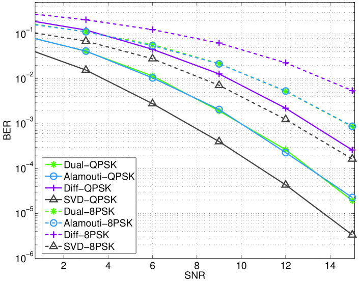
Figure 4: Performance comparison in $2\times 2$ MIMO systems: Dual Alamouti codes, Alamouti codes, differential transmission, and SVD methods.

First, we compare the dual Alamouti codes with the original Alamouti codes, differential transmission[5], and singular value decomposition (SVD) transmission using the largest eigen-direction. All schemes have a rate of one and achieve full spatial diversity for point-to-point MIMO systems. But the channel information requirements are different. The dual Alamouti codes need CSIT but no CSIR, while the original Alamouti codes need CSIR but no CSIT. For differential transmission, neither CSIT nor CSIR is required. The SVD scheme needs both CSIT and CSIR. Fig. 4 shows the simulated BER performance in a $2\times 2$ MIMO system with QPSK and 8PSK constellations. It can be observed that the dual Alamouti codes achieve the same BER as the original Alamouti codes. This can be confirmed by Proposition 1. The SVD scheme outperforms the other three transmission schemes due to its use of both CSIT and CSIR. The performance gap between the SVD scheme and the dual codes is approximately $2.5$ dB. Compared to the SVD scheme, the dual codes trade BER performance for less resources to learn CSIR.

Next, the proposed downlink IC schemes, with both equal and optimal power allocation, are compared with the BD methods using STBCs[22, 19] and an opportunistic TDMA scheme. Note that for a two-user $N\times 2$ BC, the BD method requires that the transmitter has at least four antennas. Alamouti codes are used on top of the ZF precoder to improve the diversity gain and reduce decoding complexity[22]. Such a BD method achieves 1 symbol/channel use/user and has the same symbol rate as the downlink IC scheme. Global CSIR is required at each receiver to decouple its two symbols carried in the Alamouti codes for each transmission. To compare with a TDMA scheme with CSIT and no CSIR, we propose an opportunistic TDMA scheme that assigns orthogonal time slots for each user and schedules the user with the stronger norm of channel coefficients to transmit using dual Alamouti codes. The opportunistic TDMA scheme has averagely only $0.5$ symbol/channel use/user, and a higher-order constellation is needed to compensate the rate loss. Also, it requires a longer decoding delay compared to both concurrent transmission schemes.

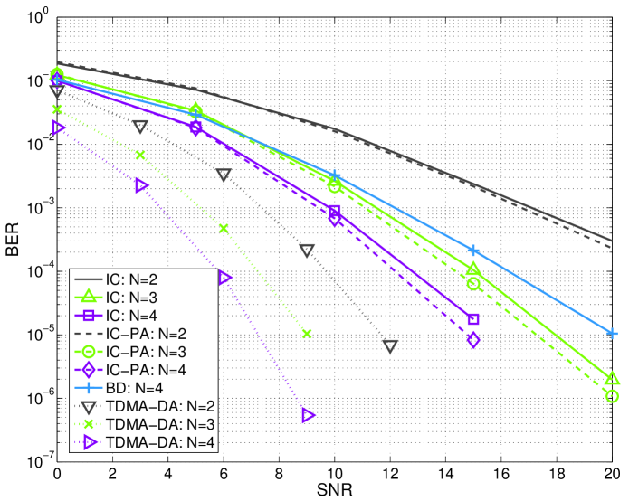
Figure 5: Performance comparison in two-user $N\times 2$ BC systems at $1$ bit/channel use/user: Downlink IC scheme (labeled as ‘IC’), Downlink IC scheme using optimal power allocation (labeled as ‘IC-PA’), BD methods, and opportunistic TDMA using dual Alamouti codes (labeled as ‘TDMA-DA’).

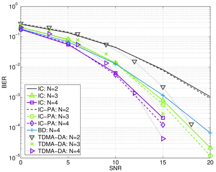
Figure 6: Performance comparison in two-user $N\times 2$ MIMO systems at $2$ bits/channel use/user: Downlink IC scheme (labeled as ‘IC’), Downlink IC scheme using optimal power allocation (labeled as ‘IC-PA’), BD methods, and opportunistic TDMA using dual Alamouti codes (labeled as ‘TDMA-DA’).

Figs. 5 and 6 exhibit the BER performance at rate=$1$ bit/channel user/user and rate=$2$ bits/channel use/user, respectively. In Fig. 5, BPSK is used for the downlink IC schemes and the BD methods, and QPSK for the opportunistic TDMA scheme; in Fig. 6, the downlink IC schemes and the BD methods use QPSK modulations, and the opportunistic TDMA scheme uses a 16-QAM constellation. We first compare the downlink IC scheme using equal power allocation with its optimal power allocation. From both figures, there is approximately $1$ dB array gain improvement for $N=3$ and $N=4$. The improvement for $N=2$ is about $0.5$ dB. The observation is consistent with Theorem 1 that power allocation improves the array gain but not the diversity gain. Next, we compare the downlink IC scheme with the BD method. From Figs. 5 and 6, the downlink IC scheme with $N=4$ outperforms the BD method with $N=4$ in the entire simulated SNR regime. Also with $N=3$, the downlink IC scheme outperforms the BD method with $N=4$ for SNR $>10$ dB. It can be observed that the proposed downlink IC scheme achieves a higher diversity gain compared to the BD method.

Finally, we compare the downlink IC scheme with our opportunistic TDMA scheme. In Fig. 5, the opportunistic TDMA scheme has substantial gain over the downlink IC scheme: the opportunistic TDMA scheme with $N=2$ can outperform the downlink IC scheme with $N=4$. This is because the opportunistic TDMA scheme exploits the multiuser diversity gain of $2N\times 2=4N$. It also explains the gains in Fig. 6 for SNR$>11$ dB. On the other hand, it can be observed in Fig. 6 that for $N=3$ and $N=4$, the downlink IC scheme has approximately $1$ dB gain over the opportunistic TDMA scheme for SNR$<10$ dB. The improvement is because the downlink IC scheme has a higher symbol rate compared to the opportunistic TDMA scheme.

V Conclusions

This paper investigates designs of communication systems with CSIT and no CSIR. We show such scenarios arise for concurrent transmissions in BC systems when users do not know the channels of other users. A duality principle has been proposed for systems with ZF designs. The duality principle connects the systems that know CSIR but not CSIT with the systems that know CSIT but not CSIR. We show an example to construct the dual system of the Alamouti codes, and propose the dual Alamouti codes for point-to-point MIMO systems. For the two-user downlink MIMO BC, we consider an IC scheme for the uplink MAC as the original system, and derive its downlink dual system, called the downlink IC scheme. The transmitter uses CSIT to design linear precoders and each receiver cancels interference and decouples its own data streams using two linear operations independent of CSIR. Power allocation between two users are also discussed. For a two-user $N\times 2$ BC, the downlink IC schemes achieve a diversity gain of $2(N-1)$ at rate $1$ symbol/channel use/user with both equal and optimal power allocations. The proposed schemes trade higher diversity for rate compared to the full-rate BD scheme. Simulation results demonstrate their superior BER performance over the BD methods concatenated with STBCs, which require global CSIR at each receiver.

Appendices

V-A Proof of Proposition 2

We prove this proposition for User $1$ only. Since the network is symmetrical, i.e., the user indices can be exchanged, similar results can be obtained for User $2$. We first show that the signals of User $2$ is zero-forced at User $1$. Since the $2\times 2(N-1)$ matrix $\mathbf{E}^{(k)}$ has the same structure as $\mathbf{F}^{(k)}$, the $2\times 2$ submatrices of $\mathbf{E}^{(k)}$ also have Alamouti structures. Then, $\tilde{\mathbf{X}}^{(k)}$ in (109) is composed of $2\times 2$ matrices with Alamouti structures due to the completeness of Alamouti structures under multiplication. We can represent $\tilde{\mathbf{X}}^{(k)}$ by

$$\tilde{\mathbf{X}}^{(k)}=\left[\begin{array}[]{ccccc}\tilde{x}_{11}^{(k)}&\tilde{x}_{21}^{(k)}&\cdots&\tilde{x}_{1(N-1)}^{(k)}&\tilde{x}_{2(N-1)}^{(k)}\\ -\tilde{x}_{21}^{(k)*}&\tilde{x}_{11}^{(k)*}&\cdots&-\tilde{x}_{2(N-1)}^{(k)*}&\tilde{x}_{1(N-1)}^{(k)*}\end{array}\right],k\in\{1,2\}.$$ (132)

The received signals $r_{11}^{(1)}$ and $r_{22}^{(1)}$ can be expanded as

$${r}_{11}^{(1)}=\sqrt{\frac{P}{2}}\sum_{k}\underset{\tilde{\mathbf{x}}^{(k)}}{\underbrace{\left[\begin{array}[]{c}\tilde{x}_{11}^{(k)}\\ \tilde{x}_{21}^{(k)}\\ \vdots\\ \tilde{x}_{1(N-1)}^{(k)}\\ \tilde{x}_{2(N-1)}^{(k)}\end{array}\right]^{\mathrm{T}}}}\left[\begin{array}[]{cccc}\frac{h_{11}^{(\underline{k})*}}{\|{\mathbf{h}}_{1}^{(\underline{k})}\|^{2}}&0&\cdots&-\frac{h_{N1}^{(\underline{k})*}}{\|{\mathbf{h}}^{(\underline{k})}_{N}\|^{2}}\\ \frac{h_{12}^{(\underline{k})*}}{\|{\mathbf{h}}_{1}^{(\underline{k})}\|^{2}}&0&\cdots&-\frac{h_{N2}^{(\underline{k})*}}{\|{\mathbf{h}}^{(\underline{k})}_{N}\|^{2}}\\ \vdots&\ddots&\ddots&\vdots\\ 0&\cdots&\frac{h_{(N-1)1}^{(\underline{k})*}}{\|{\mathbf{h}}_{N-1}^{(\underline{k})}\|^{2}}&-\frac{h_{N1}^{(\underline{k})*}}{\|{\mathbf{h}}^{(\underline{k})}_{N}\|^{2}}\\ 0&\cdots&\frac{h_{(N-1)2}^{(\underline{k})*}}{\|{\mathbf{h}}_{N-1}^{(\underline{k})}\|^{2}}&-\frac{h_{N2}^{(\underline{k})*}}{\|{\mathbf{h}}^{(\underline{k})}_{N}\|^{2}}\end{array}\right]\left[\begin{array}[]{c}{h}_{11}^{(1)}\\ h_{21}^{(1)}\\ \vdots\\ h_{N1}^{(1)}\end{array}\right]+w_{11},$$

$${r}_{22}^{(1)*}=\sqrt{\frac{P}{2}}\sum_{k}\tilde{\mathbf{x}}^{(k)}\left[\begin{array}[]{cccc}\frac{h_{12}^{(\underline{k})}}{\|{\mathbf{h}}_{1}^{(\underline{k})}\|^{2}}&0&\cdots&-\frac{h_{N2}^{(\underline{k})}}{\|{\mathbf{h}}^{(\underline{k})}_{N}\|^{2}}\\ -\frac{h_{11}^{(\underline{k})}}{\|{\mathbf{h}}_{1}^{(\underline{k})}\|^{2}}&0&\cdots&\frac{h_{N1}^{(\underline{k})}}{\|{\mathbf{h}}^{(\underline{k})}_{N}\|^{2}}\\ \vdots&\ddots&\ddots&\vdots\\ 0&\cdots&\frac{h_{(N-1)2}^{(\underline{k})}}{\|{\mathbf{h}}_{N-1}^{(\underline{k})}\|^{2}}&-\frac{h_{N2}^{(\underline{k})}}{\|{\mathbf{h}}^{(\underline{k})}_{N}\|^{2}}\\ 0&\cdots&-\frac{h_{(N-1)1}^{(\underline{k})}}{\|{\mathbf{h}}_{N-1}^{(\underline{k})}\|^{2}}&\frac{h_{N1}^{(\underline{k})}}{\|{\mathbf{h}}^{(\underline{k})}_{N}\|^{2}}\end{array}\right]\left[\begin{array}[]{c}{h}_{12}^{(1)*}\\ h_{22}^{(1)*}\\ \vdots\\ h_{N2}^{(1)*}\end{array}\right]+w_{22}^{*}.$$

Denote $\bar{\mathbf{h}}^{(1)}=\left[h_{11}^{(1)}\ -h_{12}^{(1)*}\ \cdots\ h_{N1}^{(1)}\ -h_{N2}^{(1)*}\right]^{\mathrm{T}}$ and

$$\tilde{\mathbf{H}}_{i}^{(\underline{k})}=\left[\begin{array}[]{cc}h_{i1}^{(\underline{k})}&h_{i2}^{(\underline{k})}\\ -h_{i2}^{(\underline{k})*}&h_{i1}^{(\underline{k})*}\end{array}\right],$$ (135)

which has an Alamouti structure. It follows that

$$\bar{r}_{1}^{(1)}=r_{11}^{(1)}+r_{22}^{(1)*}=\sqrt{\frac{P}{2}}\sum_{k}\tilde{\mathbf{x}}^{(k)}\tilde{\mathbf{B}}^{(\underline{k})}\bar{\mathbf{h}}^{(1)}+w_{11}^{(1)}+w_{22}^{(1)*},$$ (136)

where the $2(N-1)\times 2N$ matrix $\tilde{\mathbf{B}}^{(\underline{k})}$ has the same structure as the ZF matrix $\bar{\mathbf{Z}}^{(k)}$ in (99) and replaces each $2\times 2$ matrix $\frac{2\tilde{\mathbf{G}}_{i}^{(k)*}}{\|\tilde{\mathbf{G}}_{i}^{(k)}\|^{2}}$ with $\frac{\tilde{\mathbf{H}}_{i}^{(\underline{k})}}{\|\mathbf{h}_{i}^{(\underline{k})}\|^{2}}$ for $i=1,\ldots,N$. Further let $\tilde{\mathbf{h}}^{(1)}=\left[h_{12}^{(1)}\ h_{11}^{(1)*}\ \cdots\ h_{N2}^{(1)}\ h_{N1}^{(1)*}\right]^{\mathrm{T}}$. Similarly, we have $\bar{r}_{2}^{(1)}=r_{12}^{(1)}-r_{21}^{(1)*}=\sqrt{\frac{P}{2}}\underset{k}{\sum}\tilde{\mathbf{x}}^{(k)}\tilde{\mathbf{B}}^{(\underline{k})}\tilde{\mathbf{h}}^{(1)}+w_{12}^{(1)}-w_{21}^{(1)*}.$ Combine these two equations as,

$$\left[\begin{array}[]{cc}\bar{r}_{1}^{(1)}&\bar{r}_{2}^{(1)}\end{array}\right] =\sqrt{\frac{P}{2}}\sum_{k}\tilde{\mathbf{x}}^{(k)}\tilde{\mathbf{B}}^{(\underline{k})}\underset{\tilde{\mathbf{H}}^{(1)}}{\underbrace{\left[\bar{\mathbf{h}}^{(1)}\ \tilde{\mathbf{h}}^{(1)}\right]}}+\mathbf{w}^{(1)}=\sqrt{\frac{P}{2}}\tilde{\mathbf{x}}^{(1)}\tilde{\mathbf{B}}^{(2)}\tilde{\mathbf{H}}^{(1)}+\mathbf{w}^{(1)},$$ (138)

where $\mathbf{w}^{(1)}$ denotes the equivalent $1\times 2$ noise vector

$$\mathbf{w}^{(1)}=\left[\begin{array}[]{cc}w_{11}^{(1)}+w_{22}^{(1)*}&w_{12}^{(1)}-w_{21}^{(1)*}\end{array}\right].$$ (140)

Note that $\tilde{\mathbf{H}}^{(1)}=\left[\tilde{\mathbf{H}}_{1}^{(1)*}\ \cdots\ \tilde{\mathbf{H}}_{N}^{(1)*}\right]^{*}$, whose $2\times 2$ submatrice denotes the equivalent Alamouti channel matrix from Antenna $i$. The signal of User $1$ is cancelled because $\tilde{\mathbf{B}}^{(2)}$ zero-forces $\tilde{\mathbf{H}}^{(1)}$.

In what follows, we show that the symbols $s_{1}^{(1)}$ and $s_{2}^{(1)}$ are decoupled. From the structure of the symbol separating filter, we have $\tilde{\mathbf{x}}^{(1)}=\left[s_{1}^{(1)}\ s_{2}^{(1)}\right]\mathbf{E}^{(1)}$. Note that $\mathbf{E}^{(1)}$ has the same structure as $\mathbf{F}^{(1)}$ but replacing $g_{ji}^{(\kappa)}$ with $h_{ij}^{(\kappa)}$ for $\kappa\in\{1,2\}$. From (103), we have

$$\mathbf{E}^{(1)}=\beta^{(1)}\left(\tilde{\mathbf{B}}^{(2)}\tilde{\mathbf{H}}^{(1)}\right)^{*}$$ (141)

where $\beta^{(1)}=\frac{\sqrt{2}}{\|\tilde{\mathbf{H}}^{(1)*}\tilde{\mathbf{B}}^{(2)*}\tilde{\mathbf{B}}^{(2)}\|}$. Eq. (138) can be further written as

$$\left[\begin{array}[]{c}\bar{r}_{1}^{(1)}\\ \bar{r}_{2}^{(1)}\end{array}\right]^{\mathrm{T}} =\sqrt{\frac{P}{2}}\left[\begin{array}[]{c}s_{1}^{(1)}\\ s_{2}^{(1)}\end{array}\right]^{\mathrm{T}}\beta^{(1)}\left(\tilde{\mathbf{B}}^{(2)}\tilde{\mathbf{H}}^{(1)}\right)^{*}\tilde{\mathbf{B}}^{(2)}\tilde{\mathbf{H}}^{(1)}+\mathbf{w}^{(1)}=\sqrt{\frac{P}{2}}\frac{\beta^{(1)}}{2}\left[\begin{array}[]{c}s_{1}^{(1)}\\ s_{2}^{(1)}\end{array}\right]^{\mathrm{T}}\|\tilde{\mathbf{B}}^{(2)}\tilde{\mathbf{H}}^{(1)}\|^{2}+\mathbf{w}^{(1)}.$$

The second equality is achieved because the $2\times 2$ submatrices of $\tilde{\mathbf{B}}^{(2)}\tilde{\mathbf{H}}^{(1)}$ have Alamouti structures.

V-B Proof of Theorem 1

When the system uses an equal-energy constellation, the ML decoding can be conducted without CSIR. Then, the diversity gain performance depends only on the output instantaneous receive SNR. A method analyzing the diversity gain based on instantaneous receive SNR is presented in [26]. The techniques in [26] focus on the first-order exponent of the outage probability of the instantaneous receive SNR. For equal power allocation with $c_{k}=1$, the resulting SNR can be rewritten as $\mathrm{SNR}^{(k)}=\frac{Pb_{k}}{8}$ from (127). Note that $b_{k}$ has the same expression as the instantaneous normalized receive SNR of the uplink IC scheme that achieves a diversity gain of $2(N-1)$[25]. Thus, with equal power allocation, the downlink IC scheme also achieves a diversity gain of $2(N-1)$.

When power is distributed to maximize the smaller of the output SNRs at each user, the resulting SNR can be expressed as $\mathrm{SNR}^{(k)}=\frac{Pb_{1}b_{2}}{4(b_{1}+b_{2})}$. From the definition of the optimization problem in (128), we always have $\frac{Pb_{1}b_{2}}{4(b_{1}+b_{2})}\geq\min\left(\frac{Pb_{1}}{8},\frac{Pb_{2}}{8}\right)$. Further, because of the inequality $\frac{b_{1}b_{2}}{b_{1}+b_{2}}\leq\frac{b_{1}b_{2}}{b_{k}}=b_{\underline{k}}$, we can obtain $\frac{Pb_{1}b_{2}}{4(b_{1}+b_{2})}\leq\frac{P}{4}\min\left(b_{1},b_{2}\right)$. It follows that $\frac{P}{8}\min\left(b_{1},b_{2}\right)\leq\mathrm{SNR}^{(k)}\leq\frac{P}{4}\min\left(b_{1},b_{2}\right).$ This implies that $\mathrm{SNR}^{(k)}$ scales with $P\min\left(b_{1},b_{2}\right)$. Note that both $b_{1}$ and $b_{2}$ have diversity gain $2(N-1)$. Then, $\min\left(b_{1},b_{2}\right)$ also has diversity gain $2(N-1)$. Therefore, the system with optimal power allocation achieves diversity gain $2(N-1)$.

TABLE I: Classification of multi-antenna communication systems with respect to the channel information

Category	CSIT	CSIR	References
System A	No	No	[3, 4, 5]
System B	No	Yes	[6, 7]
System C	Yes	Yes	[8, 9]
System D	Yes	No

Figure 1: System diagram for two real systems. They are dual to each other under ZF designs.

Figure 2: Interference cancellation for the two-user uplink MAC.

Figure 3: Interference cancellation for the two-user downlink BC.

References

• [1] T. Marzetta and B. Hochwald, “Fast transfer of channel state information in wireless systems,” IEEE Transactions on Signal Processing, vol. 54, no. 4, pp. 1268 – 1278, Apr. 2006.
• [2] H. Jafarkhani, Space-Time Coding: Theory and Practice.   Cambridge University Press, 2005.
• [3] B. Hughes, “Differential space-time modulation,” IEEE Transactions on Information Theory, vol. 46, no. 7, pp. 2567 –2578, Nov. 2000.
• [4] B. Hochwald and W. Sweldens, “Differential unitary space-time modulation,” IEEE Transactions on Communications, vol. 48, no. 12, pp. 2041 –2051, Dec. 2000.
• [5] V. Tarokh and H. Jafarkhani, “A differential detection scheme for transmit diversity,” IEEE Journal on Selected Areas in Communications, vol. 18, no. 7, pp. 1169 –1174, Jul. 2000.
• [6] S. Alamouti, “A simple transmitter diversity scheme for wireless communications,” IEEE Journal on Selected Areas in Communications, vol. 16, pp. 1451 – 1458, Oct. 1998.
• [7] V. Tarokh, H. Jafarkhani, and A. Calderbank, “Space-time block codes from orthogonal designs,” IEEE Transactions on Information Theory, vol. 45, pp. 1456–1467, Jul. 1999.
• [8] G. Jongren, M. Skoglund, and B. Ottersten, “Combining beamforming and orthogonal space-time block coding,” IEEE Transactions on Information Theory, vol. 48, no. 3, pp. 611 –627, Mar. 2002.
• [9] S. Zhou and G. Giannakis, “Optimal transmitter eigen-beamforming and space-time block coding based on channel mean feedback,” IEEE Transactions on Signal Processing, vol. 50, no. 10, pp. 2599 – 2613, Oct. 2002.
• [10] P. Viswanath and D. Tse, “Sum capacity of the vector gaussian broadcast channel and uplink-downlink duality,” IEEE Transactions on Information Theory, vol. 49, no. 8, pp. 1912 – 1921, Aug. 2003.
• [11] S. Vishwanath, N. Jindal, and A. Goldsmith, “Duality, achievable rates, and sum-rate capacity of gaussian MIMO broadcast channels,” IEEE Transactions on Information Theory, vol. 49, no. 10, pp. 2658 – 2668, Oct. 2003.
• [12] H. Weingarten, Y. Steinberg, and S. Shamai, “The capacity region of the gaussian multiple-input multiple-output broadcast channel,” IEEE Transactions on Information Theory, vol. 52, no. 9, pp. 3936 –3964, Sep. 2006.
• [13] M. Costa, “Writing on dirty paper,” IEEE Transactions on Information Theory, vol. 29, no. 3, pp. 439 – 441, May 1983.
• [14] Q. Spencer, A. Swindlehurst, and M. Haardt, “Zero-forcing methods for downlink spatial multiplexing in multiuser MIMO channels,” IEEE Transactions on Signal Processing, vol. 52, no. 2, pp. 461 – 471, Feb. 2004.
• [15] Z. Shen, R. Chen, J. Andrews, R. Heath, and B. Evans, “Sum capacity of multiuser MIMO broadcast channels with block diagonalization,” IEEE Transactions on Wireless Communications, vol. 6, no. 6, pp. 2040 –2045, Jun. 2007.
• [16] H. Sung, S. Lee, and I. Lee, “Generalized channel inversion methods for multiuser MIMO systems,” IEEE Transactions on Communications, vol. 57, no. 11, pp. 3489 –3499, Nov. 2009.
• [17] T. Yoo, N. Jindal, and A. Goldsmith, “Multi-antenna downlink channels with limited feedback and user selection,” IEEE Journal on Selected Areas in Communications, vol. 25, no. 7, pp. 1478 –1491, Sep. 2007.
• [18] B. Khoshnevis and W. Yu, “A limited-feedback scheduling and beamforming scheme for multi-user multi-antenna systems,” in Proceedings of Globecom, Houston, Texas, Dec 2011.
• [19] D. Lee and K. Kim, “Reliability comparison of opportunistic scheduling and BD-precoding in downlink MIMO systems with multiple users,” IEEE Transactions on Wireless Communications, vol. 9, no. 3, pp. 964 –969, March 2010.
• [20] A. Naguib, N. Seshadri, and A. Calderbank, “Applications of space-time block codes and interference suppression for high capacity and high data rate wireless systems,” in Proc. of Asilomar Conf., Pacific Grove, CA, Oct. 1998.
• [21] A. Stamoulis, N. Al-Dhahir, and A. Calderbank, “Further results on interference cancellation and space-time block codes,” in Proc. of Asilomar Conf., Pacific Grove, CA, Oct. 2001.
• [22] R. Chen, J. Andrews, and R. Heath, “Multiuser space-time block coded MIMO with downlink precoding,” in 2004 IEEE International Conference on Communications, vol. 5, Jun. 2004, pp. 2689 – 2693.
• [23] L. Li and H. Jafarkhani, “Dual Alamouti codes,” in Proc. of IEEE Globecom 2011, Houston, Tx, Dec. 2011.
• [24] ——, “Short-term performance limits of MIMO systems with side information at the transmitter,” Technical report, available at http://arxiv.org/abs/1106.0733, Jun. 2011.
• [25] J. Kazemitabar and H. Jafarkhani, “Performance analysis of multiple-antenna multi-user detection,” Information Theory and Applications Workshop, Jan. 2009.
• [26] L. Li, Y. Jing, and H. Jafarkhani, “Using instantaneous normalized receive SNR for diversity gain calculation,” CPCC Technical Report, available at http://escholarship.org/uc/item/9511q6pf, Sep. 2010.