Abstract

The expectation-maximization (EM) algorithm is a powerful computational technique for finding the maximum likelihood estimates for parametric models when the data are not fully observed. The EM is best suited for situations where the expectation in each E-step and the maximization in each M-step are straightforward. A difficulty with the implementation of the EM algorithm is that each E-step requires the integration of the log-likelihood function in closed form. The explicit integration can be avoided by using what is known as the Monte Carlo EM (MCEM) algorithm. The MCEM uses a random sample to estimate the integral at each E-step. However, the problem with the MCEM is that it often converges to the integral quite slowly and the convergence behavior can also be unstable, which causes a computational burden. In this paper, we propose what we refer to as the quantile variant of the EM (QEM) algorithm. We prove that the proposed QEM method has an accuracy of $O(1/K^{2})$ while the MCEM method has an accuracy of $O_{p}(1/\sqrt{K})$. Thus, the proposed QEM method possesses faster and more stable convergence properties when compared with the MCEM algorithm. The improved performance is illustrated through the numerical studies. Several practical examples illustrating its use in interval-censored data problems are also provided.

Keywords: EM algorithm, incomplete data, maximum likelihood, MCEM, missing data, quantile

1 Introduction

The analysis of lifetime or failure time data has been of considerable interest in many branches of applied engineering statistics including reliability engineering, biological sciences, etc. In reliability analysis, due to inherent limitations, or time and cost considerations on experiments. The data are said to be censored when, for certain observations, only a lower or upper bound on the lifetime is available. Thus, there is partial information in the data set that still can be used in estimation for reliability analysis. To obtain the parameter estimate, numerical optimization is often required to find the MLE. However, ordinary numerical methods such as the Gauss-Seidel iterative method and the Newton-Raphson gradient method may be very ineffective for complicated likelihood functions and these methods can be sensitive to the choice of starting values used. In this paper, unless otherwise specified, “MLE” refers to the estimate obtained by direct maximization of the likelihood function.

For censored sample problems, several approximations of the MLE and the best linear unbiased estimate (BLUE) have been studied instead of direct calculation of the MLE. For example, the problem of parameter estimation from censored samples has been treated by several authors. Gupta¹ has studied the MLE and provided the BLUE for Type-I and Type-II censored samples from a normal distribution. Govindarajulu² has derived the BLUE for a symmetrically Type-II censored sample from a Laplace distribution only for sample size up to $n=20$. Balakrishnan³ has given an approximation of the MLE of the scale parameter of the Rayleigh distribution with censoring. Hassanein et al.⁴ also has given a BLUE for a Type-II censored sample from Rayleigh distribution. This BLUE, however, is limited to the case where the sample sizes are $n=5(1)25(5)45$ and the numbers of censored observations are $r=0,1,\ldots,n-2$, see Appendix F of Elsayed.⁵ Sultan⁶ has given an approximation of the MLE for a Type-II censored sample from a normal distribution. Balakrishnan⁷ has given the BLUE for a Type-II censored sample from a Laplace distribution. The BLUE needs the coefficients $a_{i}$ and $b_{i}$, which were tabulated in Balakrishnan,⁷ but the table is provided only for sample size up to $n=20$. In addition, the approximate MLE and the BLUE is not guaranteed to converge to the preferred MLE. The methods above are also restricted to Type-I or Type-II (symmetric) censoring for sample size up to $n=20$ only.

The previously mentioned deficiencies can be overcome through the use of the EM algorithm. However, in many practical problems, the implementation of the ordinary EM algorithm is very difficult because the expectation of the log-likelihood in the E-step can be quite complex or unavailable in closed form. In order to avoid the explicit construction of the expectation in the E-step, Wei and Tanner^{8, 9} proposed the use of the Monte Carlo EM (MCEM) algorithm when the E-step is intractable. The MCEM algorithm uses Monte Carlo random sampling from the conditional distribution in order to construct an empirical estimate of the expected log-likelihood. However, the MCEM algorithm often presents difficulties because the convergence to the expected likelihood can often be slow and unstable. Therefore, we propose a quantile variant of the EM (QEM) algorithm that constructs the empirical estimate of the expected log-likelihood by non-random quantiles. The proposed variant is shown to have much faster convergence behavior and greater stability than the MCEM while at the same time requiring smaller sample sizes.

Moreover, in many experiments, more general incomplete observations are often encountered along with the fully observed data, where incompleteness arises due to right-censoring, left-censoring, grouping, quantal responses, etc. A general type of incomplete observations is of interval form. That is, a lifetime of a subject $X_{i}$ is specified as $a_{i}\leq X_{i}\leq b_{i}$. We deal with computing the MLE for this general form of incomplete data using the EM algorithm and its variants, the MCEM and QEM algorithms. This interval form can handle right-censoring, left-censoring, quantal responses and fully-observed observations. This proposed method can also handle the data from intermittent inspection which are referred to as grouped data. In the grouped data case, only the number of failures in each inspection period are provided. For example, the articles^{10, 11} provide an example using grouped data but they approximate the MLE and only consider the case where the lifetimes are exponentially distributed. Nelson¹² considers the maximum likelihood for grouped data but uses ordinary numerical methods which, as mentioned earlier, can often be problematic. The attractiveness of our proposed method is that it allows one to obtain the MLE using the QEM sequences under a variety of distributional assumptions. We will illustrate that it is easily applied to the cases described above and also provides more accurate estimates.

2 The EM and MCEM algorithms

In this section, we give a brief introduction of the EM and MCEM algorithms. Introduced by Dempster et al.,¹³ the EM algorithm is a powerful computational technique for finding the MLE of parametric models when there is no closed-form MLE, or the data are incomplete. For more details about this EM algorithm, good references are Little and Rubin,¹⁴ Tanner,¹⁵ Schafer,¹⁶ and Hunter and Lange.¹⁷

When the closed-form MLE from the likelihood function is not available, numerical methods are required to find the maximizer (i.e., MLE). However, ordinary numerical methods such as the Gauss-Seidel iterative method and the Newton-Raphson gradient method may be very ineffective for complicated likelihood functions and these methods can be sensitive to the choice of starting values used. In particular, if the likelihood function is flat near its maximum, the methods will stop before reaching the maximum. These potential problems can be overcome by using the EM algorithm.

The EM algorithm consists of two iterative steps: (i) the expectation step (E-step) and (ii) the maximization step (M-step). The advantage of the EM algorithm is that it solves a difficult incomplete-data problem by constructing two relatively straightforward steps. The E-step of each iteration computes the conditional expectation of the log-likelihood with respect to the incomplete data given the observed data. The M-step of each iteration then obtains the maximizer of the expected log-likelihood constructed in the E-step. Thus, the EM sequences repeatedly maximize the log-likelihood function of the complete data given the incomplete data instead of maximizing the potentially complicated likelihood function of the incomplete data directly. An additional advantage of this method compared to other direct optimization techniques is that it is very simple and it converges reliably. In general, if it converges, it converges to a local maximum. Hence, in the case of the unimodal and concave likelihood function, the EM sequences converge to the global maximizer from any starting value. We can employ this methodology for parameter estimation for interval-censored data because interval-censored data models are special cases of incomplete (missing) data models.

Here, we give a brief introduction of the EM and MCEM algorithms. Denote the vector of unknown parameters by ${\boldsymbol{\theta}}=(\theta_{1},\ldots,\theta_{p})$. Then the complete-data likelihood is

$$L^{c}({\boldsymbol{\theta}}|{\mathbf{x}})=\prod_{i=1}^{n}f(x_{i}),$$

where $\mathbf{x}=(x_{1},\ldots,x_{n})$ and we denote the observed part of $\mathbf{x}$ by ${\mathbf{y}}=(y_{1},\ldots,y_{m})$ and the incomplete (missing) part by ${\mathbf{z}}=(z_{m+1},\ldots,z_{n})$. Denote the estimate at the $s$-th EM sequences by ${\boldsymbol{\theta}}^{(s)}$. The EM algorithm consists of two distinct steps:

• E-step: Compute $Q({\boldsymbol{\theta}}|{\boldsymbol{\theta}}^{(s)})$
  where $Q({\boldsymbol{\theta}}|{\boldsymbol{\theta}}^{(s)})=\int\log L^{c}({\boldsymbol{\theta}}|{\mathbf{y,z}})\,p({\mathbf{z}}|{\mathbf{y}},{\boldsymbol{\theta}}^{(s)})d{\mathbf{z}}$.

  
  

• M-step: Find ${\boldsymbol{\theta}}^{(s+1)}$
  which maximizes $Q({\boldsymbol{\theta}}|{\boldsymbol{\theta}}^{(s)})$ with respect to ${\boldsymbol{\theta}}$.

As stated earlier, the implementation of the E-step in the EM algorithm can sometimes be quite difficult. In order to avoid this difficulty, Wei and Tanner^{8, 9} proposed the MCEM algorithm. In the MCEM, the expected log-likelihood in the E-step is approximated by using Monte Carlo integration. By simulating $z_{m+1},\ldots,z_{n}$ from the conditional distribution $p({\mathbf{z}}|{\mathbf{y}},{\boldsymbol{\theta}}^{(s)})$, the MCEM approximates the expected log-likelihood in the E-step. Let $K$ denote the number of samples used in the Monte Carlo integration of the MCEM and denote each simulated sample by ${\mathbf{z}}^{(k)}=(z_{m+1,k},\ldots,z_{n,k})$. Then the Monte Carlo approximation of the expected log-likelihood is

$$\widehat{Q}({\boldsymbol{\theta}}|{\boldsymbol{\theta}}^{(s)})=\frac{1}{K}\sum_{k=1}^{K}\log L^{c}({\boldsymbol{\theta}}|{\mathbf{y}},{\mathbf{z}}^{(k)}).$$ (1)

This method where the E-step is changed to create an empirical estimate of the expected log-likelihood is called the MCEM algorithm. Unfortunately, the major drawback to the MCEM algorithm is that it can often be very slow because it requires a large sample size for the empirical estimate to converge to the expected likelihood. In addition, the values of the parameter estimation during each run of the MCEM algorithm can vary because random samples are used in the Monte Carlo integration. In fact, the dependence of the MCEM algorithm on random sampling implies that, even when using a large number of iterations, two identical runs of the MCEM algorithm can result in different parameter estimates. These issues that arise due to the dependence of the MCEM algorithm on random sampling are avoided in the QEM algorithm through the use of deterministic sequences. In fact, random sampling is completely avoided in the QEM.

3 The quantile variant of the EM algorithm

The key idea underlying the QEM algorithm can be easily illustrated by the following example. The data set in the example was first presented by Freireich et al.¹⁸ and has since then been used very frequently for illustration in the reliability engineering and survival analysis literature.^{19, 20, 21}

3.1 Illustrative example: length of remission of leukemia patients

An experiment is conducted to determine the effect of a drug named 6-mercaptopurine (6-MP) on leukemia remission times. Twenty-one leukemia patients ($n=21$) are treated with 6-MP and the times of remission are recorded. There are nine individuals ($m=9$) for whom the remission time is fully observed, and the remission times for the remaining twelve individuals are randomly censored on the right. Letting a plus (+) denote a censored observation, the remission times (in weeks) are: 6, 6, 6, $6^{+}$, 7, $9^{+}$, 10, $10^{+}$, $11^{+}$, 13, 16, $17^{+}$, $19^{+}$, $20^{+}$, 22, 23, $25^{+}$, $32^{+}$, $32^{+}$, $34^{+}$, $35^{+}$.

Assuming an exponential distribution for the lifetimes with the probability density function (pdf)

$$f(x)=\frac{1}{\theta}e^{-x/\theta},$$

we obtain the complete likelihood function

$$\log L^{c}({\theta}|{\mathbf{y,z}}) =-n\log\theta-\frac{1}{\theta}\sum_{i=1}^{m}y_{i}-\frac{1}{\theta}\sum_{i=m+1}^{n}z_{i}$$

and the conditional pdf

$$p({\mathbf{z}}|{\mathbf{y}},{\theta}^{(s)},R_{i}) =\prod_{i=m+1}^{n}p_{z_{i}}(z_{i}|\theta^{(s)},R_{i})$$

$$=\prod_{i=m+1}^{n}\frac{1}{\theta^{(s)}}e^{-(z_{i}-R_{i})/\theta^{(s)}},$$

where $z_{i}>R_{i}$ and $R_{i}$ is a right-censoring time of the $i$-th test unit. Using the above conditional pdf, we have the expected log-likelihood

$$Q({\theta}|{\theta}^{(s)})$$

$$=\int\log L^{c}(\theta|{\mathbf{y,z}})\;p({\mathbf{z}}|{\mathbf{y}},{\theta}^{(s)},R_{i})d{\mathbf{z}}$$

$$=-n\log\theta-\frac{1}{\theta}\sum_{i=1}^{m}y_{i}-\frac{1}{\theta}\sum_{i=m+1}^{n}\int z_{i}\;p_{z_{i}}(z_{i}|\theta^{(s)},R_{i})dz_{i}$$

$$=-n\log\theta-(n-m)\frac{\theta^{(s)}}{\theta}-\frac{1}{\theta}\sum_{i=1}^{m}y_{i}-\frac{1}{\theta}\sum_{i=m+1}^{n}R_{i}.$$

In the Monte Carlo approximation, the term

$$E[z_{i}|\theta^{(s)}]=\int z_{i}p_{z_{i}}(z_{i}|\theta^{(s)},R_{i})dz_{i}$$

is approximated by

$$E[z_{i}|\theta^{(s)}]=\int z_{i}p_{z_{i}}(z_{i}|\theta^{(s)},R_{i})dz_{i}\approx\frac{1}{K}\sum_{k=1}^{K}z_{i,k},$$ (2)

where a random sample $z_{i,k}$ is from

$$p_{z_{i}}(z_{i}|\theta^{(s)},R_{i})=\frac{1}{\theta^{(s)}}e^{-(z_{i}-R_{i})/\theta^{(s)}}.$$

Then the Monte Carlo approximation of the expected log-likelihood is given by

$$\widehat{Q}({\theta}|{\theta}^{(s)})=-n\log\theta-\frac{1}{\theta}\sum_{i=1}^{m}y_{i}-\frac{1}{\theta}\frac{1}{K}\sum_{k=1}^{K}\sum_{i=m+1}^{n}z_{i,k}.$$

Figure 1: The expected log-likelihood functions and approximations. (a) Monte Carlo approximations. (b) Quantile approximations.

The key idea behind the QEM is that the approximation above can be improved by using the quantile function. Given the conditional pdf $p_{z_{i}}(z_{i,k}|\theta^{(s)},R_{i})$, we denote the quantiles of $\xi_{k}$ as

$$q_{i,k}=F^{-1}(\xi_{k}|\theta^{(s)},R_{i})=R_{i}-\theta^{(s)}\log(1-\xi_{k}).$$ (3)

One can choose $\xi_{k}$ from any form of the deterministic sequences such as $k/K$, $k/(K+1)$, $(k-\frac{1}{2})/K$, etc. In this paper, we use $\xi_{k}=(k-\frac{1}{2})/K$ for $k=1,2,\ldots,K$. By analogy with equation (2), we can approximate the term

$$E[z_{i}|\theta^{(s)}]=\int z_{i}p_{z_{i}}(z_{i}|\theta^{(s)},R_{i})dz_{i}.$$

Using the above quantiles $q_{i,k}$ in equation (3) instead of a random sample $z_{i,k}$, we have the following approximation

$$E[z_{i}|\theta^{(s)}]=\int z_{i}p_{z_{i}}(z_{i}|\theta^{(s)},R_{i})dz_{i}\approx\frac{1}{K}\sum_{k=1}^{K}q_{i,k}.$$ (4)

It is noteworthy that a random sample $z_{i,k}$ in the Monte Carlo approximation can be generated by using the inverse transform algorithm.²² That is, the quantiles of a uniform random sample generate a random sample $z_{i,k}$. However, the QEM uses the quantiles of the deterministic sequences $\xi_{k}=(k-\frac{1}{2})/K$ which ensure faster and more stable convergence properties when compared with the MCEM.

Figure 1 presents the MCEM and QEM approximations of the expected log-likelihood functions for $K=10$ (dashed curve), 100 (dotted curve) and 1,000 (dot-dashed curve) at the first step ($s=1$), along with the exact expected log-likelihood (solid curve). The MCEM and QEM algorithms were run with starting value $\theta^{(0)}=1$. As can be seen in Figure 1, the MCEM and QEM both successfully converge to the expected log-likelihood as $K$ gets larger. Note that the QEM is much closer to the true expected log-likelihood for smaller values of $K$. As afore-mentioned, it should be noted again that estimates based on the MCEM can produce different values dependent on a random sample. Thus, the curves in Figure 1 (a) can change for each different random sample. On the other hand, the curves in Figure 1 (b) do not change because the QEM uses the deterministic sequences $\xi_{k}=(k-\frac{1}{2})/K$.

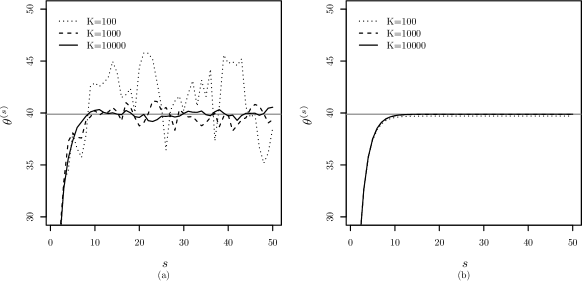
Figure 2: Successive parameter estimates using (a) the MCEM and (b) the QEM. The horizontal solid lines indicate the MLE ($\hat{\theta}=39.89$).

The plots of the parameter estimates at each value of $s$ for the MCEM and QEM are shown in Figures 2 (a) and (b) respectively with the horizontal lines indicating the MLE ($\hat{\theta}=39.89$). We used the starting value with $\theta^{(0)}=1$. The figures clearly show that convergence behavior of the QEM is quite stable and the number of steps required for convergence of the QEM is much smaller than that of the MCEM. For example, using $K=100$ in the QEM results in faster convergence than using $K=10,000$ in the MCEM.

3.2 Convergence properties of the MCEM and QEM algorithms

The two key questions are why the QEM is more stable and more accurate than the MCEM. Both of the questions can be answered by considering the approximation in equation (4) as an approximation to a Riemann-Stieltjes integral. For simplicity of presentation, we only consider the case where ${\mathbf{z}}$ is one-dimensional but the same argument can be used in the case where ${\mathbf{z}}$ is multivariate. Denote $h({\theta},z)=\log L^{c}(\theta|{\mathbf{y}},z)$ and consider the following Riemann-Stieltjes sum

$$\frac{1}{K}\sum_{k=1}^{K}h(\theta,F^{-1}\big{(}\xi_{k}\big{)}).$$ (5)

Note that in the limit as $K\to\infty$, we have

$$\frac{1}{K}\sum_{k=1}^{K}h(\theta,F^{-1}\big{(}\xi_{k}\big{)})\longrightarrow\int_{0}^{1}h(\theta,F^{-1}(\xi))d\xi.$$ (6)

Using a change-of-variable integration technique with $z=F^{-1}(\xi)$, we have

$$\int h(\theta,z)dF(z)=\int h(\theta,z)f(z)dz.$$

Notice that the quantile approximation on the left-hand side of (6) is a Riemann-Stieltjes sum which converges to the integral on the right-hand side of (6). In our specific case, the integral represents the expected log-likelihood which therefore proves that the QEM converges.

The next step is to show why the QEM has better accuracy when compared with the MCEM. With $\xi_{k}=(k-\frac{1}{2})/K$, the sum in equation (5) is also known as the extended midpoint rule which is well known to possess accuracy to the order of $O(1/K^{2})$.²³ Specifically, it can be easily shown that

$$\int h(\theta,z)f(z)dz=\frac{1}{K}\sum_{k=1}^{K}h({\boldsymbol{\theta}},q_{k})+O\Big{(}\frac{1}{K^{2}}\Big{)},$$ (7)

where $q_{k}=F^{-1}(\xi_{k})$. Thus, the accuracy of the integration in the E-step of the QEM is $O(1/K^{2})$.

On the other hand, the accuracy of the Monte Carlo approximation

$$\overline{h}_{K}=\frac{1}{K}\sum_{k=1}^{K}h(\theta,z_{k})$$

can be assessed as follows. By the central limit theorem, we have

$$\frac{\sqrt{K}\Big{\{}\overline{h}_{K}-E(h(\theta,z))\Big{\}}}{\sqrt{{\mathrm{Var}}(h(\theta,z))}}\stackrel{{\scriptstyle d}}{{\longrightarrow}}N(0,1)$$ (8)

which is accurate to the order of $O_{p}(1)$. Using the weak law of large numbers, we have

$$\overline{h}_{K}\stackrel{{\scriptstyle p}}{{\longrightarrow}}E(h(\theta,z)).$$

Using this along with equation (8) results in

$$\int h(\theta,z)f(z)dz=\frac{1}{K}\sum_{k=1}^{K}h(\theta,z_{k})+O_{p}\Big{(}\frac{1}{\sqrt{K}}\Big{)}.$$ (9)

Note that we have shown that the E-step of the QEM has accuracy of deterministic $O(1/K^{2})$ and the E-step of the MCEM has accuracy of probabilistic $O_{p}(1/\sqrt{K})$. Therefore, the QEM has faster and more stable convergence properties compared to those of the MCEM.

We can generalize the above result as follows. In the E-step, using the quantiles instead of random samples, we replace the Monte Carlo approximation of the expected log-likelihood in equation (1) with the following quantile approximation

$$\widehat{Q}(\theta|{\theta}^{(s)})=\frac{1}{K}\sum_{k=1}^{K}\log L^{c}(\theta|{\mathbf{y}},{\mathbf{q}}^{(k)}),$$

where $\log L^{c}(\cdot)$ is the complete-data log-likelihood in the EM algorithm, ${\mathbf{q}}^{(k)}=(q_{m+1,k},\ldots,q_{n,k})$ with $q_{i,k}=F^{-1}_{z_{i}}(\xi_{k}|{\theta}^{(s)})$, and we used $\xi_{k}=(k-\frac{1}{2})/K$ as afore-mentioned.

Note that the approximation of the expected log-likelihood in the proposed QEM method can be viewed as being similar to a quasi-Monte Carlo approximation in the sense that the quasi-Monte Carlo approximation also uses deterministic sequences rather than a random sample. In fact, Niederreiter²⁴ shows that there exist such sequences in the normalized integration domain, which ensure accuracy on the order of $O(K^{-1}(\log K)^{d-1})$, where $d$ is the dimension of the integration space.²⁵ Thus, using the quasi-Monte Carlo sequences in the normalized integration domain, one can improve the accuracy of the integration in the E-step of the MCEM algorithm which leads to accuracy to the order of $O(1/K^{1})$ with $d=1$. However, we should point out that the proposed QEM method leads to accuracy to the order of $O(1/K^{2})$. Therefore, although using the quasi-Monte Carlo approximation can improve the convergence properties of the MCEM, the accuracy in that case will still be less than that of the proposed QEM method. Also, incorporating the quantiles from the proposed QEM method into the M-step to obtain the MLE is quite straightforward. Note also that, if the quasi-Monte Carlo sequences in the normalized integration domain are used, this operation will not have any relevance in the M-step in the sense that it still may be quite difficult to obtain a closed-form solution for the maximization.

Another way to approximate the expected log-likelihood is the use of a direct numerical integration in the E-step. For example, instead of using the approximation

$$E[z_{i}|\theta^{(s)}] =\int z_{i}\,p_{z_{i}}(z_{i}|\theta^{(s)},R_{i})dz_{i}$$

$$\approx(1/K)\sum_{k=1}^{K}z_{i,k}$$

in equation (2), one may use

$$E[z_{i}|\theta^{(s)}] =\int z_{i}\,p_{z_{i}}(z_{i}|\theta^{(s)},R_{i})dz_{i}$$

$$\approx\sum_{k=1}^{K}t_{i,k}\,p_{z_{i}}(t_{i}|\theta^{(s)},R_{i})\Delta t_{i}$$

where $\Delta t_{i}=t_{i,k}-t_{i,k-1}$, $t_{i,0}=a_{i}$ (the lower bound of the support of $z_{i}$), and $t_{i,K}=b_{i}$ (upper bound). However, if the above direct numerical integration is used instead of the MCEM approximation $(1/K)\sum_{k=1}^{K}z_{i,k}$ or the QEM approximation $(1/K)\sum_{k=1}^{K}q_{i,k}$, this can create a problem in the M-step because this direct numerical integration includes the pdf term $p_{z_{i}}(t_{i}|\theta^{(s)},R_{i})$ in the sum. Thus, the integral becomes much more complex and this complexity can make it difficult or even impossible to find the closed-form maximizer in the M-step. It should also be noted that the integrating domain of a direct numerical integration is the same as the support of a random variable while the integrating domain of the QEM method is always between zero and one as shown in equation (6). If the support of a random variable is unbounded as is often the case in statistics, a numerical integration of an improper integral should be used; see Section 4.4 of Press et al.²³ Improper integrals present serious challenges in numerical integration. In order to obtain reasonable accuracy using numerical integration, great care needs to be taken and often advanced methods need to be used. Thus, the focus of the paper is to construct the EM algorithm using the quantiles so that the closed-form maximizer in the M-step can be obtained in a straightforward manner.

4 Likelihood construction

In this section, we develop the likelihood functions which can be conveniently used for the EM, MCEM and QEM algorithms.

The general form of an incomplete observation is often of interval form. That is, the lifetime of a subject $X_{i}$ may not be observed exactly, but is known to fall in an interval, $a_{i}\leq X_{i}\leq b_{i}$. This interval form includes censored, grouped, quantal-response, and fully-observed observations. For example, a lifetime is left-censored when $a_{i}=-\infty$ and a lifetime is right-censored when $b_{i}=\infty$. The lifetime is fully observed when $a_{i}=b_{i}$.

Suppose that ${\mathbf{x}}=(x_{1},\ldots,x_{n})$ are observations on random variables which are independent and identically distributed (iid) and have a continuous distribution with pdf $f(x)$ and cumulative distribution function (cdf) $F(x)$. Interval-censored data from experiments can be conveniently represented by pairs $(w_{i},\delta_{i})$ with $w_{i}=[a_{i},b_{i}]$,

$$\delta_{i}=\left\{\begin{array}[]{r@{\quad\mathrm{if}~}l}0\quad\mathrm{if}~&a_{i}<b_{i}\\ 1\quad\mathrm{if}~&a_{i}=b_{i}\end{array}\right.\qquad{\mathrm{for}}\quad i=1,\ldots,n,$$

where $\delta_{i}$ is an indicator variable and $a_{i}$ and $b_{i}$ are lower and upper ends of interval observations of the $i$-th test unit, respectively. If $a_{i}=b_{i}$, then the lifetime of the $i$-th test unit is fully observed. Denote the observed part of $\mathbf{x}=(x_{1},\ldots,x_{n})$ by ${\mathbf{y}}=(y_{1},\ldots,y_{m})$ and the incomplete (missing) part by ${\mathbf{z}}=(z_{m+1},\ldots,z_{n})$ with $a_{i}\leq z_{i}\leq b_{i}$. Denote the vector of unknown parameters by ${\boldsymbol{\theta}}=(\theta_{1},\ldots,\theta_{d})$. Then ignoring a normalizing constant, we have the complete-data likelihood function

$${L}^{c}({\boldsymbol{\theta}}|{\mathbf{y,z}})\propto\prod_{i=1}^{n}f(x_{i}|{\boldsymbol{\theta}})=\prod_{i=1}^{m}f(y_{i}|{\boldsymbol{\theta}})\cdot\prod_{i=m+1}^{n}f(z_{i}|{\boldsymbol{\theta}}),$$ (10)

where the pdf of $z_{i}$ is given by

$$p_{z_{i}}(z|{\boldsymbol{\theta}})=\frac{f(z|{\boldsymbol{\theta}})}{F(b_{i}|{\boldsymbol{\theta}})-F(a_{i}|{\boldsymbol{\theta}})},$$ (11)

for $a_{i}<z<b_{i}$.

Integrating ${L}^{c}({\boldsymbol{\theta}}|{\mathbf{x}})$ with respect to ${\mathbf{z}}$, we obtain the observed-data likelihood

$${L}({\boldsymbol{\theta}}|{\mathbf{y}}) \propto\int{L}^{c}({\boldsymbol{\theta}}|{\mathbf{y,z}})d{\mathbf{z}}$$

$$=\prod_{i=1}^{m}f(y_{i}|{\boldsymbol{\theta}})\prod_{i=m+1}^{n}\big{\{}F(b_{i}|{\boldsymbol{\theta}})-F(a_{i}|{\boldsymbol{\theta}})\big{\}},$$

where an empty product is generally taken to be one. Using the $(w_{i},\delta_{i})$ notation, we have

$${L}({\boldsymbol{\theta}}|{\mathbf{w}},{\boldsymbol{\delta}})\propto\prod_{i=1}^{n}f(w_{i}|{\boldsymbol{\theta}})^{\delta_{i}}\big{\{}F(b_{i}|{\boldsymbol{\theta}})-F(a_{i}|{\boldsymbol{\theta}})\big{\}}^{1-\delta_{i}},$$ (12)

where ${\mathbf{w}}=(w_{1},\ldots,w_{n})$ and ${\boldsymbol{\delta}}=(\delta_{1},\ldots,\delta_{n})$. Here, although we provided the likelihood function for the interval-data case, it is easily extended to more general forms of incomplete data. For more details, the reader is referred to Heitjan²⁶ and Heitjan and Rubin.²⁷

Clearly, given the complexity of the likelihood, the goal is to make an inference on ${\boldsymbol{\theta}}$ and the EM algorithm is a tool that can be used to accomplish this goal. Then the issue here is how to implement the EM algorithm when there are interval-censored data in the sample. By treating the interval-censored data as incomplete (missing) data, it is possible to write the complete-data likelihood. This treatment allows one to fine the closed-form maximizer in the M-step. For convenience, assume that all the data are of interval form with $a_{i}\leq w_{i}\leq b_{i}$ and $a_{i}<b_{i}$. Then the likelihood function in equation (12) can be rewritten as

$${L}({\boldsymbol{\theta}}|{\mathbf{w}})\propto\prod_{i=1}^{n}\big{\{}F(b_{i}|{\boldsymbol{\theta}})-F(a_{i}|{\boldsymbol{\theta}})\big{\}}.$$ (13)

Then the complete-data likelihood function corresponding to equation (13) is given by

$${L}^{c}({\boldsymbol{\theta}}|{\mathbf{y}},{\mathbf{z}})\propto\prod_{i=1}^{n}f(z_{i}|{\boldsymbol{\theta}}),$$

where the pdf of $z_{i}$ is given by equation (11). Using this result, we have the following $Q$-function in the E-step:

$$Q({\boldsymbol{\theta}}|{\boldsymbol{\theta}}^{(s)})=\sum_{i=1}^{n}\int_{a_{i}}^{b_{i}}\log f(z_{i}|\boldsymbol{\theta})\cdot p_{z_{i}}(z_{i}|{\boldsymbol{\theta}^{(s)}})\,dz_{i}.$$

It is useful to consider the integral above when $b_{i}\to a_{i}$. For notational convenience, omitting the subject index $i$ and letting $b=a+\epsilon$, we have

$$\int_{a}^{a+\epsilon}\log f(z|\boldsymbol{\theta})\cdot p_{z}(z|{\boldsymbol{\theta}^{(s)}})\,dz.$$ (14)

It follows from integration by parts that the integral above becomes

$$\Big{[}\log f(z|\boldsymbol{\theta})P_{z}(z|{\boldsymbol{\theta}^{(s)}})\Big{]}_{a}^{a+\epsilon}\!\!\!-\int_{a}^{a+\epsilon}\frac{f^{\prime}(z|\boldsymbol{\theta})}{f(z|\boldsymbol{\theta})}P_{z}(z|{\boldsymbol{\theta}^{(s)}})\,dz,$$ (15)

where

$$P_{z}(z|{\boldsymbol{\theta}^{(s)}})=\frac{F(z|\boldsymbol{\theta}^{(s)})}{F(a+\epsilon|\boldsymbol{\theta}^{(s)})-F(a|\boldsymbol{\theta}^{(s)})}.$$ (16)

Using equations (15) and (16), we can rewrite (14) as

$$\frac{A-B-C}{F(a+\epsilon|\boldsymbol{\theta}^{(s)})-F(a|\boldsymbol{\theta}^{(s)})},$$ (17)

where

$$A =\log f(a+\epsilon|\boldsymbol{\theta})F(a+\epsilon|\boldsymbol{\theta}^{(s)}),$$

$$B =\log f(a|\boldsymbol{\theta})F(a|\boldsymbol{\theta}^{(s)}),$$

and

$$C =\int_{a}^{a+\epsilon}\frac{f^{\prime}(z|\boldsymbol{\theta})}{f(z|\boldsymbol{\theta})}\cdot F(z|{\boldsymbol{\theta}^{(s)}})\,dz.$$

Applying l’Hospital rule to equation (17), we obtain

$$\lim_{\epsilon\to 0}\int_{a}^{a+\epsilon}\log f(z|\boldsymbol{\theta})\cdot p_{z}(z|{\boldsymbol{\theta}^{(s)}})\,dz=\log f(a|{\boldsymbol{\theta}}).$$

Thus, in the case where all the lifetimes are fully observed, we simply use the interval $[a_{i},a_{i}]$ notation which implies $[a_{i},a_{i}+\epsilon]$ with the limit as $\epsilon\to 0^{+}$. Using this result, all the data points considered in this paper can be viewed as data points in interval-data form without requiring the use of the indicator variable $\delta_{i}$.

For notational convenience, we let $z_{1}=y_{1},\ldots,z_{m}=y_{m}$. Then the complete-data likelihood function corresponding to equation (10) becomes

$${L}^{c}({\boldsymbol{\theta}}|{\mathbf{z}})\propto\prod_{i=1}^{n}f(z_{i}|{\boldsymbol{\theta}}),$$ (18)

where ${\mathbf{z}}=(z_{1},z_{2},\ldots,z_{n})$. From now, unless otherwise specified, ${\mathbf{z}}$ refers to $(z_{1},z_{2},\ldots,z_{n})$ instead of $(z_{m+1},z_{2},\ldots,z_{n})$. Thus, we use equation (18) for the complete-data likelihood function rather than equation (10).

For many distributions, it is extremely difficult or even impossible to implement the EM algorithm with interval-censored data. This is because, in the E-step, the $Q$-function does not integrate easily and this causes computational difficulties in the M-step. In order to avoid this problem, one can use the MCEM algorithm which reduces the difficulty in the E-step through the use of a Monte Carlo integration. As aforementioned, although it can make some problems tractable, the MCEM can be computationally very expensive and often leads to unstable estimates. Thus, we propose a quantile variant of the EM algorithm, the QEM, which alleviates the computational issues associated with the MCEM algorithm and leads to more stable estimates.

Regardless of whether one uses EM, MCEM or QEM, a stopping criteria needs to be defined so that the algorithm converges after some number of iterations. We define the stopping criteria as one in which the changes in successive estimates are relatively small compared to a defined precision $\epsilon$. For example, in the case of the normal distribution, we can define the stopping criteria for the QEM algorithm to occur when both

$$\big{|}\mu^{(s+1)}-{\mu}^{(s)}\big{|}<\epsilon{\mu}^{(s+1)}$$

and

$$\big{|}\sigma^{(s+1)}-{\sigma}^{(s)}\big{|}<\epsilon{\sigma}^{(s+1)},$$

where $\epsilon$ is some small number which depends on one’s desired precision. For other convergence criteria, the reader may refer to Press et al.²³

In the section that follows, we maximize the likelihood function in equation (12) using the EM (when available), MCEM and QEM algorithms under a variety of distributional assumptions.

5 Parameter estimation

In this section, we provide examples of parameter estimation using the EM, MCEM and QEM algorithms under various distributional assumptions. Specifically, we consider the exponential, normal, Laplace, Rayleigh and Weibull distributions in turn.

In the case where the exponential and normal distributions are assumed, the implementation of the EM algorithm is straightforward and there is actually no need to consider the MCEM or the QEM algorithms. Nevertheless, in order to compare the performance of the MCEM and the QEM under those distributional assumptions, we include the results of these approaches also. Also, for the details involved in generating the EM sequences of the normal distribution with interval censoring, the readers are referred to Lee and Park.²⁸

Now, in the case where we assume that the lifetimes have a Laplace distribution, the E-step computation in the EM algorithm is extremely complex so the MCEM and QEM are more appropriate and we expect the QEM to outperform the MCEM. Finally, when the Rayleigh and Weibull distributions are assumed for the lifetimes, the expected log-likelihood in the E-step of the EM does not have an explicit integration so it is not possible to apply the EM algorithm in these cases.

As aforementioned, it is noteworthy that the QEM sequences are easily obtained by replacing a random sample ${\mathbf{z}}^{(k)}$ in the MCEM sequences with quantile sequences ${\mathbf{q}}^{(k)}$.

5.1 Exponential distribution

We assume that the random variables $z_{i}$ are iid exponential random variables with the pdf given by $f(z|\lambda)=\lambda\exp(-\lambda z)$. Using equation (18), we obtain the complete-data log-likelihood of ${\lambda}$

$$\log L^{c}(\lambda|\mathbf{z})=\sum_{i=1}^{n}(\log\lambda-\lambda z_{i}),$$

where the pdf of $z_{i}$ is given by

$$p_{z_{i}}(z|\lambda)=\frac{\lambda\exp(-\lambda z)}{\exp(-\lambda a_{i})-\exp(-\lambda b_{i})},$$ (19)

for $a_{i}<z<b_{i}$. When $a_{i}=b_{i}$, the above random variables $z_{i}$ degenerate at $z_{i}=a_{i}$.

• E-step:
  When $a_{i}<b_{i}$, the $Q(\cdot)$ function is given by

  $$Q(\lambda|\lambda^{(s)}) =\int\log L^{c}(\lambda|{\mathbf{z}})\,p({\mathbf{z}}|\lambda^{(s)})d{\mathbf{z}}$$

  $$=n\log\lambda-\lambda\sum_{i=1}^{n}A_{i}^{(s)},$$

  where

  $$p({\mathbf{z}}|\lambda^{(s)})=\prod_{i=1}^{n}p_{z_{i}}(z_{i}|\lambda^{(s)})$$

  and

  $$A_{i}^{(s)} =E[z_{i}|\lambda^{(s)}]=\int_{a_{i}}^{b_{i}}\!\!\!z\cdot p_{z_{i}}(z|\lambda^{(s)})\,dz$$

  $$=\frac{a_{i}\exp(-\lambda^{(s)}a_{i})-b_{i}\exp(-\lambda^{(s)}b_{i})}{\exp(-\lambda^{(s)}a_{i})-\exp(-\lambda^{(s)}b_{i})}+\frac{1}{\lambda^{(s)}}.$$

  Note that when $a_{i}=b_{i}$, we have $A_{i}^{(s)}=a_{i}$.

  
  

• M-step:
  Differentiating $Q(\lambda|\lambda^{(s)})$ with respect to $\lambda$ and setting this to zero, we obtain

  $$\frac{\partial Q(\lambda|\lambda^{(s)})}{\partial\lambda}=\frac{n}{\lambda}-\sum_{i=1}^{n}A_{i}^{(s)}=0.$$

  Solving for $\lambda$, we obtain the $(s+1)$st EM sequence in the M-step

  $$\lambda^{(s+1)}=\frac{n}{\sum_{i=1}^{n}A_{i}^{(s)}}.$$ (20)

If we instead use the MCEM algorithm by simulating $z_{1},\ldots,z_{n}$ from the truncated exponential distribution $p({\mathbf{z}}|{\boldsymbol{\theta}}^{(s)})$, we then obtain the MCEM sequences

$$\lambda^{(s+1)}=\frac{n}{\sum_{i=1}^{n}\frac{1}{K}\sum_{k=1}^{K}z_{i,k}},$$

where $z_{i,k}$ for $k=1,2,\ldots,K$ are from the truncated exponential distribution $p_{z_{i}}(z|\lambda^{(s)})$ defined in equation (19). On the other hand, if we use the QEM algorithm by quantiling, we then obtain the QEM sequences

$$\lambda^{(s+1)}=\frac{n}{\sum_{i=1}^{n}\frac{1}{K}\sum_{k=1}^{K}q_{i,k}},$$

where $q_{i,k}=F_{z_{i}}^{-1}(\xi_{k}|{\lambda}^{(s)})$ and $\xi_{k}=(k-\frac{1}{2})/K$. It is immediate from equation (19) that

$$F_{z_{i}}(z|\lambda)=\frac{\exp(-\lambda a_{i})-\exp(-\lambda z)}{\exp(-\lambda a_{i})-\exp(-\lambda b_{i})},$$

for $a_{i}<z<b_{i}$, $F_{z_{i}}(z|\lambda)=0$ for $z\leq a_{i}$, and $F_{z_{i}}(z|\lambda)=1$ for $z\geq b_{i}$. Thus, the quantile sequences are explicitly obtained as

$$q_{i,k} =\frac{1}{{\lambda}^{(s)}}\times$$

$$\qquad\log\Big{[}\frac{1}{(1-\xi_{k})\exp(-\lambda^{(s)}a_{i})+\xi_{k}\exp(-\lambda^{(s)}b_{i})}\Big{]}.$$

It is of interest to consider the case where the data are right-censored. In this special case, the closed-form MLE is known. If the data are fully observed (i.e., $w_{i}=[a_{i},a_{i}]$) for $i=1,2,\ldots,r$, it is easily seen from l’Hospital rule that $A_{i}^{(s)}=a_{i}$. If the observation is right-censored (i.e., $w_{i}=[a_{i},\infty]$) for $i=r+1,\ldots,n$, we have $A_{i}^{(s)}=a_{i}+1/\lambda^{(s)}$. Substituting these results into equation (20) leads to

$$\lambda^{(s+1)}=\frac{n}{\sum_{i=1}^{n}a_{i}+(n-r)/\lambda^{(s)}}.$$ (21)

Note that solving the stationary-point equation $\hat{\lambda}=\lambda^{(s+1)}=\lambda^{(s)}$ of equation (21) gives

$$\hat{\lambda}=\frac{r}{\sum_{i=1}^{n}a_{i}}.$$

As expected, the results is identical to the well-known closed-form MLE in the right-censored data case.

5.2 Normal distribution

We assume that the random variables $z_{i}$ are iid normal random variables with parameter vector $\boldsymbol{\theta}=(\mu,\sigma)$. Using equation (18), we obtain the complete-data log-likelihood of $\boldsymbol{\theta}$

$$\log L^{c}({\boldsymbol{\theta}}|\mathbf{z}) \propto-\frac{n}{2}\log\sigma^{2}-\frac{n}{2\sigma^{2}}\mu^{2}$$

$$\qquad-\frac{1}{2\sigma^{2}}\Big{\{}\sum_{i=1}^{n}\!z_{i}^{2}-2\mu\sum_{i=1}^{n}\!z_{i}\Big{\}},$$

where the pdf of $z_{i}$ is given by

$$p_{z_{i}}(z|{\boldsymbol{\theta}})=\frac{\frac{1}{\sigma}\phi(\frac{z-\mu}{\sigma})}{\Phi(\frac{b_{i}-\mu}{\sigma})-\Phi(\frac{a_{i}-\mu}{\sigma})},$$ (22)

for $a_{i}<z<b_{i}$. Similarly as before, if $a_{i}=b_{i}$, then the random variables $z_{i}$ degenerate at $z_{i}=a_{i}$.

• E-step:
  Denote the estimate of $\boldsymbol{\theta}$ at the $s$-th EM sequence by $\boldsymbol{\theta}^{(s)}=(\mu^{(s)},\sigma^{(s)})$. Ignoring constant terms, we have

  $$Q({\boldsymbol{\theta}}|{\boldsymbol{\theta}}^{(s)}) =\int\log L^{c}({\boldsymbol{\theta}}|{\mathbf{z}})\,p({\mathbf{z}}|{\boldsymbol{\theta}}^{(s)})d{\mathbf{z}}$$

  $$=-\frac{n}{2}\log\sigma^{2}-\frac{n}{2\sigma^{2}}\mu^{2}-\frac{1}{2\sigma^{2}}\sum_{i=1}^{n}A_{i}^{(s)}$$

  $$\qquad+\frac{\mu}{\sigma^{2}}\sum_{i=1}^{n}B_{i}^{(s)},$$

  where $p({\mathbf{z}}|{\boldsymbol{\theta}}^{(s)})=\prod_{i=1}^{n}p_{z_{i}}(z_{i}|{\boldsymbol{\theta}}^{(s)})$, $A_{i}^{(s)}=E[z_{i}^{2}|{\boldsymbol{\theta}}^{(s)}]$ and $B_{i}^{(s)}=E[z_{i}|{\boldsymbol{\theta}}^{(s)}]$. Using the following integral identities

  $$\int\frac{z}{\sigma}\phi(\frac{z-\mu}{\sigma})dz =\mu\Phi(\frac{z-\mu}{\sigma})-\sigma\phi(\frac{z-\mu}{\sigma})$$

  and

  $$\int\frac{z^{2}}{\sigma}\phi(\frac{z-\mu}{\sigma})dz =(\mu^{2}+\sigma^{2})\Phi(\frac{z-\mu}{\sigma})$$

  $$\qquad-\sigma(\mu+z)\phi(\frac{z-\mu}{\sigma}),$$

  we obtain

  $$A_{i}^{(s)} =\{\mu^{(s)}\}^{2}+\{\sigma^{(s)}\}^{2}-\sigma^{(s)}\times$$

  $$\frac{(\mu^{(s)}+b_{i})\phi(\frac{b_{i}-\mu^{(s)}}{\sigma^{(s)}})-(\mu^{(s)}+a_{i})\phi(\frac{a_{i}-\mu^{(s)}}{\sigma^{(s)}})}{\Phi(\frac{b_{i}-\mu^{(s)}}{\sigma^{(s)}})-\Phi(\frac{a_{i}-\mu^{(s)}}{\sigma^{(s)}})}$$

  and

  $$B_{i}^{(s)} =\mu^{(s)}-\sigma^{(s)}\times\frac{\phi(\frac{b_{i}-\mu^{(s)}}{\sigma^{(s)}})-\phi(\frac{a_{i}-\mu^{(s)}}{\sigma^{(s)}})}{\Phi(\frac{b_{i}-\mu^{(s)}}{\sigma^{(s)}})-\Phi(\frac{a_{i}-\mu^{(s)}}{\sigma^{(s)}})},$$

  where $a_{i}<b_{i}$. It should be noted that for $a_{i}=b_{i}$ we have $A_{i}^{(s)}=a_{i}^{2}$ and $B_{i}^{(s)}=a_{i}$.

  
  

• M-step:
  Differentiating the expected log-likelihood $Q({\boldsymbol{\theta}}|{\boldsymbol{\theta}}^{(s)})$ with respect to $\mu$ and $\sigma^{2}$ and solving for $\mu$ and $\sigma^{2}$, we obtain the EM sequences

  $$\mu^{(s+1)} =\frac{1}{n}\sum_{i=1}^{n}B_{i}^{(s)},$$ (23)

  and

  $${\sigma^{2}}^{(s+1)} =\frac{1}{n}\sum_{i=1}^{n}A_{i}^{(s)}-\big{\{}\mu^{(s+1)}\big{\}}^{2}.$$ (24)

If we instead use the MCEM algorithm by simulating $z_{1},\ldots,z_{n}$ from the truncated normal distribution $p({\mathbf{z}}|{\boldsymbol{\theta}}^{(s)})$, we then obtain the MCEM sequences

$$\mu^{(s+1)} =\frac{1}{n}\sum_{i=1}^{n}\frac{1}{K}\sum_{k=1}^{K}z_{i,k},$$ (25)

and

$${\sigma^{2}}^{(s+1)} =\frac{1}{n}\sum_{i=1}^{n}\frac{1}{K}\sum_{k=1}^{K}z_{i,k}^{2}-\big{\{}\mu^{(s+1)}\big{\}}^{2},$$ (26)

where $z_{i,k}$ are from the truncated normal distribution $p_{z_{i}}({z_{i,k}}|\mu^{(s)},\sigma^{(s)})$ defined in equation (22). Note that the QEM algorithm is easily obtained by quantiling $z_{1},\ldots,z_{n}$. As illustrated in the exponential case, the quantiles are easily obtained using $q_{i,k}=F^{-1}_{z_{i}}(\xi_{k}|\mu^{(s)},\sigma^{(s)})$. Thus, replacing $z_{i,k}$ in equations (25) and (26) with $q_{i,k}$, we can obtain the QEM sequences.

5.3 Laplace distribution

We assume that the random variables $z_{i}$ are iid Laplace random variables with parameter $\boldsymbol{\theta}=(\mu,\sigma)$ whose pdf is given by

$$f(x|\mu,\sigma)=\frac{1}{2\sigma}\exp\Big{(}-\frac{|x-\mu|}{\sigma}\Big{)}.$$

Using equation (18), we have the complete-data log-likelihood of $\boldsymbol{\theta}$

$$\log{L}^{c}({\boldsymbol{\theta}}|{\mathbf{z}}) =C-n\log\sigma-\frac{1}{\sigma}\sum_{i=1}^{m}|y_{i}-\mu|$$

$$\quad-\frac{1}{\sigma}\sum_{i=m+1}^{n}|z_{i}-\mu|,$$

where the pdf of $z_{i}$ is given by

$$p_{z_{i}}(z|\boldsymbol{\theta})=\frac{f(z|\boldsymbol{\theta})}{F(b_{i}|\boldsymbol{\theta})-F(a_{i}|\boldsymbol{\theta})}$$ (27)

for $a_{i}<z<b_{i}$. Similarly as before, if $a_{i}=b_{i}$, then the random variables $z_{i}$ degenerate at $z_{i}=a_{i}$.

• E-step:
  At the $s$-th step in the EM sequence denoted by ${\boldsymbol{\theta}}^{(s)}=(\mu^{(s)},\sigma^{(s)})$, we have the expected log-likelihood

  $$Q({\boldsymbol{\theta}}|{\boldsymbol{\theta}}^{(s)})$$

  $$=\int\log L^{c}({\boldsymbol{\theta}}|{\mathbf{z}})\,p({\mathbf{z}}|{\boldsymbol{\theta}}^{(s)})d{\mathbf{z}}$$

  $$=C-n\log\sigma-\frac{1}{\sigma}\sum_{i=1}^{n}\int_{a_{i}}^{b_{i}}|z_{i}-\mu|\,f({z_{i}}|{\boldsymbol{\theta}}^{(s)})d{z_{i}}.$$

  Note that integrating the third term in the expression above is extremely complex. We can avoid this difficulty by using the MCEM algorithm or the QEM algorithm. Using the standard MCEM technique given $K$ samples, the approximate expected log-likelihood becomes

  $$\widehat{Q}({\boldsymbol{\theta}}|{\boldsymbol{\theta}}^{(s)})$$

  $$=\frac{1}{K}\sum_{k=1}^{K}\log L^{c}({\boldsymbol{\theta}}|{\mathbf{z}}^{(k)})$$

  $$=C-n\log\sigma-\frac{1}{\sigma}\sum_{i=1}^{n}\frac{1}{K}\sum_{k=1}^{K}\big{|}z_{i,k}-\mu\big{|},$$ (28)

  where $\mathbf{z}^{(k)}=(z_{1,k},z_{2,k},\ldots,z_{n,k})$. Therefore, we can estimate the expected log-likelihood by generating $z_{i,k}$ for $k=1,2,\ldots,K$ from $p_{z_{i}}(z|{\boldsymbol{\theta}}^{(s)})$ defined in equation (27). Then by replacing $z_{i,k}$ in equation (28) with the quantiles $q_{i,k}=F^{-1}_{z_{i}}(\xi_{k}|\mu^{(s)},\sigma^{(s)})$, the E-step for the QEM algorithm is easily obtained.

  
  

• M-step:
  It is straightforward to obtain the MCEM and QEM sequences which maximize equation (28)

  $$\mu^{(s+1)} ={\mathrm{median}}({\mathbf{z}}^{(1)},\ldots,{\mathbf{z}}^{(K)})$$ (29)

  and

  $$\sigma^{(s+1)} =\frac{1}{n}\sum_{i=1}^{n}\frac{1}{K}\sum_{k=1}^{K}\big{|}z_{i,k}-\mu^{(s+1)}\big{|}.$$ (30)

  Again, replacing $z_{i,k}$ in equations (29) and (30) with the quantiles $q_{i,k}$ provides the QEM sequences.

Note that if the direct numerical integration is used instead of the MCEM or QEM approximation, the approximate expected log-likelihood becomes

$$\widehat{Q}({\boldsymbol{\theta}}|{\boldsymbol{\theta}}^{(s)})$$

$$=C-n\log\sigma-\frac{1}{\sigma}\sum_{i=1}^{n}\sum_{k=1}^{K}\big{|}t_{i,k}-\mu\big{|}f({t_{i,k}}|{\boldsymbol{\theta}}^{(s)})\Delta t_{i},$$ (31)

where $\Delta t_{i}=t_{i,k}-t_{i,k-1}$, $t_{i,0}=a_{i}$ and $t_{i,K}=b_{i}$. When this direct numerical integration is used, the terms, $f({t_{i,k}}|{\boldsymbol{\theta}}^{(s)})$ and $\Delta t_{i}$, are involved inside the sum in equation (31) and these are not constant. On the other hand, the QEM and MCEM algorithms do not include these $\Delta t_{i}=t_{i,k}-t_{i,k-1}$ terms. Therefore, it can be easily seen that the median of $t_{i,k}$ can not be the maximizer of equation (31) with respect to $\mu$. To the best of our knowledge, a closed-form maximizer for equation (31) does not exist. As mentioned earlier, the use of the direct numerical integration makes it very difficult or even impossible to find the closed-form maximizer in the M-step. The point to be made here is that direct numerical integration is not useful because it is still requires an intractable or at the very least, extremely difficult, maximization in the M-step. The advantage of MCEM and QEM over direct numerical integration is that they simplify the M-step considerably.

5.4 Rayleigh distribution

Let the random variables $z_{i}$ be iid Rayleigh random variables with parameter $\beta$ whose pdf is given by

$$f(z|\beta)=\frac{z}{\beta^{2}}\exp\big{(}-\frac{z^{2}}{2\beta^{2}}\big{)},\quad z>0,~{}\beta>0.$$

Using equation (18), we have the complete-data log-likelihood of $\beta$

$$\log L^{c}({{\beta}}|{\mathbf{z}}) =C-2n\log\beta+\sum_{i=1}^{n}\log z_{i}-\frac{1}{2\beta^{2}}\sum_{i=1}^{n}z_{i}^{2},$$

where the pdf of the random variable $z_{i}$ is given by

$$p_{z_{i}}(z|\beta)=\frac{\frac{z}{\beta^{2}}\exp\big{(}-\frac{z^{2}}{2\beta^{2}}\big{)}}{\exp\big{(}-\frac{a_{i}^{2}}{2\beta^{2}}\big{)}-\exp\big{(}-\frac{b_{i}^{2}}{2\beta^{2}}\big{)}}$$ (32)

for $a_{i}<z<b_{i}$. Similarly as before, if $a_{i}=b_{i}$, then the random variables $z_{i}$ degenerate at $z_{i}=a_{i}$.

• E-step:
  At the $s$-th step in the EM sequence denoted by $\beta^{(s)}$, we have the expected log-likelihood

  $$Q(\beta|\beta^{(s)})$$

  $$\quad=\int\log L^{c}(\beta|{\mathbf{z}})p({\mathbf{z}}|\beta^{(s)})d{\mathbf{z}}$$

  $$\quad=C-2n\log\beta$$

  $$\qquad+\sum_{i=1}^{n}\int_{a_{i}}^{b_{i}}(\log z_{i}-\frac{1}{2\beta^{2}}z_{i}^{2})p_{z_{i}}({z_{i}}|\beta^{(s)})d{z_{i}}.$$

  The calculation of the above integration part does not have a closed form. Using the MCEM, we have the approximate expected log-likelihood

  $$\widehat{Q}({{\beta}}|{{\beta}}^{(s)}) =\frac{1}{K}\sum_{k=1}^{K}\log L^{c}({{\beta}}|{\mathbf{z}}^{(k)})$$

  $$=C-2n\log\beta+\frac{1}{K}\sum_{k=1}^{K}\sum_{i=1}^{n}\log z_{i,k}$$

  $$\qquad-\frac{1}{2\beta^{2}}\frac{1}{K}\sum_{k=1}^{K}\sum_{i=1}^{n}z_{i,k}^{2},$$

  where ${\mathbf{z}}^{(k)}=(z_{1,k},\ldots,z_{n,k})$ and $z_{i,k}$ for $k=1,2,\ldots,K$ are from $p_{z_{i}}(z|{\beta}^{(s)})$ defined in equation (32).

  
  

• M-step:
  We then obtain the following MCEM (or QEM) sequences by differentiating $\widehat{Q}({{\beta}}|{{\beta}}^{(s)})$

  $$\beta^{(s+1)}=\sqrt{\frac{1}{2n}\sum_{i=1}^{n}\frac{1}{K}\sum_{k=1}^{K}z_{i,k}^{2}}.$$ (33)

In the above, if the quantiles $q_{i,k}$ are used instead of a random sample $z_{i,k}$, then the QEM sequences are obtained.

5.5 Weibull distribution

We assume that $X_{i}$ are iid Weibull random variables with the pdf and cdf given by $f(x)=\lambda\beta x^{\beta-1}\exp(-\lambda x^{\beta})$ and $F(x)=1-\exp(-\lambda x^{\beta})$, respectively.

Using equation (18), we obtain the complete-data log-likelihood of $\boldsymbol{\theta}=(\lambda,\beta)$

$$\log L^{c}(\boldsymbol{\theta})=\sum_{i=1}^{n}\Big{\{}\log\lambda+\log\beta+(\beta-1)\log z_{i}-\lambda z_{i}^{\beta}\Big{\}},$$

where the pdf of $z_{i}$ is given by

$$p_{z_{i}}(z|\boldsymbol{\theta})=\frac{\lambda\beta z^{\beta-1}\exp(-\lambda z^{\beta})}{\exp(-\lambda a_{i}^{\beta})-\exp(-\lambda b_{i}^{\beta})},$$ (34)

for $a_{i}<z<b_{i}$. Similarly as before, if $a_{i}=b_{i}$, then the random variables $z_{i}$ degenerate at $z_{i}=a_{i}$.

• E-step:
  Denote the estimate of $\boldsymbol{\theta}$ at the $s$-th EM sequence by $\boldsymbol{\theta}^{(s)}=(\lambda^{(s)},\beta^{(s)})$. It follows from $Q(\boldsymbol{\theta}|\boldsymbol{\theta}^{(s)})=E\big{[}\log L^{c}(\boldsymbol{\theta})\big{]}$ that

  $$Q(\boldsymbol{\theta}|\boldsymbol{\theta}^{(s)}) =n\log\lambda+n\log\beta+(\beta-1)\sum_{i=1}^{n}A_{i}^{(s)}$$

  $$\qquad-\lambda\sum_{i=1}^{n}B_{i}^{(s)},$$

  where $A_{i}^{(s)}=E\big{[}\log z_{i}|\boldsymbol{\theta}^{(s)}\big{]}$ and $B_{i}^{(s)}=E\big{[}z_{i}^{\beta}|\boldsymbol{\theta}^{(s)}\big{]}$.

  
  

• M-step:
  Differentiating $Q(\lambda|\lambda^{(s)})$ with respect to $\lambda$ and $\beta$ and setting this to zero, we obtain

  $$\frac{\partial Q(\boldsymbol{\theta}|\boldsymbol{\theta}^{(s)})}{\partial\lambda} =\frac{n}{\lambda}-\sum_{i=1}^{n}B_{i}^{(s)}(\beta)=0$$ (35)

  and

  $$\frac{\partial Q(\boldsymbol{\theta}|\boldsymbol{\theta}^{(s)})}{\partial\beta} =\frac{n}{\beta}+\sum_{i=1}^{n}A_{i}^{(s)}-\lambda\sum_{i=1}^{n}\frac{\partial B_{i}^{(s)}(\beta)}{\partial\beta}=0.$$ (36)

  Solving equation (35) for $\lambda$ and substituting this $\lambda$ into equation (36), we obtain the following expression involving $\beta$

  $$\frac{1}{\beta}+\frac{1}{n}\sum_{i=1}^{n}A_{i}^{(s)}-\frac{\sum_{i=1}^{n}\frac{\partial B_{i}^{(s)}(\beta)}{\partial\beta}}{\sum_{i=1}^{n}B_{i}^{(s)}(\beta)}=0.$$

  Note that the $(s+1)$st element of EM sequence of $\beta$ is the solution of the equation above. Therefore, after finding $\beta^{(s+1)}$, we can then obtain the $(s+1)$st element of the EM sequence of $\lambda^{(s+1)}$

  $$\lambda^{(s+1)}=\frac{n}{\sum_{i=1}^{n}B_{i}^{(s)}(\beta^{(s+1)})}.$$

Note that, in the Weibull case, it is extremely difficult to obtain explicit expression for the expectations, $E\big{[}\log z_{i}|\boldsymbol{\theta}^{(s)}\big{]}$ and $E\big{[}z_{i}^{\beta}|\boldsymbol{\theta}^{(s)}\big{]}$ in the E-step. Fortunately, the quantile function of $z_{i}$ at the $s$-th step can be easily obtained, which makes the QEM particularly useful in the case of the Weibull assumption. Specifically, based on equation (34), we have

$$q_{i,k} =F^{-1}_{z_{i}}(\xi_{k}|\boldsymbol{\theta}^{(s)})$$

$$=\Bigg{[}-\frac{1}{\lambda^{(s)}}\log\Big{\{}(1-\xi_{k})\exp({-\lambda^{(s)}a_{i}^{\beta^{(s)}}})$$

$$\qquad\qquad+\xi_{k}\exp({-\lambda^{(s)}b_{i}^{\beta^{(s)}}})\Big{\}}\Bigg{]}^{1/\beta^{(s)}}.$$

Using the above quantiles, we obtain the following QEM algorithm.

• E-step:
  Denote the quantile approximation of $Q(\cdot)$ by $\widehat{Q}(\cdot)$. Then, we have

  $$\widehat{Q}(\boldsymbol{\theta}|\boldsymbol{\theta}^{(s)})=n\log\lambda+n\log\beta$$

  $$\quad+(\beta-1)\sum_{i=1}^{n}\frac{1}{K}\sum_{k=1}^{K}\log q_{i,k}-\lambda\sum_{i=1}^{n}\frac{1}{K}\sum_{k=1}^{K}q_{i,k}^{\beta}.$$

  
  

• M-step:
  Differentiating $\widehat{Q}(\lambda|\lambda^{(s)})$ with respect to $\lambda$ and $\beta$ and setting this to zero, we obtain

  $$\frac{\partial\widehat{Q}(\boldsymbol{\theta}|\boldsymbol{\theta}^{(s)})}{\partial\lambda} =\frac{n}{\lambda}-\frac{1}{K}\sum_{i=1}^{n}\sum_{k=1}^{K}q_{i,k}^{\beta}=0$$ (37)

  and

  $$\frac{\partial\widehat{Q}(\boldsymbol{\theta}|\boldsymbol{\theta}^{(s)})}{\partial\beta} =\frac{n}{\beta}+\frac{1}{K}\sum_{i=1}^{n}\sum_{k=1}^{K}\log q_{i,k}$$ (38)

  $$-\lambda\frac{1}{K}\sum_{i=1}^{n}\sum_{k=1}^{K}q_{i,k}^{\beta}\log q_{i,k}=0.$$ (39)

  Solving equation (37) for $\lambda$ and substituting this $\lambda$ into equation (39), we have the equation of $\beta$

  $$\frac{1}{\beta} +\frac{1}{nK}\sum_{i=1}^{n}\sum_{k=1}^{K}\log q_{i,k}$$

  $$-\frac{\sum_{i=1}^{n}\sum_{k=1}^{K}q_{i,k}^{\beta}\log q_{i,k}}{\sum_{i=1}^{n}\sum_{k=1}^{K}q_{i,k}^{\beta}}=0.$$ (40)

  Note that the $(s+1)$st element of QEM sequence of $\beta$ is the solution of the equation above. Therefore, after finding $\beta^{(s+1)}$, we can then obtain the $(s+1)$st element of the QEM sequence of $\lambda^{(s+1)}$

  $$\lambda^{(s+1)}=\frac{nK}{\sum_{i=1}^{n}\sum_{k=1}^{K}q_{i,k}^{\beta^{(s+1)}}}.$$

We should point out that, in the M-step, we need to estimate the shape parameter $\beta$ by solving equation (• ‣ 5.5) numerically. Note that upper and lower bounds for the root of equation (• ‣ 5.5) can be explicitly obtained. This implies that the solution can be obtained using only a one dimensional root search and the uniqueness of the solution is guaranteed. Under mild conditions, we provide a proof of the uniqueness in the appendix section along with the upper and lower bounds for $\beta$.

6 Simulation study

In order to examine the performance of the proposed QEM method, we carry out two different simulations. In the first simulation, we assume that the lifetimes are normally distributed. The second simulation assumes that the lifetimes have a Rayleigh distribution. The number of samples used for the MCEM and QEM algorithms was varied so that $K=10$, $10^{2}$, $10^{3}$, and $10^{4}$. The Monte Carlo simulations are based on $5,000$ replications. The Monte Carlo simulations are performed using the R language.²⁹

Table 1: Estimated biases and MSEs, and SREs of the EM, MCEM and QEM estimators assuming normally distributed data with $\mu=50$ and $\sigma=5$.

	$\hat{\mu}$
Method	Bias	MSE	SRE
EM	1.342988$\times 10^{-5}$	1.779955$\times 10^{-10}$	——
MCEM
$K=10$	7.169276$\times 10^{-2}$	8.381887$\times 10^{-3}$	2.123573$\times 10^{-8}$
$K=10^{2}$	2.223300$\times 10^{-2}$	8.170053$\times 10^{-4}$	2.178633$\times 10^{-7}$
$K=10^{3}$	7.135135$\times 10^{-3}$	8.417492$\times 10^{-5}$	2.114590$\times 10^{-6}$
$K=10^{4}$	2.265630$\times 10^{-3}$	8.433365$\times 10^{-6}$	2.110610$\times 10^{-5}$
QEM
$K=10$	2.511190$\times 10^{-2}$	2.558357$\times 10^{-5}$	6.957412$\times 10^{-6}$
$K=10^{2}$	2.382535$\times 10^{-3}$	2.305853$\times 10^{-7}$	7.719289$\times 10^{-4}$
$K=10^{3}$	2.349116$\times 10^{-4}$	2.432084$\times 10^{-9}$	7.318639$\times 10^{-2}$
$K=10^{4}$	3.232357$\times 10^{-5}$	2.176558$\times 10^{-10}$	8.177841$\times 10^{-1}$
	$\hat{\sigma}$
Method	Bias	MSE	SRE
EM	3.706033$\times 10^{-5}$	1.143094$\times 10^{-10}$	——
MCEM
$K=10$	1.139404$\times 10^{-1}$	2.133204$\times 10^{-2}$	5.358577$\times 10^{-9}$
$K=10^{2}$	3.540433$\times 10^{-2}$	2.069714$\times 10^{-3}$	5.522955$\times 10^{-8}$
$K=10^{3}$	1.137090$\times 10^{-2}$	2.130881$\times 10^{-4}$	5.364419$\times 10^{-7}$
$K=10^{4}$	3.621140$\times 10^{-3}$	2.150602$\times 10^{-5}$	5.315227$\times 10^{-6}$
QEM
$K=10$	5.580507$\times 10^{-2}$	1.272262$\times 10^{-4}$	8.984739$\times 10^{-7}$
$K=10^{2}$	5.890585$\times 10^{-3}$	1.418158$\times 10^{-6}$	8.060413$\times 10^{-5}$
$K=10^{3}$	6.315578$\times 10^{-4}$	1.644996$\times 10^{-8}$	6.948917$\times 10^{-3}$
$K=10^{4}$	9.699447$\times 10^{-5}$	4.529568$\times 10^{-10}$	2.523627$\times 10^{-1}$

We illustrate the performance of the proposed method with the EM and MCEM estimators by computing the respective mean biases and mean square errors (MSEs). The bias is defined as the sample average of the differences between the estimates under consideration and the MLE. The MLE is obtained by solving the log-likelihood estimating equation numerically using the nlm() function in R. The MSE is defined as the sample average of the squares of the differences between the estimates under consideration and the MLE.

Note that in order to compare the efficiency of the MCEM algorithm and QEM algorithms, we used an equal and fixed number of iterations in both simulations. In this manner, we compare the accuracy when the computational burden of each algorithm is the same. Both algorithms were stopped after ten iterations ($s=10$) and the simulation results are shown in Tables 1 and 2. Rather than fixing the number of iterations, we could have taken the alternative route of using the same stopping criteria for both the QEM and MCEM algorithms. Clearly, if the QEM accuracy is greater with the iterations being fixed, then a stopping criteria methodology would lead to similar accuracy but a greater number of iterations would be required for the MCEM stopping criteria to be triggered. So, the two comparison methodologies are, for all intents and purposes, equivalent and we chose the methodology in which the number of iterations are fixed to the same pre-determined value for both the MCEM and the QEM.

In the first simulation, a random sample of size $n=20$ was generated from the normal distribution with $\mu=50$ and $\sigma=5$. Also, the largest five data points from the sample were assumed to be right-censored. In order to compare the MCEM and QEM algorithms with the EM algorithm as a reference, a univariate statistical dispersion measure based on the MSE can be used to compare algorithm efficiency. Analogous to the relative efficiency,^{30, 31, 32} the simulated relative efficiency (SRE) is defined as

$$\mathrm{SRE}=\frac{\mathrm{simulated~{}MSE~{}of~{}the~{}EM~{}estimator}}{\mathrm{simulated~{}MSE~{}under~{}consideration}}.$$

Table 2: Estimated biases and MSEs of the MCEM and QEM estimators assuming Rayleigh distributed data with $\beta=10$.

		$\hat{\beta}$
Method		Bias	MSE
MCEM
$K=10$		0.1457421790	3.419463$\times\!10^{-2}$
$K=10^{2}$		0.0450846748	3.260372$\times\!10^{-3}$
$K=10^{3}$		0.0142957976	3.283920$\times\!10^{-4}$
$K=10^{4}$		0.0045336330	3.269005$\times\!10^{-5}$
QEM
$K=10$		0.0560471712	5.554717$\times\!10^{-5}$
$K=10^{2}$		0.0057055322	5.739379$\times\!10^{-7}$
$K=10^{3}$		0.0005675668	5.517117$\times\!10^{-9}$
$K=10^{4}$		0.0000527132	3.759086$\times\!10^{-11}$

By comparing the efficiencies in Table 1, it is clear that the EM algorithm is as efficient as the MLE. More importantly, the Table 1 indicates that the QEM results in smaller MSE and much greater efficiency compared to that of the MCEM. For example, using $K=10,000$, the SRE of the MCEM is only $2.110610\times 10^{-5}$ for $\hat{\mu}$ and $5.315227\times 10^{-6}$ for $\hat{\sigma}$ while the SRE of the QEM is $8.177841\times 10^{-1}$ for $\hat{\mu}$ and $2.523627\times 10^{-1}$ for $\hat{\sigma}$. Strikingly, the QEM using only $K=100$ clearly outperforms the MCEM using $K=10,000$.

In the second simulation, we draw a random sample of size $n=20$ from the Rayleigh distribution with $\beta=10$. Just as was the case in the first simulation, we assume that the five largest data points from the sample were right-censored. The results are shown in Table 2. Note that in this case we can only compare the MCEM and the QEM because the EM algorithm cannot be implemented due to its extremely complex E-step. Therefore, the SREs are excluded from Table 2. As expected based on the E-step accuracy results developed earlier, the results in Table 2 illustrate that the QEM outperforms the MCEM. For example, the MSE of the QEM with only $K=10$ is quite comparable to that of the MCEM with a random sample of size $K=10,000$. This is understandable given that E-step accuracy of the QEM in this particular case is $O(1/K^{2})=O(1/100)$ with $K=10$ and the E-step accuracy of the MCEM is $O_{p}(1/\sqrt{K})=O_{p}(1/100)$ with $K=10,000$.

Another way of comparing the accuracies of the QEM and MCEM is to consider the ratio of the respective MSEs for a given value of $K$. Using the results in Tables 1 and 2, we calculated the following ratio for each of $K=10,10^{2},10^{3},10^{4}$ in Table 3:

$$\frac{\textrm{MSE (MCEM)}}{\textrm{MSE (QEM)}}.$$

Table 3 clearly shows that the MSE of the QEM is much smaller than that of the MCEM for a given value of $K$.

Table 3: Ratios of MSEs, $\textrm{MSE(MCEM)}/\textrm{MSE(QEM)}$.

$K$		$\hat{\mu}$	$\hat{\sigma}$	$\hat{\beta}$
$K=10$		327.6	167.7	615.6
$K=10^{2}$		3543.2	1459.4	5680.7
$K=10^{3}$		34610.2	12953.7	59522.4
$K=10^{4}$		38746.3	47479.2	869627.6

Next, the identical simulations for the normal and Rayleigh cases were carried out again in order to compare both the CPU and real time performance of the QEM and MCEM algorithms. Since, in the normal distribution case, the accuracy of the QEM using $K=100$ is already known to be quite comparable to that of the MCEM using $K=1,000$, these respective values of $K$ were used again. In the Rayleigh distribution case, the accuracy of the QEM with $K=10$ is quite comparable to that of the MCEM with $K=10,000$, so we used these respective values of $K$ were used. The running time of the algorithms is easily measured through the use of the proc.time() function in R. This proc.time() function reports user, system and elapsed times. The user time is the CPU time charged for the execution of the calling process, the system time is the CPU time charged for execution by the system on behalf of the calling process, and the elapsed time is the real elapsed time since the process was started. For more details regarding the proc.time() function, one is referred to its help page in R. The simulations for the running times were carried out using a Ubuntu Linux workstation with Intel Core i7-7700K CPU. The results are summarized in Table 4 and they indicate that the computations used in QEM algorithm take much less time than those used in the MCEM algorithm.

Table 4: Comparison of running times (in seconds).

Method		User	System	Elapsed
		Normal distribution
MCEM		529.545	3.367	532.922
QEM		5.058	0.000	5.059
		Rayleigh distribution
MCEM		200.949	3.204	204.159
QEM		1.982	0.000	1.982

7 Examples of application of the proposed methods

In this section, we provide four numerical examples of parameter estimation using data sets from the literature in addition to artificially generated data sets. The parameters are estimated using the EM (when available), MCEM and QEM algorithms.

Table 5: Iterations of the EM, MCEM, and QEM sequences using data from Gupta.¹

Step	$\mu^{(s)}$
$s$	EM	MCEM	QEM
0	0	0	0
1	1.8467	1.8456	1.8467
2	1.8058	1.8074	1.8057
3	1.7761	1.7771	1.7760
4	1.7593	1.7597	1.7593
5	1.7504	1.7503	1.7503
6	1.7459	1.7458	1.7459
7	1.7439	1.7440	1.7439
8	1.7429	1.7428	1.7429
9	1.7425	1.7422	1.7425
10	1.7424	1.7421	1.7424
Step	$\sigma^{(s)}$
$s$	EM	MCEM	QEM
0	1	1	1
1	0.2968	0.2973	0.2966
2	0.1931	0.1959	0.1930
3	0.1370	0.1386	0.1369
4	0.1070	0.1076	0.1069
5	0.0919	0.0919	0.0919
6	0.0848	0.0847	0.0848
7	0.0816	0.0816	0.0816
8	0.0802	0.0802	0.0802
9	0.0796	0.0792	0.0796
10	0.0793	0.0789	0.0793

7.1 Censored normal data

First, consider the data presented earlier by Gupta¹ in which the largest three out of the $n=10$ observations have been censored. The Type-II right-censored observations are therefore: 1.613, 1.644, 1.663, 1.732, 1.740, 1.763, 1.778, $1.778^{+}$, $1.778^{+}$, $1.778^{+}$.

The MLEs of $\mu$ and $\sigma$ are $\hat{\mu}=1.742$ and $\hat{\sigma}=0.079$. We also generate the EM sequences from equations (23) and (24) in order to compare these estimates with the MLE. The starting values used for the EM algorithm were $\mu^{(0)}=0$ and ${\sigma^{2}}^{(0)}=1$. Similarly, we generate the MCEM sequences from equations (25) and (26) in order to obtain the MCEM and QEM estimates. The MCEM and QEM algorithms were run using $K=1,000$ and the algorithms were stopped after ten iterations. Table 5 illustrates the results for all three algorithms. Note that the EM algorithm estimate is identical to the MLE up to the third decimal point after nine iterations. Also, as would be expected on the theoretical convergence properties developed earlier, the QEM estimate is much closer to the MLE and the EM estimate than the MCEM estimate.

7.2 Censored Laplace data

Next, we consider the data presented earlier by Balakrishnan⁷ in which, out of $n=20$ observations, the largest two have been censored. The Type-II right-censored observations thus obtained are: 32.00692, 37.75687, 43.84736, 46.26761, 46.90651, 47.26220, 47.28952, 47.59391, 48.06508, 49.25429, 50.27790, 50.48675, 50.66167, 53.33585, 53.49258, 53.56681, 53.98112, 54.94154, $54.94154^{+}$, $54.94154^{+}$.

Table 6: Iterations of the MCEM and QEM sequences using data from Balakrishnan.⁷

	$\mu^{(s)}$			$\sigma^{(s)}$
$s$	MCEM	QEM		MCEM	QEM
0	0	0		1	1
1	49.76609	49.76609		4.320983	4.318817
2	49.76609	49.76609		4.669010	4.650584
3	49.76609	49.76609		4.669581	4.683749
4	49.76609	49.76609		4.682357	4.687064
5	49.76609	49.76609		4.693247	4.687395
6	49.76609	49.76609		4.687793	4.687429
7	49.76609	49.76609		4.693793	4.687432
8	49.76609	49.76609		4.678954	4.687432
9	49.76609	49.76609		4.702827	4.687432
10	49.76609	49.76609		4.671909	4.687432

In this case, Balakrishnan⁷ computed the best linear unbiased estimates (BLUE) of $\mu$ and $\sigma$ and obtained $\hat{\mu}=49.56095$ and $\hat{\sigma}=4.81270$. The MLE is $\hat{\mu}=49.76609$ and $\hat{\sigma}=4.68761$.

We also generated the MCEM sequences from equations (29) and (30) in order to compute the MCEM and QEM estimates. Both algorithms were run with $K=1,000$ for ten iterations with starting values $\mu^{(0)}=0$ and $\sigma^{(0)}=1$. The iterations associated with the MCEM and QEM algorithms are shown in Table 6. As was expected, the QEM estimate is significantly closer to the MLE than the MCEM estimate, particularly with respect to $\sigma$. We should also note that both the MCEM and QEM estimates are closer to the MLE than the BLUE.

7.3 Censored Rayleigh data

Next, we generated a random sample of $n=20$ from the Rayleigh distribution with $\beta=5$ and the five largest data points were considered to be right-censored. The Type-II right-censored observations thus obtained are: 1.950, 2.295, 4.282, 4.339, 4.411, 4.460, 4.699, 5.319, 5.440, 5.777, 7.485, 7.620, 8.181, 8.443, 10.627, $10.627^{+}$, $10.627^{+}$, $10.627^{+}$, $10.627^{+}$, $10.627^{+}$.

Table 7: Iterations of the MCEM and QEM sequences using simulated data set from the Rayleigh distribution.

	${\beta}^{(s)}$			${\beta}^{(s)}$
$s$	MCEM	QEM		MCEM	QEM
0	1	1		10	10
1	5.3363	5.3358		7.3335	7.2946
2	5.9395	5.9444		6.4458	6.4435
3	6.0888	6.0870		6.2167	6.2126
4	6.1170	6.1221		6.1488	6.1536
5	6.1413	6.1309		6.1494	6.1387
6	6.1336	6.1330		6.1356	6.1350
7	6.1214	6.1336		6.1219	6.1341
8	6.1290	6.1337		6.1291	6.1338
9	6.1261	6.1338		6.1261	6.1338
10	6.1292	6.1338		6.1292	6.1338

We then generated the MCEM and QEM sequences from equation (33) in order to compute the MCEM and QEM estimates. Both algorithms were run with $K=1,000$ for ten iterations with two different starting values, namely $\beta^{(0)}=1$ and $\beta^{(0)}=10$. The iterations of the MCEM and QEM sequences are shown in Table 7. The iteration sequences illustrate the difference in the rate of convergence of the MCEM and QEM algorithms with the latter converging extremely quickly. Note that the MLE is $\hat{\beta}=6.1341$ and the QEM sequences are identical to the MLE up to the third decimal place after the sixth iteration.

7.4 Weibull interval-censored data

The previous examples illustrated that the QEM algorithm outperforms the MCEM both in terms of accuracy and rate of convergence. In this example, we consider a real-data example of intermittent inspection of cracked parts. This part-cracking data set in this example was originally provided by Nelson¹² and has since then been widely used for illustration in the engineering literature and software.^{33, 34, 35} The 167 identical parts in a machine were intermittently inspected to obtain the number of cracked parts in each interval. The data from intermittent inspection are referred to as grouped data where only the number of failures in each inspection are provided. The data represent cracked parts and is provided in Table 8. Other examples of grouped and censored data can also be found in the statistics and engineering literature.^{10, 11, 36, 37, 38, 39, 28, 40} These censored and grouped data can also be regarded as interval-censored data. Thus, the proposed method can be easily applicable to these data. Note that Seo and Yum¹⁰ and Shapiro and Gulati¹¹ have given an approximation of the MLE under the exponential distribution only.

Table 8: Observed frequencies of intermittent inspection data.

Inspection			Observed
time			failures
0 $\sim$	6.12		5
6.12 $\sim$	19.92		16
19.92 $\sim$	29.64		12
29.64 $\sim$	35.40		18
35.40 $\sim$	39.72		18
39.72 $\sim$	45.24		2
45.24 $\sim$	52.32		6
52.32 $\sim$	63.48		17
63.48 $\sim$			73

From Table 8, it becomes obvious that these grouped data can be viewed as interval-censored data so that the proposed QEM algorithm can be used to estimate the distribution parameters. The QEM algorithm was used on this data set. First, assuming that the data were exponentially distributed, the QEM algorithm was applied. Then, the QEM algorithm was run again assuming that the data had a Weibull distribution. In both cases, a stopping criterion was used with $\epsilon=10^{-5}$ and the starting values used were $\lambda_{0}=1$ (exponential) and $\lambda_{0}=1$ and $\beta_{0}=1$ (Weibull). In the first case, the exponential rate parameter $\lambda$ was estimated as $\hat{\lambda}=0.01209699$. In the second case, the Weibull parameters were estimated as $\hat{\lambda}=0.001674018$ and $\hat{\beta}=1.497657$.

8 Concluding remarks

In this paper, we have illustrated that the QEM algorithm offers clear advantages over the MCEM algorithm. The E-step accuracy of the QEM was shown to be $O(1/K^{2})$ while that of the MCEM was shown to be $O_{p}(1/\sqrt{K})$. Thus, compared to the MCEM, the QEM reduces the computational complexity significantly for a given value of $K$. Also, the QEM possesses more stable convergence properties because the E-step of the QEM has the accuracy of deterministic order while that of the MCEM has the accuracy of probabilistic order. The QEM algorithm provides a flexible and useful alternative for problems where the E-step of the EM algorithm is either extremely complex or completely intractable. Several examples were provided which illustrate the usefulness of the proposed QEM algorithm.

Appendix

Sketch of proof of the uniqueness and bounds of the Weibull shape parameter

Following the approach used in Farnum and Booth⁴¹ and Park and Padgett,⁴² the uniqueness of the solution in equation (• ‣ 5.5) can be proven as follows. For convenience, we let

$$g(\beta) =\frac{1}{\beta}$$

and

$$h(\beta) =\frac{\sum_{i=1}^{n}\sum_{k=1}^{K}q_{i,k}^{\beta}\log q_{i,k}}{\sum_{i=1}^{n}\sum_{k=1}^{K}q_{i,k}^{\beta}}-\frac{1}{nK}\sum_{i=1}^{n}\sum_{k=1}^{K}\log q_{i,k}.$$

Then solving equation (• ‣ 5.5) is equivalent to solving $g(\beta)=h(\beta)$. We have

$$\frac{\partial h(\beta)}{\partial\beta}=\frac{A\cdot B-C^{2}}{\{\sum_{i=1}^{n}\sum_{k=1}^{K}q_{i,k}^{\beta}\}^{2}},$$

where

$$A =\sum_{i=1}^{n}\sum_{k=1}^{K}q_{i,k}^{\beta}\log^{2}q_{i,k}$$

$$B =\sum_{i=1}^{n}\sum_{k=1}^{K}q_{i,k}^{\beta}$$

and

$$C =\sum_{i=1}^{n}\sum_{k=1}^{K}q_{i,k}^{\beta}\log q_{i,k}.$$

It is immediate from the Jensen’s inequality that

$$A\cdot B-C^{2}\geq 0.$$

Thus, we have ${\partial h(\beta)}/{\partial\beta}\geq 0$ so $h(\beta)$ is always increasing. Since $g(\beta)$ is strictly decreasing from $\infty$ to $0$ on $\beta\in[0,\infty]$, it suffices to show that $h(\beta)>0$ for some $\beta$. Since

$$\lim_{\beta\to\infty}h(\beta)=\frac{1}{nK}{\sum_{i=1}^{n}}\sum_{k=1}^{K}\Big{\{}\log q_{\max}-\log q_{i,k}\Big{\}},$$

where $q_{\max}=\max_{i,k}\big{\{}q_{i,k}\big{\}}$, we have $h(\beta)>0$ for some $\beta$ unless $q_{i,k}=q_{\max}$ for all $i$ and $k$. This condition is extremely unrealistic in practice.

Next, we provide upper and lower bounds of $\beta$. These bounds guarantee that there is a unique solution in the interval. Therefore, any root search type algorithm will arrive at the solution in a stable manner. First we develop the lower bound $\beta_{L}$. Clearly, since $h(\beta)$ is increasing, we have $g(\beta)\leq\lim_{\beta\to\infty}h(\beta)$ so that

$$\beta\geq\frac{nK}{\sum_{i=1}^{n}\sum_{k=1}^{K}(\log q_{\max}-\log q_{i,k})}.$$

The upper bound follows from the lower bound result. Since $h(\beta)$ is again increasing, we have $g(\beta)=h(\beta)\geq h(\beta_{L})$, which leads to

$$\beta\leq\frac{1}{h(\beta_{L})}.$$

References

• 1 Gupta AK. Estimation of the mean and standard deviation of a normal population from a censored sample. Biometrika 1952; 39: 260–273.
• 2 Govindarajulu Z. Best linear estimates under symmetric censoring of the parameters of a double exponential population. Journal of the American Statistical Association 1966; 61: 248–258.
• 3 Balakrishnan N. Approximate MLE of the scale parameter of the Rayleigh distribution with censoring. IEEE Transactions on Reliability 1989; 38: 355–357.
• 4 Hassanein KM, Saleh AK and Brown E. Best linear unbiased estimate and confidence interval for Rayleigh’s scale parameter when the threshold parameter is known for data with censored observations from the right. Report, University of Kansas Medial School, 1995.
• 5 Elsayed EA. Reliability Engineering. second ed. Wiley, 2012.
• 6 Sultan AM. New approximation for parameters of normal distribution using Type-II censored sampling. Microelectronics Reliability 1997; 37: 1169–1171.
• 7 Balakrishnan N. BLUEs of location and scale parameters of Laplace distribution based on Type-II censored samples and associated inference. Microelectronics Reliability 1996; 36: 371–374.
• 8 Wei GCG and Tanner MA. A Monte Carlo implementation of the EM algorithm and the poor man’s data augmentation algorithm. Journal of the American Statistical Association 1990; 85: 699–704.
• 9 Wei GCG and Tanner MA. Posterior computations for censored regression data. Journal of the American Statistical Association 1990; 85: 829–839.
• 10 Seo SK and Yum BJ. Estimation methods for the mean of the exponential distribution based on grouped & censored data. IEEE Transactions on Reliability 1993; 42: 87–96.
• 11 Shapiro SS and Gulati S. Estimating the mean of an exponential distribution from grouped observations. Journal of Quality Technology 1998; 30: 107–118.
• 12 Nelson W. Applied Life Data Analysis. New York: John Wiley & Sons, 1982.
• 13 Dempster AP, Laird NM and Rubin DB. Maximum likelihood from incomplete data via the EM algorithm. Journal of the Royal Statistical Society B 1977; 39: 1–22.
• 14 Little RJA and Rubin DB. Statistical Analysis with Missing Data. 2nd ed. New York: John Wiley & Sons, 2002.
• 15 Tanner MA. Tools for Statistical Inference: Methods for the Exploration of Posterior Distributions and Likelihood Functions. New York: Springer-Verlag, 1996.
• 16 Schafer JL. Analysis of Incomplete Multivariate Data. Boca Raton, FL: Chapman & Hall, 1997.
• 17 Hunter DR and Lange K. A tutorial on MM algorithms. The American Statistician 2004; 58: 30–37.
• 18 Freireich EJ, Gehan E, Frei E etΒ al. The effect of 6-Mercaptopurine on the duration of steroid-induced remissions in acute leukemia: a model for evaluation of other potentially useful therapy. Blood 1963; 21: 699–716.
• 19 Leemis LM. Reliability. Englewood Cliffs, N.J.: Prentice-Hall, 1995.
• 20 Leemis LM. Reliability: Probabilistic Models and Statistical Methods. 2nd ed. Lawrence M. Leemis, 2009.
• 21 Cox DR and Oakes D. Analysis of Survival Data. New York: Chapman & Hall, 1984.
• 22 Ross SM. Simulation. 5th ed. San Diego, CA: Academic Press/Elsevier, 2013.
• 23 Press WH, Teukolsky SA, Vetterling WT etΒ al. Numerical Recipes in C++: The Art of Scientific Computing. Cambridge: Cambridge University Press, 2002.
• 24 Niederreiter H. Random Number Generation and Quasi-Monte Carlo Methods. CBMS-NSF Regional Conference Series in Applied Mathematics, Society for Industrial and Applied Mathematics, 1992. ISBN 9780898712957.
• 25 Robert CP and Casella G. Monte Carlo Statistical Methods. 2nd ed. Springer, 2005.
• 26 Heitjan DF. Inference from grouped continuous data: a review (with discussion). Statistical Science 1989; 4: 164–183.
• 27 Heitjan DF and Rubin DB. Inference from coarse data via multiple imputation with application to age heaping. Journal of the American Statistical Association 1990; 85: 304–314.
• 28 Lee SB and Park C. Development of robust design optimization using incomplete data. Computers & Industrial Engineering 2006; 50: 345–356.
• 29 R Core Team. R: A Language and Environment for Statistical Computing. R Foundation for Statistical Computing, Vienna, Austria, 2018. URL https://www.R-project.org/.
• 30 Lehmann EL. Elements of Large-Sample Theory. Springer, 1999.
• 31 Park C and Leeds M. A highly efficient robust design under data contamination. Computers & Industrial Engineering 2016; 93: 131–142.
• 32 Park C, Ouyang L, Byun JH etΒ al. Robust design under normal model departure. Computers & Industrial Engineering 2017; 113: 206–220.
• 33 Kim SH and Yum BJ. Comparisons of exponential life test plans with intermittent inspections. Journal of Quality Technology 2000; 32: 217–230.
• 34 SAS/QC 13.1 User’s Guide: The Reliability Procedure, Version 13.1 ed, 2013.
• 35 ReliaSoft Corporation. Life Data Analysis Reference. Tucson, Arizona, 2015. URL http://www.ReliaSoft.com.
• 36 Xiong C and Ji M. Analysis of grouped and censored data from step-stress life test. IEEE Transactions on Reliability 2004; 53: 22–28.
• 37 Meeker WQ. Planning life tests in which units are inspected from failure. IEEE Transactions on Reliability 1986; 35: 571–578.
• 38 Nelson W. Accelerated Testing: Statistical Models, Test Plans, and Data Analyses. New York: John Wiley & Sons, 1990.
• 39 Sun J. The Statistical Analysis of Interval-censored Failure Time Data. New York: Springer, 2006.
• 40 Park JP, Park C, Cho J etΒ al. Effects of cracking test conditions on estimation uncertainty for Weibull parameters considering time-dependent censoring interval. Materials 2017; 10(1): 3.
• 41 Farnum NR and Booth P. Uniqueness of maximum likelihood estimators of the 2-parameter Weibull distribution. IEEE Transactions on Reliability 1997; 46: 523–525.
• 42 Park C and Padgett WJ. Analysis of strength distributions of multi-modal failures using the EM algorithm. Journal of Statistical Computation and Simulation 2006; 76: 619–636.