Nuclear modification factor for gluon jets

Abstract

It is shown that the nuclear modification factor can be smaller that unity for jet production at small $x$ and at large transverse momentum without any violation of the factorization theorem and the initial state effects is able to explain the nuclear modification factor of the order of the one measured by ATLAS. In other word, initial state effects are able to describe the jet quenching for the gluon jet production.

I Introduction

Recently, the ATLAS collaboration ATLAS has measured the NMF factor for jet production. It turns out that the NMF does not depend on the size of the cone, in which hadrons from the jet decay were measured, and its value is considerably smaller than 1 (see Fig. 1). From Fig. 1 one can see that the suppression is larger for the events with small centrality. Such an independence on the size of the come allows us to assume that all hadrons from the jet decay were measured in the ATLAS experiment. If it is so, these data contradict the QCD factorization theorem FT1 ; FT2 ; FT3 ; FT4 (see discussion below) which is one the most solid result of QCD.

These data encourage me to ask two theoretical questions. The first question: could we obtain the NMF less that unity for production of gluon at very high energy (small $x$) and with large value of transverse momentum, without violation of the factorization theorem? The second one: can be the value of NMF of the order of the value measured by ATLAS? We would like to emphasize that the goal of this letter to answer these two theoretical questions but not to describe the ATLAS experimental data.

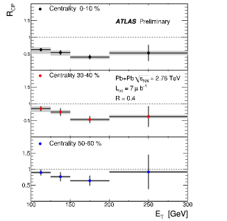
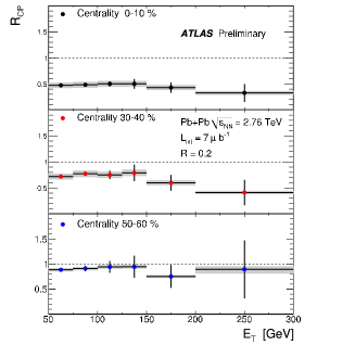
Fig. 1-a	Fig. 1-b

Figure 1: Nuclear modification factor(NMF) for jet production. The figures are taken from Ref.ATLAS

Let us first discuss the factorization theorem and why this theorem at first sight leads to the NMF equal to 1.

Indeed, the factorization theorem states that the inclusive cross section for gluon production with rapidity $Y^{\prime}$ and transverse momentum $p_{T}$ can be written asFT1 ; FT2 ; FT3 ; FT4

$$\frac{d^{2}\sigma\left(Y^{\prime},p_{T}\right)}{dY^{\prime}d^{2}p_{T}}\,=\,\sigma_{hard}\bigotimes x_{1}G_{Pr}\left(x_{1},\mu_{F}\right)x_{2}G_{Tr}\left(x_{2},\mu_{F}\right)\,\,\,\,\,\mbox{where}\,\,\,\,x_{1}\,=\frac{p_{T}}{\sqrt{s}}e^{Y^{\prime}}\,\,\mbox{and}\,\,x_{2}\,=\frac{p_{T}}{\sqrt{s}}e^{-Y^{\prime}}$$ (1)

where $\sqrt{s}=W$ is the energy of colliding particles and $\bigotimes$ denotes all necessary integrations while $\mu_{T}$ is the factorization scale which should be chosen of the order of $p_{T}$ of produced gluon. Eq. (1) has a simple meaning, namely that the production of a high $p_{T}$ gluon is proportional to the cross section of the interaction of two partons, with fractions of energy $x_{1}$ and $x_{2}$, multiplied by the probability to find them in the projectile ($G_{Pr}$) and target ($G_{Tr}$). All interactions in the final state as well as corrections to the initial state (for, example, due to shadowing) lead to small small contributions of the order of $1/p^{2}_{T}$.

At short distances (large $p_{T}$) the gluon structure function for a nucleus is equal to

$$xG_{A}\left(x,\mu_{T}\right)\,=\,AxG_{P}\left(x,\mu_{T}\right)$$ (2)

where $G_{P}$ is the nucleon gluon structure function. Therefore,

$$\frac{d^{2}\sigma\left(A_{1}+A_{2}|Y^{\prime},p_{T}\right)}{dY^{\prime}d^{2}p_{T}}\,\,=\,\,\,A_{1}A_{2}\frac{d^{2}\sigma\left(P+P|Y^{\prime},p_{T}\right)}{dY^{\prime}d^{2}p_{T}}$$ (3)

where $d^{2}\sigma\left(P+P|Y^{\prime},p_{T}\right)\Big{/}dY^{\prime}d^{2}p_{T}$ is the cross section of inclusive production in proton-proton collisions.

In other words the nuclear modification factor (NMF) $R_{AA}$, which is defined as

$$R_{AA}\,\,\,=\,\,\,\frac{\frac{d^{2}\sigma\left(A_{1}+A_{2}|Y^{\prime},p_{T}\right)}{dY^{\prime}d^{2}p_{T}}}{N_{coll}\,\frac{d^{2}\sigma\left(P+P|Y^{\prime},p_{T}\right)}{dY^{\prime}d^{2}p_{T}}}\,\,\,=\,\,\,1$$ (4)

where $N_{coll}$ is the number of collision that is equal to $A_{1}\,A_{2}$, in the case of large $p_{T}$.

The main result of this letter is that Eq. (2) should to be replaced by

$$xG_{A}\left(x,\mu^{2}_{F}/Q^{2}_{s}\left(A;x_{0}\right)\right)\,=\,AxG_{P}\left(x,\mu^{2}_{F}/Q^{2}_{s}\left(A;x_{0}\right)\right)\,=AxG_{P}\left(x,\mu^{2}_{F}/\Big{(}A^{1/3}Q^{2}_{s}\left(P;x_{0}\right)\Big{)}\right)\,\,\,\mbox{for}\,\,\mu_{F}\,\approx\,p_{T}\gg\,\,Q_{s}\left(A;x\right)$$ (5)

where $Q_{s}\left(A;x\right)$ ($Q_{s}\left(P;x\right)$) are the saturation momenta at $Y=\ln(1/x)$ for the nucleus and the proton, respectively. $Y_{0}=\ln(1/x_{0})$ is the rapidity at which the evolution starts. In other word, we state that the linear DGLAP or BFKL evolution should be started at different initial condition at low energy ($Y=Y_{0}$).

It follows from Eq. (5), that Eq. (4) reads as

$$R_{AA}\,\,\,=\,\,\,\frac{\frac{d^{2}\sigma\left(A_{1}+A_{2}|Y^{\prime},p_{T}\right)}{dY^{\prime}d^{2}p_{T}}}{N_{coll}\,\frac{d^{2}\sigma\left(P+P|Y^{\prime},p_{T}\right)}{dY^{\prime}d^{2}p_{T}}}\,\,\,=\,\,\,\frac{x_{1}G_{P}\left(x_{1},\mu^{2}_{F}/Q^{2}_{s}\left(A;x_{10}\right)\right)\,x_{2}G_{P}\left(x_{2},\mu^{2}_{F}/Q^{2}_{s}\left(A;x_{20}\right)\right)}{x_{1}G_{P}\left(x_{1},\mu^{2}_{F}/Q^{2}_{s}\left(P;x_{10}\right)\right)x_{1}G_{P}\left(x_{2},\mu^{2}_{F}/Q^{2}_{s}\left(P;x_{20}\right)\right)}$$ (6)

For the sake of numerical estimates we will derive the QCD factorization formula from the $k_{T}$-factorization, in order to specify the factorization scale $\mu_{F}$ and all numerical coefficients in Eq. (6). Using $k_{T}$ factorization KTF1 ; KTF2 ; KTF3 ; KTF4 , the inclusive cross section has the form

$$\frac{d\sigma}{dy\,d^{2}p_{T}}\,\,=\,\,\frac{2\pi\bar{\alpha}_{s}}{p^{2}_{T}}\int d^{2}k_{T}\,\,\phi^{A_{1}}_{G}\left(x_{1};\vec{k}_{T}\right)\,\phi^{A_{2}}_{G}\left(x_{2};\vec{p}_{T}-\vec{k}_{T}\right)$$ (7)

where $\phi^{A_{i}}_{G}$ is the probability to find a gluon in the nucleus ($A_{i}$), that carries the fraction of energy $x_{i}$ with $k_{T}$ transverse momentum, and $\bar{\alpha}_{s}\,=\,\alpha_{s}N_{c}/\pi$, where $N_{c}$ is equal to the number of colours in the $SU_{N_{c}}$ colour group. At large values of $p_{T}$ we can re-write Eq. (7) in the form

$$\frac{d\sigma}{dy\,d^{2}p_{T}}\,\, = \,\,\frac{2\pi\bar{\alpha}_{s}}{p^{2}_{T}}\Big{\{}\int^{p_{T}}d^{2}k_{T}\phi^{A_{1}}_{G}\left(x_{1};\vec{k}_{T}\right)\phi^{A_{2}}_{G}\left(x_{2};\vec{p}_{T}\right)\,+\,\phi^{A_{1}}_{G}\left(x_{1};\vec{p}_{T}\right)\int^{p_{T}}d^{2}k_{T}\phi^{A_{2}}_{G}\left(x_{2};\vec{k}_{T}\right)\Big{\}}\,\,$$ (8)

$$= \,\,\frac{2\pi\bar{\alpha}_{s}}{p^{2}_{T}}\,\frac{d}{dp^{2}_{T}}\Big{(}x_{1}G_{A_{1}}\left(x_{1},p^{2}_{T}\right)x_{2}G_{A_{2}}\left(x_{2},p^{2}_{T}\right)\Big{)}$$

For the purpose of deriving Eq. (8), we used the relation between the un-integrated gluon density $\phi$ and the gluon structure function (see for example Ref.GLR ):

$$xG\left(x,Q^{2}\right)\,\,=\,\,\int^{Q^{2}}_{0}\,\phi\left(k^{2}_{T}\right)dk^{2}_{T}$$ (9)

Using Eq. (8) one can see that Eq. (6) can be rewritten as

$$R_{AA}\,\,\,=\,\,\frac{\frac{d}{dp^{2}_{T}}\Big{(}x_{1}G_{P}\left(x_{1},p^{2}_{T}/Q^{2}_{s}\left(A;x_{10}\right)\right)\,x_{2}G_{P}\left(x_{2},p^{2}_{T}/Q^{2}_{s}\left(A;x_{20}\right)\right)\Big{)}}{\frac{d}{dp^{2}_{T}}\Big{(}x_{1}G_{P}\left(x_{1},p^{2}_{T}/Q^{2}_{s}\left(P;x_{10}\right)\right)\,x_{2}G_{P}\left(x_{2},p^{2}_{T}/Q^{2}_{s}\left(P;x_{20}\right)\right)\Big{)}}$$ (10)

II Relation $xG_{A}\left(x,p^{2}_{T}/Q^{2}_{s}\left(A;x_{0}\right)\right)\,=\,AxG_{P}\left(x,p^{2}_{T}/\Big{(}A^{1/3}Q^{2}_{s}\left(P;x_{0}\right)\Big{)}\right)$

The proof of Eq. (5) is based on two observations. First, the equations in the region of low $x$ can be written as an evolution in rapidity, both in the approach of DGLAP DGLAP and in the BFKL BFKL approach. They both have the following general form

$$\frac{\partial xG\left(Y;p^{2}_{T}\right)}{\partial Y}\,\,=\,\,\int d^{2}k_{T}\,K\left(p_{T},k_{T}\right)\,xG\left(Y,k^{2}_{T}\right)$$ (11)

where $Y=\ln(1/x)$.

Second, since for large $p_{t}$ we can restrict ourselves to the linear evolution: DGLAP or BFKL, one can see that the solution of Eq. (11) can be written as

$$xG\Big{(}Y,\xi\equiv\,\ln\left(p^{2}_{T}/\Lambda^{2}_{QCD}\right)\Big{)}\,\,=\,\,\int d\xi^{\prime}\,G\left(Y-Y_{0},\xi-\xi^{\prime}\right)\,xG_{in}\left(Y=Y_{0},\xi^{\prime}\right)$$ (12)

where $G\left(Y-Y_{0},\xi-\xi^{\prime}\right)$ is the Green function of Eq. (11): the solution to Eq. (11) with the initial condition $G\left(Y=Y_{0},\xi-\xi^{\prime}\right)\,=\,\delta\left(\xi-\xi^{\prime}\right)$. $xG_{in}\left(Y=Y_{0},\xi^{\prime}\right)$ is the initial condition for the gluon structure function.

For linear evolution the solution to the equation reveals the following property of the propagator GLR ; MUSH ; KLM :

$$xG\Big{(}Y,\xi\equiv\,\ln\left(p^{2}_{T}/\Lambda^{2}_{QCD}\right)\Big{)}\,\,=\,\,\int\,d\xi^{\prime}\,\,G\left(Y-Y^{\prime},\xi-\xi^{\prime}\right)\,xG\left(Y^{\prime},\xi^{\prime}\right)$$ (13)

for any value of $Y^{\prime}$. We can prove Eq. (13) by solving Eq. (11) using the double Mellin transform

$$xG\left(Y,\xi\right)\,\,\,=\,\,\int^{\epsilon+i\infty}_{\epsilon-i\infty}\frac{d\omega}{2\pi i}\,\int^{\epsilon+i\infty}_{\epsilon-i\infty}\frac{d\gamma}{2\pi i}\,e^{\omega Y+\gamma\xi}\,g\left(\omega,\gamma\right)$$ (14)

Plugging Eq. (14) into Eq. (11) we obtain the solution

$$\omega\,\,=\,\,\omega\left(\gamma\right)$$ (15)

where $\omega\left(\gamma\right)$ is the Mellin image of the kernel in Eq. (11). It can be verified that the Green function has the form

$$G\left(Y-Y^{\prime},\xi\right)\,\,\,=\,\,\,\int^{\epsilon+i\infty}_{\epsilon-i\infty}\frac{d\gamma}{2\pi i}\,e^{\omega\left(\gamma\right)\left(Y-Y^{\prime}\right)\,+\,\gamma\left(\xi-\xi^{\prime}\right)}\,$$ (16)

while the solution of Eq. (12) can be written in two equivalent forms

$$xG\left(Y,\xi\right)\,\,\,=\,\,\,\int^{\epsilon+i\infty}_{\epsilon-i\infty}\frac{d\gamma}{2\pi i}\,e^{\omega\left(\gamma\right)Y+\gamma\xi}\,g_{in}\left(\gamma\right)\,\,=\,\,\int^{\epsilon+i\infty}_{\epsilon-i\infty}\frac{d\omega}{2\pi i}\,e^{\omega Y+\gamma\left(\gamma\right)\,\xi}\,g_{in}\left(\omega\right)$$ (17)

where $g_{in}$ is the Mellin image of $xG_{in}\left(Y=Y_{0},\xi^{\prime}\right)$ in Eq. (12) and $\gamma\left(\omega\right)$ is the anomalous dimension which can be obtained as solution of Eq. (15).

Using Eq. (16) and Eq. (17) for the r.h.s. of Eq. (13), and integrating over $\xi^{\prime}$ we obtain the l.h.s. of this equation.

Our standard approach to low $x$ evolution consists of two steps. First, we assume that there exists a small $x=x_{0}$ ($Y=Y_{0}=\ln(1/x_{0})$) which is large ($Y_{0}\gg 1$), but at the same time small enough such that $\bar{\alpha}_{s}Y_{0}\ll 1$ . For this type of $Y_{0}$ we have the theoretical formula (the McLerram-Venugopalan formula MV ) for the scattering amplitude of the dipole,which looks as follows in the most simplified form

$$N\left(r,b;Y_{0}\right)\,\,=\,\,1\,\,-\,\,\exp\left(-r^{2}Q^{2}_{s}\left(Y_{0},b\right)/4\right)$$ (18)

where $N$ is the imaginary part of the scattering amplitude; $Q_{s}$ is the saturation scale at $Y=Y_{0}$ , $r$ is the dipole size and $b$ is the impact parameter. The main features of Eq. (18) are that the amplitude of Eq. (18) has the geometric scaling behaviour GS at low energy ($Y=Y_{0}$), since it is a function of only one argument $N\left(r,b;Y_{0}\right)\,=\,N\left(\tau\equiv r^{2}Q_{s}\left(Y_{0},b\right)\right)$.

The second step is to use the evolution in the region $Y>Y_{0}$. In our case, when the typical size of the dipole is small ($r\approx 1/p_{T}$), we can use the linear BFKL or DGLAP equations. It should be stressed that we use the rigorous theoretical formula of Eq. (18), which shows the geometric scale behaviour only for the initial condition, for the linear evolution.

We will show below that for the initial condition $x_{0}G\left(Y_{0},k_{T}\right)\,=\,S\,Q^{2}_{s}(Y_{0})g\left(\tau=k^{2}_{T}/Q^{2}_{s}\left(Y\right)\right)$. Using Eq. (13) with $Y^{\prime}=Y_{0}$ we have

$$xG\Big{(}Y,\xi\equiv\,\ln\left(p^{2}_{T}/\Lambda^{2}_{QCD}\right)\Big{)}\,\, = \,\,\int\,d\xi^{\prime}\,\,G\left(Y-Y_{0},\xi-\xi^{\prime}\right)\,x_{0}G\left(Y_{0},\xi^{\prime}\right)\,\,$$ (19)

$$= \,\,S\,Q^{2}_{s}\left(Y_{0}\right)\int\frac{dk^{2}_{T}}{k^{2}_{T}}G\left(Y-Y_{0},p^{2}_{T}/k^{2}_{T}\right)\,g\left(k^{2}_{T}/Q^{2}_{s}\left(Y_{0}\right)\right)$$

$$= \,\,\,S\,Q^{2}_{s}(Y_{0})\,\int^{\epsilon+i\infty}_{\epsilon-i\infty}\frac{d\gamma}{2\pi i}\,e^{\omega\left(\gamma\right)\left(Y-Y_{0}\right)}\,\left(\frac{p_{T}^{2}}{k^{2}_{T}}\right)^{\gamma}\,g\left(\frac{k^{2}_{T}}{Q^{2}_{s}\left(Y_{0}\right)}\right)$$

$$= \,\,S\,Q^{2}_{s}(Y_{0})\,\int^{\epsilon+i\infty}_{\epsilon-i\infty}\frac{d\gamma}{2\pi i}\,e^{\omega\left(\gamma\right)\left(Y-Y_{0}\right)}\,\left(\frac{p_{t}^{2}}{Q^{2}_{s}\left(Y_{0}\right)}\right)^{\gamma}\int\frac{d\tau}{\tau}\tau^{-\gamma}\,g\left(\tau\right)$$

$$= \,\,\,S\,Q^{2}_{s}(Y_{0})\,\int^{\epsilon+i\infty}_{\epsilon-i\infty}\frac{d\gamma}{2\pi i}\,e^{\omega\left(\gamma\right)\left(Y-Y_{0}\right)}\,\left(\frac{p_{t}^{2}}{Q^{2}_{s}\left(Y_{0}\right)}\right)^{\gamma}f\left(\gamma\right)$$

where $\tau=k^{2}_{T}/Q^{2}_{s}$ and $S$ is the area of the target. In Eq. (19) we used Eq. (16). The function $f(\gamma)$ does not depend on the character of the target, and it is the same for the nucleus and for the nucleon if we consider Eq. (18) for both. Since $Q_{s}\left(A;Y_{0}\right)\,\,=\,\,A^{1/3}\,Q_{s}\left(P;Y_{0}\right)$ and $S_{A}=A^{2/3}$ , one can see that Eq. (5) follows from Eq. (19).

Now let us show that $x_{0}G\left(Y_{0},k_{T}\right)\,=\,S\,Q^{2}_{s}(Y_{0})g\left(\tau\right)$. The relation between $\phi^{A}_{G}\left(x;\vec{k}_{T}\right)$ and the dipole scattering amplitude $N\left(x,r;b\right)$ has the form KTINC

$$\phi^{A}_{G}\left(x_{0};\vec{k}_{T}\right)\,\,=\,\,\frac{1}{\bar{\alpha}_{s}\,4\pi}\,\int d^{2}b\,d^{2}re^{i\vec{k}_{T}\cdot\vec{r}}\,\,\nabla^{2}_{\perp}\,N^{A}_{G}\left(Y_{0};r;b\right)$$ (20)

where

$$N^{A}_{G}\left(Y_{0};r,b\right)\,\,=\,\,2\,N\left(Y_{0};r,b\right)\,\,\,-\,\,\,N^{2}\left(Y_{0};r,b\right)\xrightarrow{{Eq.~{}(\ref{MVF})}}\,1\,\,-\,\,\exp\left(-r^{2}Q^{2}_{s}\left(Y_{0};b\right)/2\right)$$ (21)

Plugging Eq. (21) into Eq. (20) and using the simplest model for the $b$ dependence, viz. $Q_{s}^{2}\left(Y_{0};b\right)\,\,=\,\,Q_{s}\left(Y_{o}\right)\Theta\left(R_{A}-b\right)$ we obtain

$$\phi^{A}_{G}\left(x_{0};\vec{k}_{T}\right)\,\,=\phi^{A}_{G}\left(\tau=k^{2}_{T}/Q^{2}_{s}\left(Y_{0}\right)\right)\,\,=\,\,\,2\pi\,S\,\tau\,\exp\left(-2\,\tau\right)$$ (22)

Using Eq. (9) we calculate the gluon structure function at $Y=Y_{0}$. It is equal to

$$x_{0}G\left(x_{0},p^{2}_{T}\right)\,\,=\,\,\frac{\pi}{2}S\,Q^{2}\left(Y_{)}\right)\,\Big{(}1\,-\,\left(1+2\,\tau\right)\,\exp\left(-2\tau\right)\Big{)}\,\,=\,\,S\,Q^{2}_{s}\left(Y_{0}\right)\,g\left(\tau\right)$$ (23)

Therefore, we arrive at the result $x_{0}G\left(Y_{0},k_{T}\right)\,=\,S\,Q^{2}_{s}(Y_{0})g\left(\tau\right)$ with the particular function $g\left(\tau\right)$. The corresponding function $f\left(\tau\right)$ (see Eq. (19)) turns out to be equal to $f\left(\tau\right)\,=\,2^{\gamma}\Gamma\left(2-\gamma\right)/\gamma$.

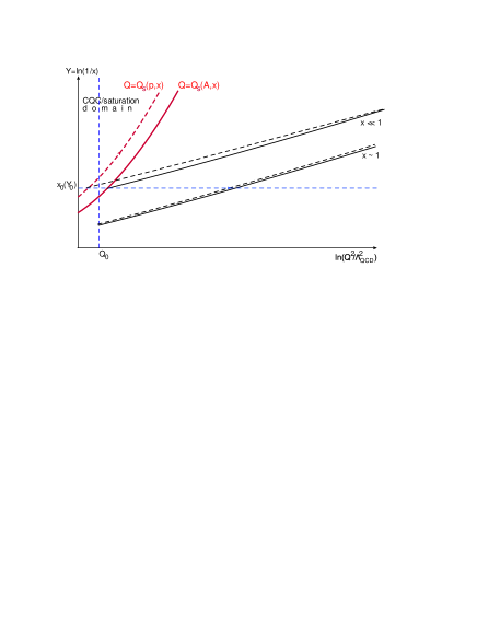
Figure 2: The semi-classical trajectories for the nucleus (solid lines) and nucleon (dashed lines) gluon structure function in the region of large and small $x$. In the Color Glass Condensate (CGC)/saturation domain the structure function has a geometric scaling behaviour.

Eq. (19) is the main result of the paper. It should be stressed that solution which we found, does not lead to the geometric scaling behaviour since it depends on both variable: $x$ and $p_{T}$. However, Eq. (19) shows that $p_{T}$ in the DGLAP evolution scales with different momentum that depends on the target. In this sense this equation shows the $p_{T}$ scaling behaviour. The fact that in DGLAP evolution $p_{T}$ is scaled by the typical momentum in the initial condition is well known and follows directly from the conformal symmetry of the DGLAP equation at fixed QCD coupling. Two ideas are new in the proof of Eq. (19): the evolution at low $x$ has to start with rather low initial $x_{0}$ and the initial condition at this $x=x_{0}$ has to show the geometric scaling behaviour. Both of these results follows from the Color Glass Condensate/saturation approach and are rigorous results for QCD.

To illustrate the situation we consider the semi-classical approach to the solution of the DGLAP equationsSCL . In this approach we take the integral over $\gamma$ in Eq. (19) using the steepest decent method and the solution is characterized by the trajectory: the line in $(\ln(1/x),\ln\left(Q^{2}/\Lambda^{2}_{QCD}\right)$ plane. The trajectory shows what values of $x_{0}$ and $Q_{0}$ in the initial condition are essential to find the solution in the point $\left(\ln(1/x),\ln\left(Q^{2}/\Lambda^{2}_{QCD}\right)\right)$. Fig. 2 shows the trajectories for gluon structure function in the region of low $x$ and in the region of $x\sim 1$. These trajectories are denoted by solid and dashed lines for nucleus and nucleon targets, respectively. On can see that for $x\sim 1$ both trajectory for nucleus and for proton targets started at the value of $Q=Q_{0}$ which corresponds to the same scaling of $p_{T}$ for interaction with nucleus and nucleon. However, for the region of low $x$ the situation changes crucially and the evolution starts from the value of $Q_{0}$ that should be determined by the initial condition given by the Color GlassCondensate/saturation approach. Fig. 2 illustrates the main result of the CGC/saturation approach: we cannot use the initial condition at fixed arbitrary $Q=Q_{0}$ since its contradicts the unitarity constraints.

III Estimates for NMF

At first sight the value for $R_{AA}$ could be calculated in a direct way, just by using Eq. (6) and various different fits to the available DIS data, using the DGLAP evolution equations. By plugging in Eq. (6) the gluon structure functions that are available on the market (see Ref.DISSTR ) and using $Q^{2}_{s}\left(A;Y_{0}\right)=A^{1/3}Q^{2}_{s}\left(P;Y_{0}\right)$ , then we obtain $R_{AA}$ for the gluon jet production at the LHC, in the central rapidity region for the lead-lead collisions. This estimates are shown by the black line in Fig. 3. In Fig. 3 are plotted the NMF using the MRSTW parameterization MRSTW but we check that the other parameterizations give approximately the same value for $R_{AA}$.

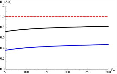
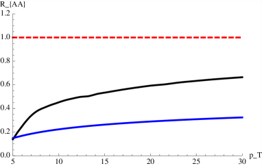
Fig. 3-a		Fig. 3-b

Figure 3: Nuclear modification factor (NMF) for jet production. The black line shows $R_{AA}$ from Eq. (6) for MRSTW parameterizations of the gluon structure functions (see Ref.MRSTW . $R_{AA}$ from Eq. (25) is plotted by the blue line. $\bar{\alpha}_{s}$ is taken to be $\bar{\alpha}_{s}=0.2$ and $x_{1}=x_{2}=10^{-3}$

However, this type of approach suffers from two major defects. First, in all parameterizations the running QCG coupling is used. The transverse momenta $p_{T}$ enters to the expression for the running QCD coupling as $\ln\left(p^{2}_{T}/\Lambda_{QCD}\right)$ and, therefore, they are not rescaled with the saturation momenta. Second, the gluon structure functions, that we used, where extracted from the experimental data using the DGLAP evolution in transverse momenta, but not in $Y$ .

We believe that we can obtain more reliable estimates by using Eq. (19), Eq. (17) and Eq. (23). It is known that the leading order DGLAP anomalous dimension can be approximated with an accuracy of 5$\%$ by the following expression EKL

$$\gamma\,\,=\,\ \bar{\alpha}_{s}\Big{(}\frac{1}{\omega}\,-\,1\Big{)}\,\,\,\,\,\mbox{or}\,\,\,\,\,\,\omega\left(\gamma\right)\,\,=\,\,\frac{\alpha_{s}}{\gamma\,+\,\bar{\alpha}_{s}}$$ (24)

Substituting $\omega(\gamma)$ from Eq. (24) and taking the integral using the steepest decent method, we obtain the following answer:

$$xG\left(Y,\tau=\right)\,\,=\,\,f\left(\gamma_{SP}\right)\,\exp\Big{(}2\,\sqrt{\bar{\alpha}_{s}\,Y\,\ln\left(\tau\right)}\,\,-\,\,\bar{\alpha}_{s}\,\ln\left(\tau\right)\Big{)}\,\,\,\,\mbox{with}\,\,\,\,\,\gamma_{SP}\,\,=\,\,\sqrt{\frac{\bar{\alpha}_{s}Y}{\ln\left(\tau\right)}}\,\,-\,\,\bar{\alpha}_{s}$$ (25)

where $\tau=p^{2}_{T}/Q^{2}_{s}\left(Y_{0}\right)$ and $Y=\ln(1/x)$.

The blue curve in Fig. 3 describes $R_{AA}$ from Eq. (10) with the gluon structure function given by Eq. (25). This estimate leads to smaller values of $R_{AA}=0.4\div 0.5$ (see Fig. 3).

Using the KLN approach KLN , we can estimate $R_{CP}$ which is defined as

$$R_{CP}\,\, = \,\,\frac{1}{N^{centr}_{coll}}\frac{dN^{centr}}{dYd^{2}p_{T}}{\Big{/}}\frac{1}{N^{periph}_{coll}}\frac{dN^{periph}}{dYd^{2}p_{T}}\,\,$$

$$= \,\,\frac{\frac{d}{dp^{2}_{T}}\Big{(}x_{1}G_{P}\left(x_{1},p^{2}_{T}/Q^{2}_{s}\left(centr;x_{10}\right)\right)\,x_{2}G_{P}\left(x_{2},p^{2}_{T}/Q^{2}_{s}\left(centr;x_{20}\right)\right)\Big{)}}{\frac{d}{dp^{2}_{T}}\Big{(}x_{1}G_{P}\left(x_{1},p^{2}_{T}/Q^{2}_{s}\left(periph;x_{10}\right)\right)\,x_{2}G_{P}\left(x_{2},p^{2}_{T}/Q^{2}_{s}\left(periph;x_{20}\right)\right)\Big{)}}$$

where $N^{centr}_{coll}$($Q\left(centr;Y_{0}\right)$) and $N^{periph}_{coll}$($Q\left(periph;Y_{0}\right)$) are the number of collisions ( saturation momentum) in the events with fixed centrality and for peripheral collision, respectively. Based on the KLN approach we know the saturation momentum for the events with fixed centrality, and using Eq. (III) we calculate the $R_{CP}$ (see Fig. 4).

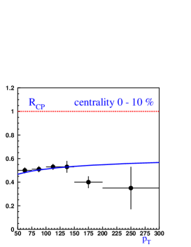
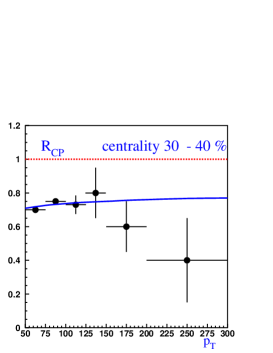
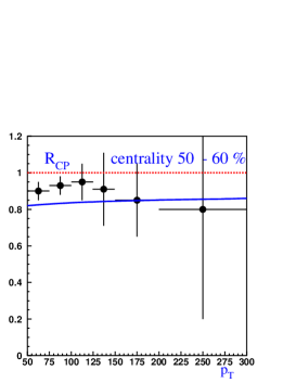
Figure 4: Nuclear modification factor (NMF) for jet production. The data is taken from Ref.ATLAS . The curves are calculated from Eq. (III) while the value of the saturation momenta for each centrality events are estimated in the KLN-procedure KLN , with the number of participants taken from Ref.ATLAS . The peripheral collisions are the events with centrality $80\div 100\%$. The values of $x_{1}$ and $x_{2}$ are chosen to be $x_{1}=x_{2}=10^{-3}$.

IV Conclusions

The main result of the paper is that the two questions which have been formulated in the introduction, namely, could we obtain the NMF less that unity for production of gluon at very high energy (small $x$) and with large value of transverse momentum, without violation of the factorization theorem; and can be the value of NMF of the order of the value measured by ATLAS, have the affirmative answers.

Eq. (5) shows that the NMF for the gluon jet production turns out to be less than 1. This equation is proven using two main ingredients from the Colour Glass Condensate (CGC)/saturation approach: the typical $x_{0}$ in the initial condition for the evolution in the region of low $x$ even at high values of $p_{T}$ is rather low and we need to use the Color Glass Condensate approach to describe them; and the initial condition at fixed $Y=Y_{0}$ depends on one variable $\tau=p^{2}_{T}/Q^{2}_{s}(Y_{0})$, and this initial condition has the same form for the scattering with nuclei and protons. The last assumption is essential for the estimates of $R_{AA}$, but not for $R_{CP}$. For $R_{CP}$ we can use a weaker assumption, namely, that the McLerran-Venugopalan formula can be used for the description of the peripheral collisions.

As have been claimed in the introduction we do not pretend that we can describe the data since we consider the theoretical example of very small and fixed $x$ and large values of $p_{T}$ . The kinematical region were the experimental data are taken, perhaps, is quite different. Our estimates show that the scale of the effect is of the oder of the experimental one. Therefore, the fact that we do not reach a good agreement with the experimental data does not discourage us. It should be mentioned that the simple formula that we use (see Eq. (25)) relies on the saddle point approximation, and on the particularly simple form of Eq. (18) for the McLerran-Venugopalan formula.

For serious comparison with the experimental data we have to develop an approach similar to one in Ref.ALMAR . We believe that we find the explanation, why NMF calculated in this paper as well is in many others based on CGC approach , lead to the value of the NMF less than unity.

The conclusion from the paper can be formulated in one sentence: the NMF can be smaller that unity for jet production at low and fixed $x$ and at large transverse momentum $p_{T}$ without any violation of the factorization theorem and the initial state effects are able to explain the NMF of the order of the one measured by ATLAS. In other word, initial state effects are able to describe the jet quenching for the gluon jet production.

This mechanism leads to stronger suppression at smaller value of $p_{T}$ (see Fig. 3-b) and it should be taken into account in the explanation of the NMF for produced hadrons.

V Acknowledgements

We thank Boris Kopeliovich for fruitful discussions on the subject, that convinced me that the origin of the NMF is deeper than the interaction of the jet in the final state. This research was supported by the Fondecyt (Chile) grant 1100648.

References

(1)
ATLAS collaboration: “Centrality dependence of Jet Yields and Jet Fragmentation in Lead-Lead
Collisions at with the ATLAS detector at the LHC”, ATLAS-CONF-2011-075.
(2)
J. C. Collins, D. E. Soper and G. F. Sterman,
Adv. Ser. Direct. High Energy Phys. 5 (1988) 1
[arXiv:hep-ph/0409313].
(3)
J. C. Collins, D. E. Soper and G. F. Sterman,
Nucl. Phys. B 308 (1988) 833.
(4)
G. T. Bodwin,
Phys. Rev. D 31 (1985) 2616
[Erratum-ibid. D 34 (1986) 3932]
[Phys. Rev. D 34 (1986) 3932].
(5)
J. C. Collins, D. E. Soper and G. F. Sterman,
Nucl. Phys. B 261 (1985) 104.
(6)
Z. Chen and A. H. Mueller,
Nucl. Phys. B 451 (1995) 579; Y. V. Kovchegov and K. Tuchin,
Phys. Rev. D 65 (2002) 074026
[hep-ph/0111362].
(7)
S. Catani, M. Ciafaloni and F. Hautmann,
Nucl. Phys. B 366 (1991) 135.
(8)
S. Catani, M. Ciafaloni and F. Hautmann,
Nucl. Phys. Proc. Suppl. 29A (1992) 182.
(9)
J. C. Collins and R. K. Ellis,
Nucl. Phys. B 360 (1991) 3.
(10)
E. M. Levin, M. G. Ryskin, Yu. M. Shabelski and A. G. Shuvaev,
Sov. J. Nucl. Phys. 53 (1991) 657
[Yad. Fiz. 53 (1991) 1059].
(11)
V. N. Gribov and L. N. Lipatov, Sov. J. Nucl. Phys 15 (1972)
438;
G. Altarelli and G. Parisi, Nucl. Phys. B 126 (1977) 298;
Yu. l. Dokshitser, Sov. Phys. JETP 46 (1977) 641.
(12)
E. A. Kuraev, L. N. Lipatov, and F. S. Fadin, Sov. Phys. JETP
45 (1977) 199 ;
Ya. Ya. Balitsky and L. N. Lipatov,
Sov. J. Nucl. Phys. 28 (1978) 22 .
(13)
L. V. Gribov, E. M. Levin and M. G. Ryskin,
Phys. Rep. 100 (1983) 1.
(14)
A. H. Mueller, A. I. Shoshi,
Nucl. Phys. B692, 175-208 (2004).
[hep-ph/0402193].
(15)
D. Kharzeev, E. Levin, L. McLerran,
Phys. Lett. B561 (2003) 93-101.
[hep-ph/0210332
(16)
L. McLerran and R. Venugopalan,
Phys. Rev. D49 (1994) 2233, D49 (1994) 3352; D50 (1994) 2225;
D59 (1999) 094002.
(17)
J. Bartels and E. Levin,
Nucl. Phys. B 387 (1992) 617;
A. M. Stasto, K. J. Golec-Biernat and J. Kwiecinski,
Phys. Rev. Lett. 86 (2001) 596
[arXiv:hep-ph/0007192]; E. Iancu, K. Itakura and L. McLerran,
Nucl. Phys. A 708 (2002) 327
[arXiv:hep-ph/0203137].
(18)
Y. V. Kovchegov and K. Tuchin,
Phys. Rev. D 65 (2002) 074026
[arXiv:hep-ph/0111362].
(19)
J. C.Collins and J. Kwiecinski
Nucl. Phys. B 335 (1990) 89;
J. Bartels, G. A. Schuler and J. Blumlein,
Z. Phys. C 50 (1991) 91; ,
E. Laenen and E. Levin,
Ann. Rev. Nucl. Part. Sci. 44 (1994) 199;
S. Bondarenko, M. Kozlov and E. Levin,
Nucl. Phys. A727 (2003) 139.
(20)
A. D. Martin, W. J. Stirling, R. S. Thorne and G. Watt,
Eur. Phys. J. C 70 (2010) 51
[arXiv:1007.2624 [hep-ph]] and references therein.
(21)
See Durham database:
http://hepdata.cedar.ac.uk/pdfs
(22)
D. Kharzeev, E. Levin and M. Nardi,
Nucl. Phys. A 730 (2004) 448
[Erratum-ibid. A 743 (2004) 329]
[arXiv:hep-ph/0212316]; Phys. Rev. C 71 (2005) 054903
[arXiv:hep-ph/0111315]; D. Kharzeev and E. Levin,
Phys. Lett. B 523 (2001) 79
[arXiv:nucl-th/0108006]; D. Kharzeev and M. Nardi,
Phys. Lett. B 507 (2001) 121
[arXiv:nucl-th/0012025];
D. Kharzeev, E. Levin and M. Nardi,
Nucl. Phys. A 747 (2005) 609
[arXiv:hep-ph/0408050].;
A. Dumitru, D. E. Kharzeev, E. M. Levin and Y. Nara,
“Gluon saturation in collisions at the LHC: KLN model predictions for hadron multiplicities,”
arXiv:1111.3031 [hep-ph].
(23)
R. K. Ellis, Z. Kunszt and E. M. Levin,
Nucl. Phys. B 420, 517 (1994)
[Erratum-ibid. B 433, 498 (1995)].
(24)
J. C. Albacete and C. Marquet, Phys. Lett. B 687 (2010) 174,
[arXiv:1001.1378 (hep-ph)] and references there in.