A simple closure approximation for slow dynamics of a multiscale system: nonlinear and multiplicative coupling

Abstract

Multiscale dynamics are ubiquitous in applications of modern science. Because of time scale separation between relatively small set of slowly evolving variables and (typically) much larger set of rapidly changing variables, direct numerical simulations of such systems often require relatively small time discretization step to resolve fast dynamics, which, in turn, increases computational expense. As a result, it became a popular approach in applications to develop a closed approximate model for slow variables alone, which both effectively reduces the dimension of the phase space of dynamics, as well as allows for a longer time discretization step. In this work we develop a new method for approximate reduced model, based on the linear fluctuation-dissipation theorem applied to statistical states of the fast variables. The method is suitable for situations with quadratically nonlinear and multiplicative coupling. We show that, with complex quadratically nonlinear and multiplicative coupling in both slow and fast variables, this method produces comparable statistics to what is exhibited by an original multiscale model. In contrast, it is observed that the results from the simplified closed model with a constant coupling term parameterization are consistently less precise.

1 Introduction

Multiscale dynamics are ubiquitous in applications of modern science, with geophysical science and climate change prediction being well-known examples [14, 15, 10, 23]. Direct numerical simulations of multiscale systems are difficult, both because a relatively short time discretization step is required to resolve fast dynamics, and due to a large number of dynamical variables. Moreover, in some applications such as climate change prediction one is interested in long-term statistics of slow dynamics, which further increases computational expense.

A popular approach for simulating multiscale dynamics in practice with limited computational resources is to create an approximate reduced model for slow variables alone, which allows to increase the length of the time discretization step and reduced the dimension of the phase space of the system, which is accomplished via an approximate closure of the coupling terms between slow and fast variables of the system. Many closure methods were designed for multiscale dynamical systems [11, 13, 19, 22, 20, 21], based on the averaging formalism for the fast variables [24, 29, 30]. Some methods approximate the coupling terms with appropriate stochastic processes [19, 22, 20, 21, 31] or conditional Markov chains [11], while others [13] parameterize slow-fast interactions by direct tabulation and curve fitting.

In a recent work [4] the author developed a simple approach of computing the reduced model for slow variables alone via a single computation of relevant statistics for the fast dynamics with a fixed reference state of the slow variables, using the linear fluctuation-dissipation theorem (FDT) [1, 2, 3, 5, 7, 6, 8, 9, 18, 25]. It was shown that, for the appropriately rescaled two-scale Lorenz 96 model [5] with linear coupling between slow and fast variables, the method reproduced statistics of the slow variables of the complete two-scale Lorenz model with good precision. However, nonlinear coupling was not addressed in [4].

This work is a natural extension of the method in [4] onto quadratically nonlinear and multiplicative types of coupling in both slow and fast variables. It is also based on the linear FDT, which is used to compute the response of linear, nonlinear and multiplicative terms of the fast variables coupling to changes in the slow variables. We show numerical experiments for this method with the two-scale Lorenz model and general forms of coupling which include multiplicative and quadratically nonlinear terms.

The manuscript is organized as follows. In Section 2 we formulate the theory for the new method. In Section 3 we present the two-scale Lorenz model [13, 16, 17], rescaled in such a way that the mean states and variances of both the fast and slow variables are near zero and one, respectively [5, 4]. Section 4 shows the results of numerical simulations with both the two-scale Lorenz model and the reduced model for slow variables only, comparing different statistics of the time series. Section 5 summarizes the results of this work.

2 Derivation of the reduced model

We start with a general two-scale system of differential equations of the form

$$\frac{\mathrm{d}\boldsymbol{x}}{\mathrm{d}t}=\boldsymbol{F}(\boldsymbol{x},\boldsymbol{y}),\qquad\frac{\mathrm{d}\boldsymbol{y}}{\mathrm{d}t}=\boldsymbol{G}(\boldsymbol{x},\boldsymbol{y}),$$ (1)

where $\boldsymbol{x}=\boldsymbol{x}(t)\in\mathbb{R}^{N_{x}}$ are the slow variables, $\boldsymbol{y}=\boldsymbol{y}(t)\in\mathbb{R}^{N_{y}}$ are the fast variables, and $\boldsymbol{F}$ and $\boldsymbol{G}$ are $N_{x}$ and $N_{y}$ vector-valued functions of $\boldsymbol{x}$ and $\boldsymbol{y}$, respectively. We assume that the $\boldsymbol{y}$-variables are sufficiently fast for a valid approximation of the system in (1) by the averaged dynamics for $\boldsymbol{x}$, given by

$$\frac{\mathrm{d}\boldsymbol{x}}{\mathrm{d}t}=\langle\boldsymbol{F}\rangle(\boldsymbol{x}),\qquad\langle\boldsymbol{F}\rangle(\boldsymbol{x})=\int_{\mathbb{R}^{N_{y}}}\boldsymbol{F}(\boldsymbol{x},\boldsymbol{z})\,\mathrm{d}\mu_{\boldsymbol{x}}(\boldsymbol{z}),$$ (2)

for finite times (for a more detailed description of the averaging formalism, see [2, 5, 24, 29, 30]). Here, $\mu_{\boldsymbol{x}}$ denotes the invariant probability measure of the limiting fast dynamics, which are given by system

$$\frac{\mathrm{d}\boldsymbol{z}}{\mathrm{d}\tau}=\boldsymbol{G}(\boldsymbol{x},\boldsymbol{z}).$$ (3)

Above, $\boldsymbol{x}$ is a constant parameter, and the solution of (3) is given by the flow $\boldsymbol{z}(\tau)=\phi_{\boldsymbol{x}}^{\tau}\boldsymbol{z}_{0}$. We tacitly assume that all typical initial conditions $\boldsymbol{z}_{0}$ fall into the support of the same ergodic component of $\mu_{\boldsymbol{x}}$, and that $\langle\boldsymbol{F}\rangle(\boldsymbol{x})$ varies smoothly with respect to $\boldsymbol{x}$, as it often happens when $\mu_{\boldsymbol{x}}$ is an SRB measure [12, 27, 28, 26, 32]. Using the ergodicity assumption for $\mu_{\boldsymbol{x}}$, we can practically compute the measure average via the time average

$$\langle\boldsymbol{F}\rangle(\boldsymbol{x})=\lim_{r\to\infty}\frac{1}{r}\int_{0}^{r}\boldsymbol{F}(\boldsymbol{x},\boldsymbol{z}(\tau))\,\mathrm{d}\tau,$$ (4)

where $\boldsymbol{z}(\tau)$ is a long-term trajectory of (3).

Following [4], here we propose an approximation to $\langle\boldsymbol{F}\rangle(\boldsymbol{x})$, based on the linear FDT. In order to do this, certain assumptions have to be made regarding coupling, that is the dependence of $\boldsymbol{F}$ and $\boldsymbol{G}$ on the fast and slow variables, respectively. In [4] it was assumed that $\boldsymbol{F}$ depends linearly on the fast variables, and $\boldsymbol{G}$ depends linearly on the slow variables (linear coupling). Here we assume that $\boldsymbol{F}$ is quadratic in the fast variables in the vicinity of $\boldsymbol{\bar{z}}(\boldsymbol{x})$, which is the mean state of (3) with $\boldsymbol{x}$ set as a constant parameter:

$$\begin{split}\boldsymbol{F}(\boldsymbol{x},\boldsymbol{z})&=\boldsymbol{F}(\boldsymbol{x},\boldsymbol{\bar{z}}(\boldsymbol{x}))+\frac{\partial\boldsymbol{F}}{\partial\boldsymbol{y}}(\boldsymbol{x},\boldsymbol{\bar{z}}(\boldsymbol{x}))(\boldsymbol{z}-\boldsymbol{\bar{z}}(\boldsymbol{x}))+\\ &+\frac{1}{2}\frac{\partial^{2}\boldsymbol{F}}{\partial\boldsymbol{y}^{2}}(\boldsymbol{x},\boldsymbol{\bar{z}}(\boldsymbol{x})):(\boldsymbol{z}-\boldsymbol{\bar{z}}(\boldsymbol{x}))\otimes(\boldsymbol{z}-\boldsymbol{\bar{z}}(\boldsymbol{x})),\end{split}$$ (5)

where $\partial\boldsymbol{F}/\partial\boldsymbol{y}$ and $\partial^{2}\boldsymbol{F}/\partial\boldsymbol{y}^{2}$ denote the first and second partial derivatives of $\boldsymbol{F}$ with respect to its second argument, respectively, and “:” is the element-wise (Hadamard) matrix product with summation. The assumption of quadratic dependence of $\boldsymbol{F}$ on the fast variables is not too restrictive for practical applications; indeed, many real-world geophysical processes have at most quadratic dependence on velocity or streamfunction fields due to advection. Now, the average with respect to $\mu_{\boldsymbol{x}}$ is given by

$$\langle\boldsymbol{F}\rangle(\boldsymbol{x})=\boldsymbol{F}(\boldsymbol{x},\boldsymbol{\bar{z}}(\boldsymbol{x}))+\frac{1}{2}\frac{\partial^{2}\boldsymbol{F}}{\partial\boldsymbol{y}^{2}}(\boldsymbol{x},\boldsymbol{\bar{z}}(\boldsymbol{x})):\boldsymbol{\Sigma}(\boldsymbol{x}),$$ (6)

where $\boldsymbol{\Sigma}(\boldsymbol{x})$ is the covariance of $\boldsymbol{z}$, centered at $\boldsymbol{\bar{z}}(\boldsymbol{x})$. The mean state $\boldsymbol{\bar{z}}(\boldsymbol{x})$ and the covariance $\boldsymbol{\Sigma}(\boldsymbol{x})$ are given by

$$\boldsymbol{\bar{z}}(\boldsymbol{x})=\int_{\mathbb{R}^{N_{y}}}\boldsymbol{z}\,\mathrm{d}\mu_{\boldsymbol{x}}(\boldsymbol{z}),$$ (7a)

$$\boldsymbol{\Sigma}(\boldsymbol{x})=\int_{\mathbb{R}^{N_{y}}}(\boldsymbol{z}-\boldsymbol{\bar{z}}(\boldsymbol{x}))\otimes(\boldsymbol{z}-\boldsymbol{\bar{z}}(\boldsymbol{x}))\,\mathrm{d}\mu_{\boldsymbol{x}}(\boldsymbol{z}).$$ (7b)

As we can see, the average of $\boldsymbol{F}(\boldsymbol{x},\boldsymbol{z})$ with respect to $\mu_{\boldsymbol{x}}$ is now expressed as a nonlinear function in the mean state $\boldsymbol{\bar{z}}(\boldsymbol{x})$, and linear function in covariance $\boldsymbol{\Sigma}(\boldsymbol{x})$. If we know how these quantities respond to changes in $\boldsymbol{x}$, we can also calculate the approximation of the $\boldsymbol{x}$-dependent average $\langle\boldsymbol{F}\rangle(\boldsymbol{x})$.

Now, the response of $\boldsymbol{\bar{z}}(\boldsymbol{x})$ and $\boldsymbol{\Sigma}(\boldsymbol{x})$ to changes in $\boldsymbol{x}$ can be estimated via the linear FDT. In order to obtain the response formulas, we have to impose some restrictions on the structure of $\boldsymbol{G}(\boldsymbol{x},\boldsymbol{y})$ in $\boldsymbol{y}$. Here, we assume that $\boldsymbol{G}(\boldsymbol{x},\boldsymbol{y})$ can be written as

$$\boldsymbol{G}(\boldsymbol{x},\boldsymbol{y})=\boldsymbol{g}(\boldsymbol{y})+\boldsymbol{H}(\boldsymbol{x})\boldsymbol{y}+\boldsymbol{h}(\boldsymbol{x}),$$ (8)

where $\boldsymbol{g}(\boldsymbol{y})$ is a $N_{y}$-vector nonlinear function of $\boldsymbol{y}$, $\boldsymbol{h}(\boldsymbol{x})$ is a $N_{y}$-vector function of $\boldsymbol{x}$, and $\boldsymbol{H}(\boldsymbol{y})$ is a $N_{y}\times N_{y}$-matrix valued function of $\boldsymbol{x}$. Again, this assumption is not too restrictive for practical applications, as only the nonlinear part of $\boldsymbol{G}$ does not depend on $\boldsymbol{x}$. In this case, the limiting system in (3) can be written as

$$\frac{\mathrm{d}\boldsymbol{z}}{\mathrm{d}\boldsymbol{\tau}}=\boldsymbol{g}(\boldsymbol{z})+\boldsymbol{H}(\boldsymbol{x})\boldsymbol{z}+\boldsymbol{h}(\boldsymbol{x}),$$ (9)

where $\boldsymbol{x}$ is a constant parameter. Now, let $\boldsymbol{H}^{*}=\langle\boldsymbol{H}(\boldsymbol{x})\rangle$, $\boldsymbol{h}^{*}=\langle\boldsymbol{h}(\boldsymbol{x})\rangle$ denote the long-term averages of $\boldsymbol{H}(\boldsymbol{x})$ and $\boldsymbol{h}(\boldsymbol{x})$ over a trajectory of (1), so that we can write the fast limiting system as

$$\begin{split}\frac{\mathrm{d}\boldsymbol{z}}{\mathrm{d}\boldsymbol{\tau}}=\boldsymbol{g}(\boldsymbol{z})+(\boldsymbol{H}^{*}+\delta\boldsymbol{H}(\boldsymbol{x}))\boldsymbol{z}+(\boldsymbol{h}^{*}+\delta\boldsymbol{h}(\boldsymbol{x})),\\ \delta\boldsymbol{H}(\boldsymbol{x})=\boldsymbol{H}(\boldsymbol{x})-\boldsymbol{H}^{*},\qquad\delta\boldsymbol{h}(\boldsymbol{x})=\boldsymbol{h}(\boldsymbol{x})-\boldsymbol{h}^{*}.\end{split}$$ (10)

Given the mean state $\boldsymbol{\bar{z}}^{*}$ and the mean-centered covariance matrix $\boldsymbol{\Sigma}^{*}$ for unperturbed (10) with $\delta\boldsymbol{H}(\boldsymbol{x})$ and $\delta\boldsymbol{h}(\boldsymbol{x})$ set to zeros, one can think of $\boldsymbol{\bar{z}}(\boldsymbol{x})$ and $\boldsymbol{\Sigma}(\boldsymbol{x})$ as responses of $\boldsymbol{\bar{z}}^{*}$ and $\boldsymbol{\Sigma}^{*}$ to nonzero $\delta\boldsymbol{H}(\boldsymbol{x})$ and $\delta\boldsymbol{h}(\boldsymbol{x})$. These responses can be written as linear approximations via the FDT:

$$\begin{split}\boldsymbol{\bar{z}}(\boldsymbol{x})&\approx\boldsymbol{\bar{z}}^{*}+\boldsymbol{R}^{h\to\bar{z}}(\delta\boldsymbol{h}(\boldsymbol{x})+\delta\boldsymbol{H}(\boldsymbol{x})\boldsymbol{\bar{z}}^{*})+\boldsymbol{R}^{H\to\bar{z}}\delta\boldsymbol{H}(\boldsymbol{x}),\\ \boldsymbol{\Sigma}(\boldsymbol{x})&\approx\boldsymbol{\Sigma}^{*}+\boldsymbol{R}^{h\to\Sigma}(\delta\boldsymbol{h}(\boldsymbol{x})+\delta\boldsymbol{H}(\boldsymbol{x})\boldsymbol{\bar{z}}^{*})+\boldsymbol{R}^{H\to\Sigma}\delta\boldsymbol{H}(\boldsymbol{x}),\end{split}$$ (11)

where the linear response operators $\boldsymbol{R}^{h\to\bar{z}}$, $\boldsymbol{R}^{H\to\bar{z}}$, $\boldsymbol{R}^{h\to\Sigma}$, $\boldsymbol{R}^{H\to\Sigma}$ are given by the quasi-Gaussian formulas

$$\boldsymbol{R}_{ij}^{h\to\bar{z}}=\int_{0}^{\infty}\left[\lim_{r\to\infty}\frac{1}{r}\int_{0}^{r}(z_{i}(t+s)-\bar{z}^{*}_{i})(z_{k}(t)-\bar{z}^{*}_{k})\,\mathrm{d}t\right]\,\mathrm{d}s\;\Sigma^{*-1}_{kj},$$ (12a)

$$\begin{split}\boldsymbol{R}_{ijk}^{H\to\bar{z}}=\int_{0}^{\infty}\bigg{[}\lim_{r\to\infty}\frac{1}{r}\int_{0}^{r}(z_{i}(t+s)-\bar{z}^{*}_{i})(z_{l}(t)-\bar{z}^{*}_{l})\times\\ \times(z_{k}(t)-\bar{z}^{*}_{k})\,\mathrm{d}t\bigg{]}\,\mathrm{d}s\;\Sigma^{*-1}_{lj},\end{split}$$ (12b)

$$\begin{split}\boldsymbol{R}_{ijk}^{h\to\Sigma}=\int_{0}^{\infty}\bigg{[}\lim_{r\to\infty}\frac{1}{r}\int_{0}^{r}(z_{i}(t+s)-\bar{z}^{*}_{i})(z_{j}(t+s)-\bar{z}^{*}_{j})\times\\ \times(z_{l}(t)-\bar{z}^{*}_{l})\,\mathrm{d}t\bigg{]}\,\mathrm{d}s\;\Sigma^{*-1}_{lk},\end{split}$$ (12c)

$$\begin{split}\boldsymbol{R}_{ijkl}^{H\to\Sigma}=\int_{0}^{\infty}\bigg{[}\lim_{r\to\infty}\frac{1}{r}\int_{0}^{r}(z_{i}(t+s)-\bar{z}^{*}_{i})(z_{j}(t+s)-\bar{z}^{*}_{j})\times\\ \times(z_{m}(t)-\bar{z}^{*}_{m})(z_{l}(t)-\bar{z}^{*}_{l})\,\mathrm{d}t\;\Sigma^{*-1}_{mk}-\Sigma^{*}_{ij}\delta_{kl}\bigg{]}\,\mathrm{d}s.\end{split}$$ (12d)

Above, the time averaging is performed over a single long-term trajectory of the unperturbed fast limiting system in (10), with $\delta\boldsymbol{h}$ and $\delta\boldsymbol{H}$ set to zero. The details of derivation of (11) and (12) are given in Appendix A, along with relevant references.

Combining (11) with (6) yields the approximate reduced system for slow variables alone. Indeed, observe that if the averages $\boldsymbol{\bar{z}}^{*}$, $\boldsymbol{\Sigma}^{*}$, and the response operators $\boldsymbol{R}^{h\to\bar{z}}$, $\boldsymbol{R}^{H\to\bar{z}}$, $\boldsymbol{R}^{h\to\Sigma}$, and $\boldsymbol{R}^{H\to\Sigma}$ are computed, then (11) and, therefore, (6) are known explicitly for given parameter $\boldsymbol{x}$.

3 The Lorenz model with nonlinear coupling

The rescaled Lorenz model with nonlinear coupling is given by

$$\begin{split}\dot{x}_{i}=x_{i-1}(&x_{i+1}-x_{i-2})+\frac{1}{\beta_{x}}(\bar{x}(x_{i+1}-x_{i-2})-x_{i})+\frac{F_{x}-\bar{x}}{\beta_{x}^{2}}-\\ &-\frac{\lambda_{y}}{J}\sum_{j=1}^{J}\left[(a+bx_{i})y_{i,j}+(c+dx_{i})(y_{i,j}^{2}-1)\right],\end{split}$$ (13a)

$$\begin{split}\dot{y}_{i,j}=\frac{1}{\varepsilon}\bigg{[}y_{i,j+1}(y_{i,j-1}&-y_{i,j+2})+\frac{1}{\beta_{y}}(\bar{y}(y_{i,j-1}-y_{i,j+2})-y_{i,j})+\frac{F_{y}-\bar{y}}{\beta_{y}^{2}}\bigg{]}+\\ &+\frac{\lambda_{x}}{\varepsilon}\left[(a+cy_{i,j})x_{i}+(b+dy_{i,j})(x_{i}^{2}-1)\right],\end{split}$$ (13b)

with $1\leq i\leq N_{x}$ and $1\leq j\leq J$, such that $N_{y}=N_{x}J$. The model has periodic boundary conditions: $x_{i+N_{x}}=x_{i}$, $y_{i,j+J}=y_{i+1,j}$, and $y_{i+N_{x},j}=y_{i,j}$. The parameters $(\bar{x},\beta_{x})$ and $(\bar{y},\beta_{y})$ are the (mean,standard deviation) pairs for the corresponding uncoupled and unrescaled Lorenz models

$$\dot{x}_{i}=x_{i-1}(x_{i+1}-x_{i-2})-x_{i}+F_{x},$$ (14a)

$$\dot{y}_{i,j}=y_{i,j+1}(y_{i,j-1}-y_{i,j+2})-y_{i,j}+F_{y},$$ (14b)

with the same periodic boundary conditions. The rescaling above ensures that the Lorenz model in (13) has zero mean state and unit standard deviation for both slow and fast variables in the absence of coupling ($\lambda_{x}=\lambda_{y}=0$), and remain near these values when $\lambda_{x}$ and $\lambda_{y}$ are nonzero. The original rescaled Lorenz model in [5, 4] with linear coupling corresponds to the set of parameters $a=1$, $b=c=d=0$. The nonlinear coupling above preserves the energy of the form

$$E=\frac{\lambda_{x}}{2\varepsilon}\sum_{i=1}^{N_{x}}x_{i}^{2}+\frac{\lambda_{y}}{2J}\sum_{i=1}^{N_{x}}\sum_{j=1}^{J}y_{i,j}^{2}.$$ (15)

Indeed, observe that

$$\begin{split}\frac{\mathrm{d}E}{\mathrm{d}t}=&\frac{\lambda_{x}}{\varepsilon}\sum_{i=1}^{N_{x}}x_{i}\dot{x}_{i}+\frac{\lambda_{y}}{J}\sum_{i=1}^{N_{x}}\sum_{j=1}^{J}y_{i,j}\dot{y}_{i,j}=\\ =&-\frac{\lambda_{x}\lambda_{y}}{\varepsilon J}\sum_{i=1}^{N_{x}}\sum_{j=1}^{J}\left(ax_{i}y_{i,j}+bx_{i}^{2}y_{i,j}+cx_{i}y_{i,j}^{2}+dx_{i}^{2}y_{i,j}^{2}\right)+\\ &+\frac{\lambda_{x}\lambda_{y}}{\varepsilon J}\sum_{i=1}^{N_{x}}\sum_{j=1}^{J}\left(ax_{i}y_{i,j}+bx_{i}^{2}y_{i,j}+cx_{i}y_{i,j}^{2}+dx_{i}^{2}y_{i,j}^{2}\right)=0.\end{split}$$ (16)

At this point, one can see that $\boldsymbol{h}(\boldsymbol{x})$ and $\boldsymbol{H}(\boldsymbol{x})$ are given by

$$\begin{split}h_{i,j}(\boldsymbol{x})&=\frac{\lambda_{x}}{\varepsilon}\left(ax_{i}+bx_{i}^{2}\right),\\ H_{i,j,i^{\prime},j^{\prime}}(\boldsymbol{y})&=\frac{\lambda_{x}}{\varepsilon}\delta_{i,j}^{i^{\prime},j^{\prime}}\left(cx_{i}+dx_{i}^{2}\right),\end{split}$$ (17)

in particular, $\boldsymbol{H}(\boldsymbol{x})$ is a diagonal matrix. Also,

$$\frac{1}{2}\frac{\partial^{2}F_{i}}{\partial\boldsymbol{y}^{2}}(\boldsymbol{x}):\boldsymbol{\Sigma}(\boldsymbol{x})=-\frac{\lambda_{y}}{J}\left(c+dx_{i}\right)\sum_{j=1}^{J}\Sigma_{i,j}^{i,j}(\boldsymbol{x}),$$ (18)

that is, only the diagonal entries of the covariance matrix are needed. This results in $\boldsymbol{R}^{h\to\bar{z}}$, $\boldsymbol{R}^{h\to\Sigma}$, $\boldsymbol{R}^{H\to\bar{z}}$ and $\boldsymbol{R}^{H\to\Sigma}$ all being matrices rather than 3- or 4-dimensional tensors.

4 Numerical simulations

Here we show the results of numerical simulations with the new reduced model for slow dynamics of the rescaled Lorenz model with nonlinear coupling in (13). In particular compare the numerical simulations for the three following systems:

1. The full two-scale rescaled Lorenz system from (13);

2. The reduced model for slow dynamics from (6) and (11);

3. A simplified version of (6) with both the mean state $\bar{\boldsymbol{z}}$ and covariance matrix $\boldsymbol{\Sigma}$ of the fast variables are fixed at their average values $\bar{\boldsymbol{z}}^{*}$ and $\boldsymbol{\Sigma}^{*}$, without the correction terms from (11) (further referred to as the “zero-order” system).

The quasi-Gaussian approximations in (12) are used to compute the approximations of the coupling terms in (11). For the time averaging in (12) we use long-term trajectories with averaging time window equals 10000 time units, while the correlation time window equals 50 time units (it was observed that the time autocorrelation functions in (12) decays essentially to zero within the 50 time-unit window for all studied regimes). The reference mean state $\boldsymbol{\bar{z}}^{*}$ and the covariance matrix $\boldsymbol{\Sigma}^{*}$ are also computed by time-averaging of the full two-scale Lorenz model with the same averaging window of 10000 time units.

The statistics of the model are invariant with respect to the index permutation for the variables $x_{i}$, due to translational invariance of the studied models. For the numerical study, we compute the following long-term statistical quantities of $x_{i}$:

1. The probability density functions (PDF), computed by standard bin-counting.

2. The time autocorrelation functions $\langle x_{i}(t)x_{i}(t+s)\rangle$, where the angled brackets denote the time average is over $t$. These autocorrelation functions are normalized by the variance $\langle x_{i}^{2}\rangle$, so that the initial value at $s=0$ is always 1.

3. The time cross-correlation functions $\langle x_{i}(t)x_{i+1}(t+s)\rangle$, also normalized by the variance $\langle x_{i}^{2}\rangle$.

4. The energy autocorrelation function

   $$K(s)=\frac{\langle x_{i}^{2}(t)x_{i}^{2}(t+s)\rangle}{\langle x_{i}^{2}\rangle^{2}+2\langle x_{i}(t)x_{i}(t+s)\rangle^{2}}.$$

   This energy autocorrelation function measures the non-Gaussianity of the process. It is identically 1 for all $s$ if the process is Gaussian (the Ornstein-Uhlenbeck process being an example). For details, see [21].

The performance of the proposed approximation of the slow dynamics depends on several factors. First, the precision will be affected by the non-Gaussianity of the fast dynamics, since the quasi-Gaussian linear response approximation is used for the computation of the response operators. Second, the dependence of the mean state $\boldsymbol{\bar{z}}(\boldsymbol{x})$ and covariance $\boldsymbol{\Sigma}(\boldsymbol{x})$ for the fast variables depends on the perturbations $\delta\boldsymbol{h}(\boldsymbol{x})$ and $\delta\boldsymbol{H}(\boldsymbol{x})$ is generally nonlinear, and that should also affect the precision of the approximation. Here we study the behavior of the proposed approximation in variety of dynamical regimes of the rescaled Lorenz model in (13). The following dynamical regimes are studied:

• $N_{x}=20$, $J=4$ (so that $N_{y}=80$), so that the number of the fast variables is four times greater than the number of the slow variables.

• $\varepsilon=0.01$. Typical geophysical processes, such as the annual and diurnal cycles, have the time scale separation of roughly two orders of magnitude.

• $F_{x}=6$, $F_{y}=12$. The slow forcing $F_{x}$ adjusts the chaos and mixing properties of the slow variables, and in this work it is set to a weakly chaotic regime $F_{x}=6$. The fast forcing $F_{y}$ regulates chaos and mixing at the fast variables, which are usually more chaotic and mixing than the slow variables, so it is set to $F_{y}=12$.

• $\lambda_{x}=\lambda_{y}=0.3$. This value of the coupling constant is chosen based on the previous work [4], where the same value was used to test the method for linear coupling.

• We test a mixture of different constants $(a,b,c,d)$ for each coupling term. First, we test the isolated coupling regimes with all constants but one set to zero, and then show the results for mixed coupled regimes, where different types of coupling are present simultaneously.

4.1 Single type coupling

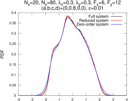
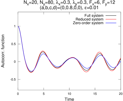
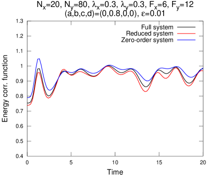
Fig. 1: Probability density functions, time autocorrelations, cross-correlations and energy autocorrelations. Parameters: $(a,b,c,d)=(0,0.8,0,0)$.

In this section we test the regimes with single type coupling (one of the constants $a,b,c,d$ is nonzero, and the rest are zero). In this section, we only test the regimes with nonzero constants $b,c,d$, as the single type coupling regime with $a\neq 0$ corresponds to the model previously studied in [4].

4.1.1 Regime with $(a,b,c,d)=(0,\pm 0.8,0,0)$

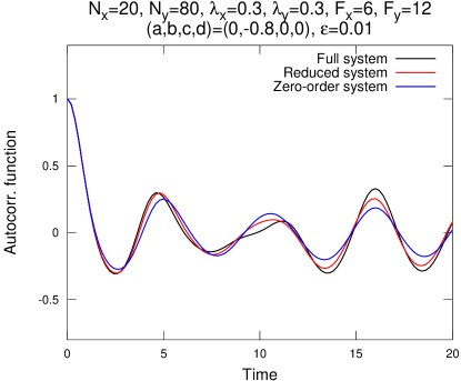
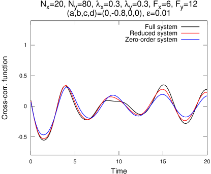
Fig. 2: Probability density functions, time autocorrelations, cross-correlations and energy autocorrelations. Parameters: $(a,b,c,d)=(0,-0.8,0,0)$.

$F_{x}=6$, $F_{y}=12$, $\lambda_{x}=\lambda_{y}=0.3$

$(a,b,c,d)=(0,0.8,0,0)$ $(a,b,c,d)=(0,-0.8,0,0)$ Reduced Zero-order PDF $3.103\cdot 10^{-3}$ $6.61\cdot 10^{-3}$ Corr. $4.13\cdot 10^{-2}$ $7.008\cdot 10^{-2}$ C-corr. $5.16\cdot 10^{-2}$ $8.721\cdot 10^{-2}$ K-corr. $7.695\cdot 10^{-3}$ $1.29\cdot 10^{-2}$ Reduced Zero-order PDF $6.471\cdot 10^{-3}$ $1.473\cdot 10^{-2}$ Corr. $5.877\cdot 10^{-2}$ $0.118$ C-corr. $7.009\cdot 10^{-2}$ $0.1415$ K-corr. $9.033\cdot 10^{-3}$ $2.384\cdot 10^{-2}$

Table 1: $L_{2}$-errors between the statistics of the slow variables of the full two-scale Lorenz model and the two reduced models, with $(a,b,c,d)=(0,\pm 0.8,0,0)$. Notations: “Reduced” stands for the reduced model from (6) and (11), and “Zero-order” stands for the poor man’s version of the reduced model, with linear approximations for $\bar{\boldsymbol{z}}(\boldsymbol{x})$ and $\boldsymbol{\Sigma}(\boldsymbol{x})$ replaced by constant mean values $\bar{\boldsymbol{z}}^{*}$ and $\boldsymbol{\Sigma}^{*}$.

Here we test the regimes with $b=\pm 0.8$, and $a=c=d=0$. This regime corresponds to bilinear multiplicative coupling in the slow variables, and quadratic additive coupling in the fast variables. The probability density functions, time autocorrelation, cross-correlation, and energy correlation functions are shown in Figures 1 and 2, while the $L_{2}$-errors between the curves are shown in Table 1. There is little difference between the plots, which means that the fast mean state $\boldsymbol{\bar{z}}(\boldsymbol{x})$ and $\boldsymbol{\Sigma}(\boldsymbol{x})$ are not very sensitive to changes in $\boldsymbol{x}$ for this type of coupling. Yet, one can see that the reduced model with linear correction for $\boldsymbol{\bar{z}}(\boldsymbol{x})$ and $\boldsymbol{\Sigma}(\boldsymbol{x})$ more precisely captures statistics of the full scale model, than the zero-order reduced model with fast mean state and covariance fixed at $\boldsymbol{\bar{z}}^{*}$ and $\boldsymbol{\Sigma}^{*}$ (see Table 1). Additionally, it appears that there is a weak effect of chaos suppression for this type of coupling regardless of the sign of $b$ (for both negative and positive $b$, the statistics of the coupled model show somewhat slower decay of autocorrelations and cross-correlations, and more sub-Gaussian energy correlation functions).

4.1.2 Regime with $(a,b,c,d)=(0,0,\pm 0.3,0)$

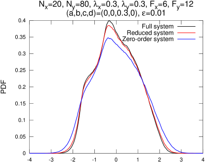
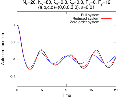
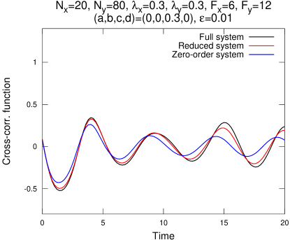
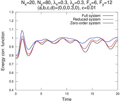
Fig. 3: Probability density functions, time autocorrelations, cross-correlations and energy autocorrelations. Parameters: $(a,b,c,d)=(0,0,0.3,0)$.

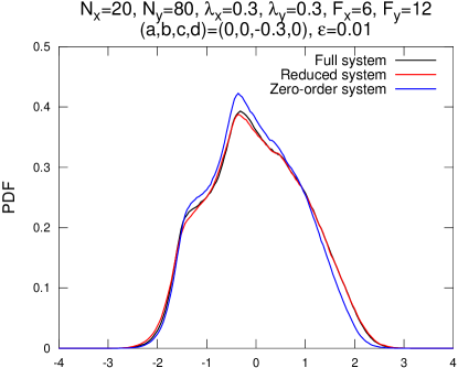
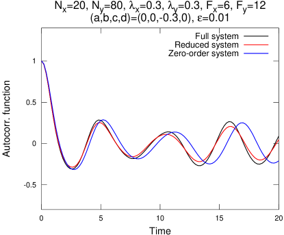
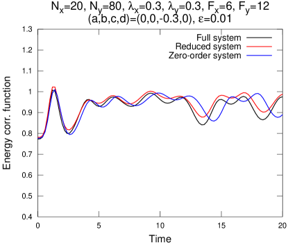
Fig. 4: Probability density functions, time autocorrelations, cross-correlations and energy autocorrelations. Parameters: $(a,b,c,d)=(0,0,-0.3,0)$.

Here we test the regimes with $c=\pm 0.3$, and $a=b=d=0$. This regime corresponds to quadratic additive coupling in the slow variables, and bilinear multiplicative coupling in the fast variables. The probability density functions, time autocorrelation, cross-correlation, and energy correlation functions are shown in Figures 3 and 4, while the $L_{2}$-errors between the curves are shown in Table 2. Like in the previous case, there is little difference between the plots, which means that the fast mean state $\boldsymbol{\bar{z}}(\boldsymbol{x})$ and $\boldsymbol{\Sigma}(\boldsymbol{x})$ are not very sensitive to changes in $\boldsymbol{x}$ for this type of coupling. Yet, one can see that the reduced model with linear correction for $\boldsymbol{\bar{z}}(\boldsymbol{x})$ and $\boldsymbol{\Sigma}(\boldsymbol{x})$ more precisely captures statistics of the full scale model, than the zero-order reduced model with fast mean state and covariance fixed at $\boldsymbol{\bar{z}}^{*}$ and $\boldsymbol{\Sigma}^{*}$ (see Table 2). Additionally, it appears that there is a weak effect of chaos suppression for this type of coupling for positive value of $c=0.3$ (the statistics of the coupled model show somewhat slower decay of autocorrelations and cross-correlations, and more sub-Gaussian energy correlation). No such effect is observed for the negative value $c=-0.3$.

$F_{x}=6$, $F_{y}=12$, $\lambda_{x}=\lambda_{y}=0.3$

$(a,b,c,d)=(0,0,0.3,0)$ $(a,b,c,d)=(0,0,-0.3,0)$ Reduced Zero-order PDF $5.49\cdot 10^{-3}$ $2.314\cdot 10^{-2}$ Corr. $5.559\cdot 10^{-2}$ $0.1788$ C-corr. $6.265\cdot 10^{-2}$ $0.2055$ K-corr. $9.605\cdot 10^{-3}$ $2.659\cdot 10^{-2}$ Reduced Zero-order PDF $3.707\cdot 10^{-3}$ $1.447\cdot 10^{-2}$ Corr. $5.238\cdot 10^{-2}$ $0.2399$ C-corr. $6.271\cdot 10^{-2}$ $0.2845$ K-corr. $9.62\cdot 10^{-3}$ $2.041\cdot 10^{-2}$

Table 2: $L_{2}$-errors between the statistics of the slow variables of the full two-scale Lorenz model and the two reduced models, with $(a,b,c,d)=(0,0,\pm 0.3,0)$. Notations: “Reduced” stands for the reduced model from (6) and (11), and “Zero-order” stands for the poor man’s version of the reduced model, with linear approximations for $\bar{\boldsymbol{z}}(\boldsymbol{x})$ and $\boldsymbol{\Sigma}(\boldsymbol{x})$ replaced by constant mean values $\bar{\boldsymbol{z}}^{*}$ and $\boldsymbol{\Sigma}^{*}$.

4.1.3 Regime with $(a,b,c,d)=(0,0,0,\pm 0.3)$

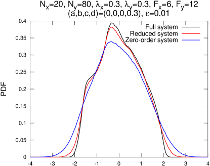
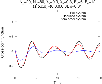
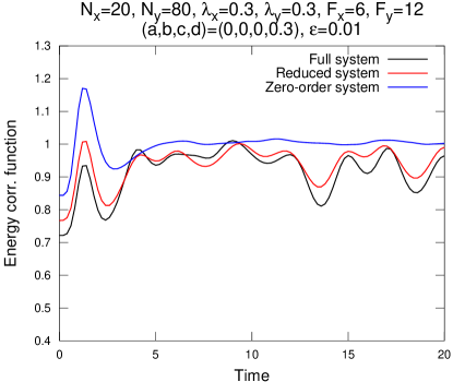
Fig. 5: Probability density functions, time autocorrelations, cross-correlations and energy autocorrelations. Parameters: $(a,b,c,d)=(0,0,0,0.3)$.

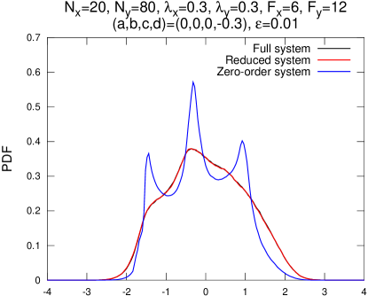
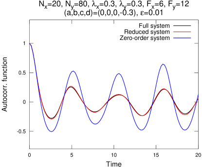
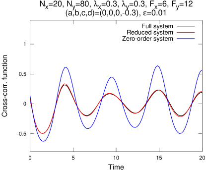
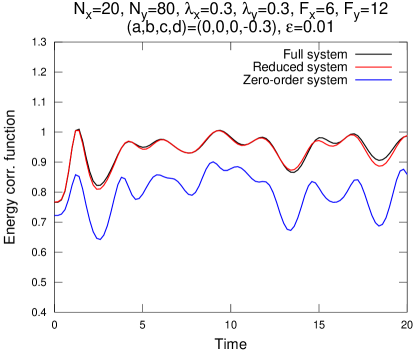
Fig. 6: Probability density functions, time autocorrelations, cross-correlations and energy autocorrelations. Parameters: $(a,b,c,d)=(0,0,0,-0.3)$.

Here we test the regimes with $c=\pm 0.3$, and $a=b=d=0$. This regime corresponds to quadratic multiplicative coupling in both the slow and fast variables. The probability density functions, time autocorrelation, cross-correlation, and energy correlation functions are shown in Figures 5 and 6, while the $L_{2}$-errors between the curves are shown in Table 3. Unlike previous cases, there is a significant difference between the results of the full two-scale/first-order reduced model, and the zero-order reduced model, which means that the fast mean state $\boldsymbol{\bar{z}}(\boldsymbol{x})$ and $\boldsymbol{\Sigma}(\boldsymbol{x})$ are sensitive to changes in $\boldsymbol{x}$ for this type of coupling. Similar to the previous cases, one can see that the reduced model with linear correction for $\boldsymbol{\bar{z}}(\boldsymbol{x})$ and $\boldsymbol{\Sigma}(\boldsymbol{x})$ more precisely captures the statistics of the full two-scale model, than the zero-order reduced model with fast mean state and covariance fixed at $\boldsymbol{\bar{z}}^{*}$ and $\boldsymbol{\Sigma}^{*}$ (see Table 3). Unlike previous types of coupling, here the chaos suppression or amplification depends on the sign of the constant $d$. For the positive value $d=0.3$, the coupled dynamics and the reduced model are clearly less chaotic and mixing than the zero-order reduced model with fast mean state and covariance fixed at $\boldsymbol{\bar{z}}^{*}$ and $\boldsymbol{\Sigma}^{*}$, which follows from the difference in decay of the correlation functions. The opposite effect is observed for the negative value $d=-0.3$. In particular, observe that the PDF of the zero-order reduced model displays three peaks for $d=-0.3$ (which is a sign of quasi-periodic motion), while the PDFs of both the two-scale Lorenz model and reduced models are unimodal.

$F_{x}=6$, $F_{y}=12$, $\lambda_{x}=\lambda_{y}=0.3$

$(a,b,c,d)=(0,0,0,0.3)$ $(a,b,c,d)=(0,0,0,-0.3)$ Reduced Zero-order PDF $1.012\cdot 10^{-2}$ $2.935\cdot 10^{-2}$ Corr. $7.397\cdot 10^{-2}$ $0.2638$ C-corr. $9.183\cdot 10^{-2}$ $0.3196$ K-corr. $1.632\cdot 10^{-2}$ $5.002\cdot 10^{-2}$ Reduced Zero-order PDF $1.342\cdot 10^{-3}$ $5.272\cdot 10^{-2}$ Corr. $1.923\cdot 10^{-2}$ $0.3881$ C-corr. $2.497\cdot 10^{-2}$ $0.4624$ K-corr. $3.656\cdot 10^{-3}$ $6.977\cdot 10^{-2}$

Table 3: $L_{2}$-errors between the statistics of the slow variables of the full two-scale Lorenz model and the two reduced models, with $(a,b,c,d)=(0,0,0,\pm 0.3)$. Notations: “Reduced” stands for the reduced model from (6) and (11), and “Zero-order” stands for the poor man’s version of the reduced model, with linear approximations for $\bar{\boldsymbol{z}}(\boldsymbol{x})$ and $\boldsymbol{\Sigma}(\boldsymbol{x})$ replaced by constant mean values $\bar{\boldsymbol{z}}^{*}$ and $\boldsymbol{\Sigma}^{*}$.

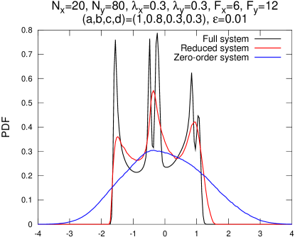
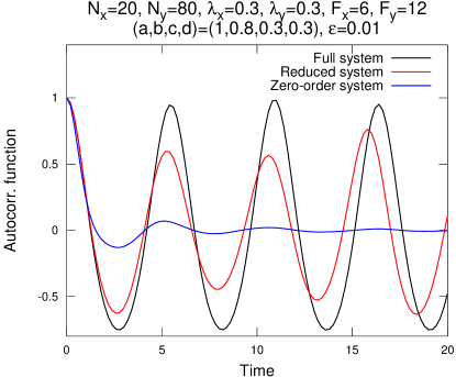
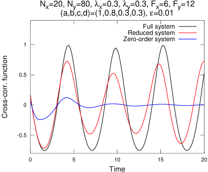
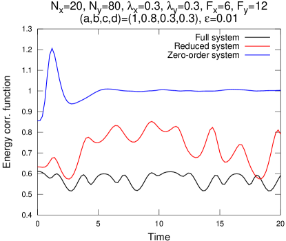
Fig. 7: Probability density functions, time autocorrelations, cross-correlations and energy autocorrelations. Parameters: $(a,b,c,d)=(1,0.8,0.3,0.3)$.

4.2 Combined coupling

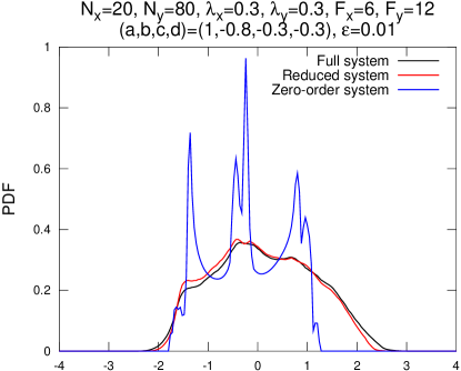
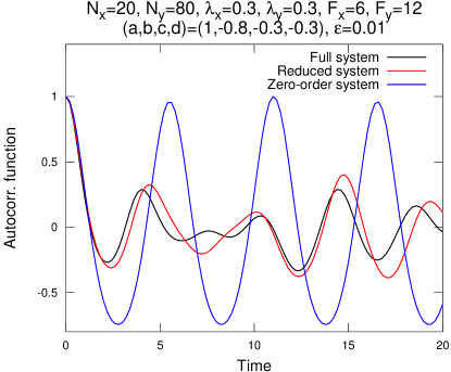
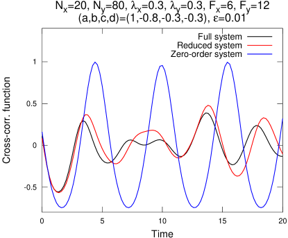
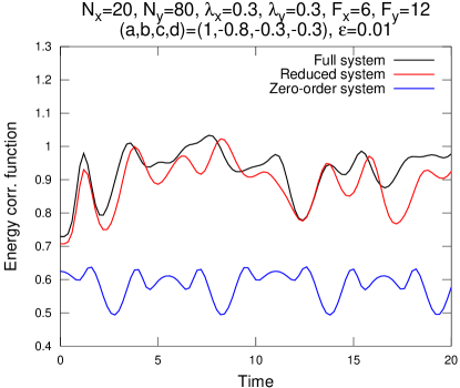
Fig. 8: Probability density functions, time autocorrelations, cross-correlations and energy autocorrelations. Parameters: $(a,b,c,d)=(1,-0.8,-0.3,-0.3)$.

In this section we test the regimes with all types of coupling observed previously in Section 4.1, combined together in the Lorenz model. In addition, the linear coupling is also switched on by setting $a=1$. Here we study the sets of parameters $(a,b,c,d)=(1,\pm 0.8,\pm 0.3,\pm 0.3)$. The probability density functions, time autocorrelation, cross-correlation, and energy correlation functions are shown in Figures 7 and 8, while the $L_{2}$-errors between the curves are shown in Table 4. It turns out that when all types of coupling are combined together there is a major difference between the two-scale/first-order reduced models, and the zero-order reduced model with fast mean state and covariance fixed at $\boldsymbol{\bar{z}}^{*}$ and $\boldsymbol{\Sigma}^{*}$, which means that the fast mean state $\boldsymbol{\bar{z}}(\boldsymbol{x})$ and $\boldsymbol{\Sigma}(\boldsymbol{x})$ are quite sensitive to changes in $\boldsymbol{x}$. Similar to the previous cases, here one can see that the reduced model with linear correction for $\boldsymbol{\bar{z}}(\boldsymbol{x})$ and $\boldsymbol{\Sigma}(\boldsymbol{x})$ much more precisely captures statistics of the full two-scale scale model, than the zero-order reduced model (see Table 3). Here the chaos suppression or amplification depends on the signs of the constant $b$, $c$ and $d$. For positive values of these constants, the coupled dynamics and the reduced model are clearly less chaotic and mixing than the zero-order reduced model, which follows from the difference in decay of the correlation functions. The opposite effect is observed for negative values of $b$, $c$ and $d$. In particular, observe that the PDF of the zero-order reduced model displays three strong peaks for $d=-0.3$ (which is a sign of quasi-periodic motion), while the PDFs of both the two-scale Lorenz model and reduced models are unimodal. On the contrary, for $d=0.3$ the PDF of the two-scale Lorenz model displays three peaks, which are roughly captured by the reduced model, while the zero-order reduced model produces nearly Gaussian PDF.

$F_{x}=6$, $F_{y}=12$, $\lambda_{x}=\lambda_{y}=0.3$

$(a,b,c,d)=(1,0.8,0.3,0.3)$ $(a,b,c,d)=(1,-0.8,-0.3,-0.3)$ Reduced Zero-order PDF $6.837\cdot 10^{-2}$ $0.1121$ Corr. $0.2237$ $0.4083$ C-corr. $0.2322$ $0.4153$ K-corr. $0.134$ $0.3356$ Reduced Zero-order PDF $1.24\cdot 10^{-2}$ $0.1252$ Corr. $0.2181$ $1.209$ C-corr. $0.2477$ $1.337$ K-corr. $2.89\cdot 10^{-2}$ $0.1707$

Table 4: $L_{2}$-errors between the statistics of the slow variables of the full two-scale Lorenz model and the two reduced models, with $(a,b,c,d)=(1,\pm 0.8,\pm 0.3,\pm 0.3)$. Notations: “Reduced” stands for the reduced model from (6) and (11), and “Zero-order” stands for the poor man’s version of the reduced model, with linear approximations for $\bar{\boldsymbol{z}}(\boldsymbol{x})$ and $\boldsymbol{\Sigma}(\boldsymbol{x})$ replaced by constant mean values $\bar{\boldsymbol{z}}^{*}$ and $\boldsymbol{\Sigma}^{*}$.

5 Conclusions

In this work we develop a simple approach for approximation of multiscale dynamics with nonlinear and multiplicative coupling via a reduced model for slow variables alone. The method is based on the linear approximation of averaged coupling terms by means of the fluctuation-dissipation theorem, which is only requires a single computation of certain long-term statistics from the fast limiting system with the slow terms set as constant parameters. This work is a direct extension of [4] onto nonlinear and multiplicative coupling (the original method in [4] was developed for linear coupling in both slow and fast variables). We verify through the numerical simulations with the rescaled two-scale Lorenz 96 model [5, 4] that, with nonlinear and multiplicative coupling in both slow and fast variables, the new simple reduced model produces statistics which are consistent with those of the complete two-scale Lorenz model. In contrast, the “zero-order” reduced model with constant parameterization of fast variables in coupling terms fails to reproduce the same set of statistics with comparable precision. The method appears to be convenient for practical applications due to its explicit construction – it lacks unknown parameters which have to be determined implicitly by comparing the performance of the reduced model against the full multiscale dynamics.

Appendix A Detailed derivation of the closure terms for the mean state and covariance matrix

In order to derive the formulas for the linear responses of the mean and covariance of the fast variables, for convenience we first make a linear change of variables in the following way: we rewrite (10) as

$$\begin{split}\frac{\mathrm{d}\boldsymbol{q}}{\mathrm{d}\tau}=\boldsymbol{S}^{-1}\boldsymbol{g}(\boldsymbol{\bar{z}}^{*}+\boldsymbol{S}\boldsymbol{q})+\boldsymbol{S}^{-1}(\boldsymbol{H}^{*}+\delta\boldsymbol{H}(\boldsymbol{x}))\boldsymbol{S}\boldsymbol{q}+\\ +\boldsymbol{S}^{-1}(\boldsymbol{h}^{*}+\boldsymbol{H}^{*}\boldsymbol{\bar{z}}^{*}+\delta\boldsymbol{h}(\boldsymbol{x})+\delta\boldsymbol{H}(\boldsymbol{x})\boldsymbol{\bar{z}}^{*}),\end{split}$$ (19)

where $\boldsymbol{S}=\boldsymbol{\Sigma}^{*\frac{1}{2}}$, and $\boldsymbol{z}=\boldsymbol{\bar{z}}^{*}+\boldsymbol{S}\boldsymbol{q}$, that is, $\boldsymbol{q}$ is the fluctuation of $\boldsymbol{z}$ around $\boldsymbol{\bar{z}}^{*}$ with the identity covariance matrix. Changing notations, we obtain

$$\begin{split}\frac{\mathrm{d}\boldsymbol{q}}{\mathrm{d}\boldsymbol{\tau}}=\boldsymbol{S}^{-1}\boldsymbol{g}&(\boldsymbol{\bar{z}}^{*}+\boldsymbol{S}\boldsymbol{q})+(\boldsymbol{\hat{H}}^{*}+\delta\boldsymbol{\hat{H}}(\boldsymbol{x}))\boldsymbol{q}+\boldsymbol{\hat{h}}^{*}+\delta\boldsymbol{\hat{h}}(\boldsymbol{x}),\\ \boldsymbol{\hat{h}}^{*}&=\boldsymbol{S}^{-1}(\boldsymbol{h}^{*}+\boldsymbol{H}^{*}\boldsymbol{\bar{z}}^{*}),\quad\boldsymbol{\hat{H}}^{*}=\boldsymbol{S}^{-1}\boldsymbol{H}^{*}\boldsymbol{S},\\ \delta\boldsymbol{\hat{h}}(\boldsymbol{x})=\boldsymbol{S}^{-1}&(\delta\boldsymbol{h}(\boldsymbol{x})+\delta\boldsymbol{H}(\boldsymbol{x})\boldsymbol{\bar{z}}^{*}),\quad\delta\boldsymbol{\hat{H}}(\boldsymbol{x})=\boldsymbol{S}^{-1}\delta\boldsymbol{H}(\boldsymbol{x})\boldsymbol{S}.\end{split}$$ (20)

Here, we can consider (20) as a dynamical system perturbed by $\delta\boldsymbol{\hat{h}}$ and $\delta\boldsymbol{\hat{H}}$, which has zero mean state and identity covariance matrix in the unperturbed state, and use the FDT to estimate the linear response of the mean state $\langle\boldsymbol{q}\rangle$ and the covariance $\langle\boldsymbol{q}\boldsymbol{q}^{T}\rangle$ to these perturbations, which can later be mapped into the original coordinates via backward linear transformation. The linear responses of the mean state $\delta\langle\boldsymbol{q}\rangle$ and covariance $\delta\langle\boldsymbol{q}\boldsymbol{q}^{T}\rangle$ are given by, respectively,

$$\begin{split}\delta\langle\boldsymbol{q}\rangle_{i}=\boldsymbol{R}_{ij}^{\hat{h}\to\hat{\bar{z}}}\delta\boldsymbol{\hat{h}}_{j}+\boldsymbol{R}_{ijk}^{\hat{H}\to\hat{\bar{z}}}\delta\boldsymbol{\hat{H}}_{jk},\\ \delta\langle\boldsymbol{q}\boldsymbol{q}^{T}\rangle_{ij}=\boldsymbol{R}_{ijk}^{\hat{h}\to\hat{\Sigma}}\delta\boldsymbol{\hat{h}}_{k}+\boldsymbol{R}_{ijkl}^{\hat{H}\to\hat{\Sigma}}\delta\boldsymbol{\hat{H}}_{kl},\end{split}$$ (21)

where the linear response operators are given by

$$\boldsymbol{R}_{ij}^{\hat{h}\to\hat{\bar{z}}}=\int_{0}^{\infty}\int_{\mathbb{R}^{N_{y}}}\frac{\partial}{\partial q_{j}}(\phi^{s}\boldsymbol{q})_{i}\,\mathrm{d}\mu(\boldsymbol{q})\,\mathrm{d}s,$$ (22a)

$$\boldsymbol{R}_{ijk}^{\hat{H}\to\hat{\bar{z}}}=\int_{0}^{\infty}\int_{\mathbb{R}^{N_{y}}}\frac{\partial}{\partial q_{j}}(\phi^{s}\boldsymbol{q})_{i}q_{k}\,\mathrm{d}\mu(\boldsymbol{q})\,\mathrm{d}s,$$ (22b)

$$\boldsymbol{R}_{ijk}^{\hat{h}\to\hat{\Sigma}}=\int_{0}^{\infty}\int_{\mathbb{R}^{N_{y}}}\frac{\partial}{\partial q_{k}}(\phi^{s}\boldsymbol{q}\otimes\phi^{s}\boldsymbol{q})_{ij}\,\mathrm{d}\mu(\boldsymbol{q})\,\mathrm{d}s,$$ (22c)

$$\boldsymbol{R}_{ijkl}^{\hat{H}\to\hat{\Sigma}}=\int_{0}^{\infty}\int_{\mathbb{R}^{N_{y}}}\frac{\partial}{\partial q_{k}}(\phi^{s}\boldsymbol{q}\otimes\phi^{s}\boldsymbol{q})_{ij}q_{l}\,\mathrm{d}\mu(\boldsymbol{q})\,\mathrm{d}s,$$ (22d)

where $\phi^{s}$ is the flow generated by the unperturbed system in (20) with $\delta\hat{\boldsymbol{h}}$ and $\delta\hat{\boldsymbol{H}}$ set to zeros, and $\,\mathrm{d}\mu$ is its invariant measure [1, 2, 3, 5, 4, 7, 6, 8]. At this point, we are going to assume that $\mu$ has a Gaussian density with zero mean state and identity covariance matrix (so-called quasi-Gaussian FDT approximation, [4, 7, 6, 8, 18]). Then, after integrating by parts, the responses of the mean state and covariance can be computed as

$$\boldsymbol{R}_{ij}^{\hat{h}\to\hat{\bar{z}}}=\int_{0}^{\infty}\int_{\mathbb{R}^{N_{y}}}(\phi^{s}\boldsymbol{q})_{i}q_{j}\,\mathrm{d}\mu(\boldsymbol{q})\,\mathrm{d}s,$$ (23a)

$$\boldsymbol{R}_{ijk}^{\hat{H}\to\hat{\bar{z}}}=\int_{0}^{\infty}\int_{\mathbb{R}^{N_{y}}}(\phi^{s}\boldsymbol{q})_{i}q_{j}q_{k}\,\mathrm{d}\mu(\boldsymbol{z})\,\mathrm{d}s,$$ (23b)

$$\boldsymbol{R}_{ijk}^{\hat{h}\to\hat{\Sigma}}=\int_{0}^{\infty}\int_{\mathbb{R}^{N_{y}}}(\phi^{s}\boldsymbol{q}\otimes\phi^{s}\boldsymbol{q})_{ij}q_{k}\,\mathrm{d}\mu(\boldsymbol{z})\,\mathrm{d}s,$$ (23c)

$$\boldsymbol{R}_{ijkl}^{\hat{H}\to\hat{\Sigma}}=\int_{0}^{\infty}\left[\int_{\mathbb{R}^{N_{y}}}(\phi^{s}\boldsymbol{q}\otimes\phi^{s}\boldsymbol{q})_{ij}q_{k}q_{l}\,\mathrm{d}\mu(\boldsymbol{z})-\delta_{ij}\delta_{kl}\right]\,\mathrm{d}s.$$ (23d)

By replacing measure averages with time averages (under the ergodicity assumption), we obtain

$$\boldsymbol{R}_{ij}^{\hat{h}\to\hat{\bar{z}}}=\int_{0}^{\infty}\left[\lim_{r\to\infty}\frac{1}{r}\int_{0}^{r}q_{i}(t+s)q_{j}(t)\,\mathrm{d}t\right]\,\mathrm{d}s,$$ (24a)

$$\boldsymbol{R}_{ijk}^{\hat{H}\to\hat{\bar{z}}}=\int_{0}^{\infty}\left[\lim_{r\to\infty}\frac{1}{r}\int_{0}^{r}q_{i}(t+s)q_{j}(t)q_{k}(t)\,\mathrm{d}t\right]\,\mathrm{d}s,$$ (24b)

$$\boldsymbol{R}_{ijk}^{\hat{h}\to\hat{\Sigma}}=\int_{0}^{\infty}\left[\lim_{r\to\infty}\frac{1}{r}\int_{0}^{r}q_{i}(t+s)q_{j}(t+s)q_{k}(t)\,\mathrm{d}t\right]\,\mathrm{d}s,$$ (24c)

$$\boldsymbol{R}_{ijkl}^{\hat{H}\to\hat{\Sigma}}=\int_{0}^{\infty}\left[\lim_{r\to\infty}\frac{1}{r}\int_{0}^{r}q_{i}(t+s)q_{j}(t+s)q_{k}(t)q_{l}(t)\,\mathrm{d}t-\delta_{ij}\delta_{kl}\right]\,\mathrm{d}s.$$ (24d)

Returning back to the original response coordinates, we obtain

$$\boldsymbol{R}_{ij}^{\hat{h}\to\bar{z}}=\int_{0}^{\infty}\left[\lim_{r\to\infty}\frac{1}{r}\int_{0}^{r}(z_{i}(t+s)-\bar{z}^{*}_{i})q_{j}(t)\,\mathrm{d}t\right]\,\mathrm{d}s,$$ (25a)

$$\boldsymbol{R}_{ijk}^{\hat{H}\to\bar{z}}=\int_{0}^{\infty}\left[\lim_{r\to\infty}\frac{1}{r}\int_{0}^{r}(z_{i}(t+s)-\bar{z}^{*}_{i})q_{j}(t)q_{k}(t)\,\mathrm{d}t\right]\,\mathrm{d}s,$$ (25b)

$$\boldsymbol{R}_{ijk}^{\hat{h}\to\Sigma}=\int_{0}^{\infty}\left[\lim_{r\to\infty}\frac{1}{r}\int_{0}^{r}(z_{i}(t+s)-\bar{z}^{*}_{i})(z_{j}(t+s)-\bar{z}^{*}_{j})q_{k}(t)\,\mathrm{d}t\right]\,\mathrm{d}s,$$ (25c)

$$\begin{split}\boldsymbol{R}_{ijkl}^{\hat{H}\to\Sigma}=\int_{0}^{\infty}\bigg{[}\lim_{r\to\infty}\frac{1}{r}\int_{0}^{r}(z_{i}(t+s)-\bar{z}^{*}_{i})(z_{j}(t+s)-\bar{z}^{*}_{j})\times\\ \times q_{k}(t)q_{l}(t)\,\mathrm{d}t-\Sigma^{*}_{ij}\delta_{kl}\bigg{]}\,\mathrm{d}s.\end{split}$$ (25d)

Returning back to the original perturbation coordinates, we obtain

$$\boldsymbol{R}_{ij}^{h\to\bar{z}}=\int_{0}^{\infty}\left[\lim_{r\to\infty}\frac{1}{r}\int_{0}^{r}(z_{i}(t+s)-\bar{z}^{*}_{i})(z_{k}(t)-\bar{z}^{*}_{k})\,\mathrm{d}t\right]\,\mathrm{d}s\;\Sigma^{*-1}_{kj},$$ (26a)

$$\begin{split}\boldsymbol{R}_{ijk}^{H\to\bar{z}}=\int_{0}^{\infty}\bigg{[}\lim_{r\to\infty}\frac{1}{r}\int_{0}^{r}(z_{i}(t+s)-\bar{z}^{*}_{i})(z_{l}(t)-\bar{z}^{*}_{l})\times\\ \times(z_{k}(t)-\bar{z}^{*}_{k})\,\mathrm{d}t\bigg{]}\,\mathrm{d}s\;\Sigma^{*-1}_{lj},\end{split}$$ (26b)

$$\begin{split}\boldsymbol{R}_{ijk}^{h\to\Sigma}=\int_{0}^{\infty}\bigg{[}\lim_{r\to\infty}\frac{1}{r}\int_{0}^{r}(z_{i}(t+s)-\bar{z}^{*}_{i})(z_{j}(t+s)-\bar{z}^{*}_{j})\times\\ \times(z_{l}(t)-\bar{z}^{*}_{l})\,\mathrm{d}t\bigg{]}\,\mathrm{d}s\;\Sigma^{*-1}_{lk},\end{split}$$ (26c)

$$\begin{split}\boldsymbol{R}_{ijkl}^{H\to\Sigma}=\int_{0}^{\infty}\bigg{[}\lim_{r\to\infty}\frac{1}{r}\int_{0}^{r}(z_{i}(t+s)-\bar{z}^{*}_{i})(z_{j}(t+s)-\bar{z}^{*}_{j})\times\\ \times(z_{m}(t)-\bar{z}^{*}_{m})(z_{l}(t)-\bar{z}^{*}_{l})\,\mathrm{d}t\;\Sigma^{*-1}_{mk}-\Sigma^{*}_{ij}\delta_{kl}\bigg{]}\,\mathrm{d}s,\end{split}$$ (26d)

which is given above in (12).

Acknowledgments. The author is supported by the National Science Foundation CAREER grant DMS-0845760, and the Office of Naval Research grants N00014-09-0083 and 25-74200-F6607.

References

- [1] R. Abramov, Short-time linear response with reduced-rank tangent map, Chin. Ann. Math., 30B (2009), pp. 447–462.
- [2] , Approximate linear response for slow variables of deterministic or stochastic dynamics with time scale separation, J. Comput. Phys., 229 (2010), pp. 7739–7746.
- [3] , Improved linear response for stochastically driven systems, Front. Math. China, (2011). accepted.
- [4] , A simple linear response closure approximation for slow dynamics of a multiscale system with linear coupling, Multiscale Model. Simul., 10 (2012), pp. 28–47.
- [5] , Suppression of chaos at slow variables by rapidly mixing fast dynamics through linear energy-preserving coupling, Commun. Math. Sci., 10 (2012), pp. 595–624.
- [6] R. Abramov and A. Majda, Blended response algorithms for linear fluctuation-dissipation for complex nonlinear dynamical systems, Nonlinearity, 20 (2007), pp. 2793–2821.
- [7] , New approximations and tests of linear fluctuation-response for chaotic nonlinear forced-dissipative dynamical systems, J. Nonlin. Sci., 18 (2008), pp. 303–341.
- [8] , New algorithms for low frequency climate response, J. Atmos. Sci., 66 (2009), pp. 286–309.
- [9] , Low frequency climate response of quasigeostrophic wind-driven ocean circulation, J. Phys. Oceanogr., (2011). early online release.
- [10] R. Buizza, M. Miller, and T. Palmer, Stochastic representation of model uncertainty in the ECMWF Ensemble Prediction System, Q. J. R. Meteor. Soc., 125 (1999), pp. 2887–2908.
- [11] D. Crommelin and E. Vanden-Eijnden, Subgrid scale parameterization with conditional Markov chains, J. Atmos. Sci., 65 (2008), pp. 2661–2675.
- [12] J.-P. Eckmann and D. Ruelle, Ergodic theory of chaos and strange attractors, Rev. Mod. Phys., 57 (1985), pp. 617–656.
- [13] I. Fatkullin and E. Vanden-Eijnden, A computational strategy for multiscale systems with applications to Lorenz 96 model, J. Comp. Phys., 200 (2004), pp. 605–638.
- [14] C. Franzke, A. Majda, and E. Vanden-Eijnden, Low-order stochastic model reduction for a realistic barotropic model climate, J. Atmos. Sci., 62 (2005), pp. 1722–1745.
- [15] K. Hasselmann, Stochastic climate models, part I, theory, Tellus, 28 (1976), pp. 473–485.
- [16] E. Lorenz, Predictability: A problem partly solved, in Proceedings of the Seminar on Predictability, Shinfield Park, Reading, England, 1996, ECMWF.
- [17] E. Lorenz and K. Emanuel, Optimal sites for supplementary weather observations, J. Atmos. Sci., 55 (1998), pp. 399–414.
- [18] A. Majda, R. Abramov, and M. Grote, Information Theory and Stochastics for Multiscale Nonlinear Systems, vol. 25 of CRM Monograph Series of Centre de Recherches Mathématiques, Université de Montréal, American Mathematical Society, 2005. ISBN 0-8218-3843-1.
- [19] A. Majda, I. Timofeyev, and E. Vanden-Eijnden, Models for stochastic climate prediction, Proc. Natl. Acad. Sci., 96 (1999), pp. 14687–14691.
- [20] , A mathematical framework for stochastic climate models, Comm. Pure Appl. Math., 54 (2001), pp. 891–974.
- [21] , A priori tests of a stochastic mode reduction strategy, Physica D, 170 (2002), pp. 206–252.
- [22] , Systematic strategies for stochastic mode reduction in climate, J. Atmos. Sci., 60 (2003), pp. 1705–1722.
- [23] T. Palmer, A nonlinear dynamical perspective on model error: A proposal for nonlocal stochastic-dynamic parameterization in weather and climate prediction models, Q. J. R. Meteor. Soc., 127 (2001), pp. 279–304.
- [24] G. Papanicolaou, Introduction to the asymptotic analysis of stochastic equations, in Modern modeling of continuum phenomena, R. DiPrima, ed., vol. 16 of Lectures in Applied Mathematics, American Mathematical Society, 1977.
- [25] H. Risken, The Fokker-Planck Equation, Springer-Verlag, New York, 2nd ed., 1989.
- [26] D. Ruelle, A measure associated with Axiom A attractors, Amer. J. Math., 98 (1976), pp. 619–654.
- [27] , Differentiation of SRB states, Comm. Math. Phys., 187 (1997), pp. 227–241.
- [28] , General linear response formula in statistical mechanics, and the fluctuation-dissipation theorem far from equilibrium, Phys. Lett. A, 245 (1998), pp. 220–224.
- [29] E. Vanden-Eijnden, Numerical techniques for multiscale dynamical systems with stochastic effects, Comm. Math. Sci., 1 (2003), pp. 385–391.
- [30] V. Volosov, Averaging in systems of ordinary differential equations, Russian Math. Surveys, 17 (1962), pp. 1–126.
- [31] D. Wilks, Effects of stochastic parameterizations in the Lorenz ’96 system, Q. J. R. Meteorol. Soc., 131 (2005), pp. 389–407.
- [32] L.-S. Young, What are SRB measures, and which dynamical systems have them?, J. Stat. Phys., 108 (2002), pp. 733–754.