Star formation in metal-poor gas clouds

Abstract

Observations of molecular clouds in metal-poor environments typically find that they have much higher star formation rates than one would expect based on their observed CO luminosities and the molecular gas masses that are inferred from them. This finding can be understood if one assumes that the conversion factor between CO luminosity and H₂ mass is much larger in these low metallicity systems than in nearby molecular clouds. However, it is unclear whether this is the only factor at work, or whether the star formation rate of the clouds is directly sensitive to the metallicity of the gas.

To investigate this, we have performed numerical simulations of the coupled dynamical, chemical and thermal evolution of model clouds with metallicities ranging from $0.01\>{\rm Z_{\odot}}$ to ${\rm Z_{\odot}}$. We find that the star formation rate in our model clouds has little sensitivity to the metallicity. Reducing the metallicity of the gas by two orders of magnitude delays the onset of star formation in the clouds by no more than a cloud free-fall time and reduces the time-averaged star formation rate by at most a factor of two. On the other hand, the chemical state of the clouds is highly sensitive to the metallicity, and at the lowest metallicities, the clouds are completely dominated by atomic gas. Our results confirm that the CO-to-H₂ conversion factor in these systems depends strongly on the metallicity, but also show that the precise value is highly time-dependent, as the integrated CO luminosity of the most metal-poor clouds is dominated by emission from short-lived gravitationally collapsing regions. Finally, we find evidence that the star formation rate per unit H₂ mass increases with decreasing metallicity, owing to the much smaller H₂ fractions present in our low metallicity clouds.

1 Introduction

High resolution observations of the gas and young stars within nearby massive spiral galaxies have shown that there is a tight correlation between the surface density of star formation and the surface density of molecular gas within these galaxies (see e.g. Wong & Blitz, 2002; Leroy et al., 2008; Bigiel et al., 2008, 2011; Schruba et al., 2011). However, similar observations of the star formation rate and the molecular gas surface density in low-metallicity environments, such as dwarf galaxies, tell a rather different story. Carbon monoxide (CO), the most commonly-used tracer of molecular gas, is difficult to detect in low metallicity gas, and even when detected, the ratio of the observed star formation rate to the CO luminosity is much larger than in higher metallicity regions (see e.g. Taylor, Kobulnicky & Skillman, 1998; Leroy et al., 2007; Schruba et al., 2011, 2012). If one assumes that the conversion factor between CO luminosity and H₂ mass – the so-called ‘X-factor’ – is the same in these systems as in the Milky Way, then these observations imply that there is a much larger amount of star formation per unit of molecular gas in low metallicity regions than in the Milky Way. Observations of larger “main-sequence” star-forming galaxies at $z>1$ by Genzel et al. (2012) also show that the ratio of the star-formation rate to the CO luminosity increases with decreasing metallicity, leading to a similar conclusion.

These results are the opposite of what one would naively expect, given the crucial role that metals and dust play in regulating the temperature of star-forming clouds in the local ISM. If, as is widely believed, the presence of large amounts of cold gas is a prerequisite for star formation, then one would expect star formation to become less effective as the metallicity is reduced, owing to the loss of coolants from the gas, as well as the reduced effectiveness of dust shielding. Indeed, recent work by Krumholz & Dekel (2012) has shown that galaxy formation models in which the star formation efficiency decreases with decreasing metallicity do a much better job of describing the specific star formation rates of high redshift galaxies than models in which the star formation rate is independent of metallicity.

One way to avoid this apparent contradiction is to adopt an X-factor with a strong dependence on metallicity. In this picture, one assumes that the CO luminosity per unit H₂ mass in low-metallicity environments is much smaller than in the Milky Way, implying that the actual reservoir of molecular gas present in such regions is much larger than one would predict from applying the Galactic X-factor to the observed CO emission. In other words, rather than having anomalously large star formation efficiencies, low metallicity dwarf galaxies and other similar systems may simply be strongly deficient in CO. This idea has considerable theoretical support from numerical models of the dependence of the X-factor on metallicity (see e.g. Bell et al., 2006; Glover & Mac Low, 2011; Narayanan et al., 2012; Feldmann, Gnedin, & Kravtsov, 2012), and also some observational support from direct measurements of the X-factor in the low metallicity environment of the Small Magellanic Cloud (Leroy et al., 2008; Bolatto et al., 2011).

If this model is correct, then it implies that the observations are not giving us an accurate picture of the relationship between the gas surface density and the star formation rate in these low-metallicity systems, and that the question of the star formation efficiency of the gas remains unresolved. Therefore, in order to explore the extent to which the star formation rate within a typical gravitationally-bound molecular cloud depends on the metallicity of the cloud, we have performed a series of numerical simulations of the chemical, thermal and dynamical evolution of model clouds with a wide range of metallicities. The layout of the remainder of our paper is as follows. In Section 2, we describe the approach used for our numerical simulations and the initial conditions that we adopt. In Section 3, we present our main results, and in Section 4, we discuss what these results imply regarding the dependence of the star formation rate on metallicity. Finally, we give our conclusions in Section 5.

2 Simulations

2.1 Numerical method

The simulations described in this paper were performed using a modified version of the Gadget 2 smoothed particle hydrodynamics (SPH) code (Springel, 2005). Our modifications include a sink particle algorithm for treating gravitationally collapsing regions that become too small to resolve (Bate, Bonnell & Price, 1995), the inclusion into the equation of motion of an optional confining pressure term (Benz, 1990), a treatment of gas-phase chemistry (described in more detail below), as well as radiative heating and cooling from a number of atomic and molecular species (Glover & Jappsen, 2007; Glover et al., 2010; Glover & Clark, 2012a), and an approximate treatment of the attenuation of the Galactic interstellar radiation field (ISRF). The effects of magnetic fields are not included.

Our treatment of the gas-phase chemistry combines the hydrogen chemistry network introduced in Glover & Mac Low (2007a, b) with the treatment of CO formation and destruction proposed by Nelson & Langer (1999). This combined network was tested against other simplified chemical networks for CO formation and destruction by Glover & Clark (2012a), who showed that it does a very good job of reproducing the results of more complex networks (e.g. Glover et al. 2010) for C⁺, C and CO, while incurring only one-third of the computational cost. Our treatment of H₂ formation on dust grains follows that of Hollenbach & McKee (1979), but we have verified that in the conditions studied in this paper, we would get very similar results if we were to use a more modern treatment such as that in Cazaux & Tielens (2004) and Cazaux & Spaans (2004). Further details regarding our treatment of the chemistry can be found in Glover & Clark (2012a). Note that the simulations presented in this paper do not include the effects of the freeze-out of CO onto dust grains. In Galactic star-forming clouds, CO freeze-out has been shown to have only a very minor effect on the thermal balance of the gas (Goldsmith, 2001), and we expect it to be even less important in lower metallicity clouds, as the dust temperatures in these clouds will generally be somewhat higher than in the typical Galactic case.

We assume in the majority of our simulations that our clouds are illuminated by the standard interstellar radiation field (ISRF), as parameterized by Draine (1978) in the ultraviolet and by Black (1994) at longer wavelengths. The effects of varying the strength of the ISRF are examined in Section 3.6.1. To treat dust extinction, H₂ self-shielding, CO self-shielding and the shielding of CO by H₂, we use the treecol algorithm (Clark, Glover & Klessen, 2012), as described in Glover & Clark (2012b). This algorithm provides us with an approximate 4$\pi$ steradian map of the column densities of hydrogen nuclei, H₂ and CO seen by each SPH particle, discretized into 48 equal-area pixels. To convert from the hydrogen column density to the dust extinction, we use the relationship $A_{\rm V}=5.348\times 10^{-22}(N_{\rm H,tot}/1\>{\rm cm^{-2}})({\rm Z}/{\rm Z_{\odot}})$ (Bohlin, Savage & Drake, 1978; Draine & Bertoldi, 1996), where we have assumed that the extinction scales linearly with the total metallicity. To convert from the H₂ and CO column densities to the shielding factors due to H₂ self-shielding, CO self-shielding and the shielding of CO by H₂, we use conversion factors from Draine & Bertoldi (1996) for H₂ self-shielding and Lee et al. (1996) for the other two terms.

2.2 Initial conditions

The initial state of our cloud is a uniform sphere with a total mass of 10${}^{4}\rm{M}_{\odot}$ and an initial hydrogen nuclei number density $n=300\>{\rm cm}^{-3}$, giving it an initial radius of approximately 6 pc. This cloud mass is typical of a small, nearby molecular cloud, such as e.g. the Perseus or Taurus molecular clouds. We have chosen to focus on the behaviour of a relatively small molecular cloud for two main reasons. First, it is simpler to simulate a small cloud with the required mass resolution than it would be to simulate a much larger cloud, since the required number of SPH particles scales linearly with the cloud mass. Second, a small molecular cloud will typically have a larger ratio of thermal to gravitational energy than a larger cloud, and so it is reasonable to expect that varying the metallicity will have more influence on the star formation rate in a small cloud than in a large one. We show in Section 3.1 below that large variations in the metallicity have only a small effect on the star formation rate, and because we are focussing on the case where we expect the metallicity variations to have the greatest effect, we can reasonably conclude that they will have even less effect in larger molecular clouds.

To model the gas making up the cloud, we use two million SPH particles, giving us a particle mass of $0.005\>{\rm M_{\odot}}$ and a mass resolution of $0.5\>{\rm M_{\odot}}$. We showed in Glover & Clark (2012b) that this mass resolution is sufficient to accurately determine the star formation rate, but that it does not allow us to draw strong conclusions regarding the form of the low-mass end of the stellar initial mass function. We inject bulk (non-thermal) motions into the cloud by imposing a turbulent velocity field that has a initial power spectrum $P(k)\propto k^{-4}$, where $k$ is the wavenumber. The energy in the turbulence is initially equal to the gravitational energy in the cloud, meaning that the initial root mean squared turbulent velocity is around 3 km s^-1. During the simulation, the turbulence is allowed to freely decay via shocks and compression-triggered cooling. We set the initial gas temperature to 20 K and the initial dust temperature to 10 K, but these values both alter rapidly once the simulation begins, as the gas and dust relax towards thermal equilibrium.

We consider five different metallicities in this study: ${\rm Z}=0.01,0.03,0.1,0.3,$ and $1.0\>{\rm Z_{\odot}}$. In our solar metallicity runs, we adopt the values $x_{\rm C}=1.4\times 10^{-4}$ and $x_{\rm O}=3.2\times 10^{-4}$ for our total oxygen and carbon abundances relative to hydrogen (Sembach et al., 2000). In the lower metallicity runs, we assume that $x_{\rm C}$ and $x_{\rm O}$ scale linearly with the metallicity. We also assume that our dust abundance scales linearly with ${\rm Z}$, but for simplicity assume that its properties remain the same (i.e. we do not change the form of the extinction curve as we move to lower ${\rm Z}$, merely the overall normalization). In every simulation, we assume that all of the available carbon starts in the form of C⁺ and that all of the available oxygen starts in neutral atomic form. For each metallicity, we perform two simulations, one in which the hydrogen is initially fully molecular, and a second in which it is initially fully atomic. We denote the simulations that start with molecular hydrogen by labels of the form Z$n$-M, where $n$ refers to the metallicity (e.g. Z1-M corresponds to solar metallicity, Z01-M to $0.1\>{\rm Z_{\odot}}$, etc.), while for the simulations starting with atomic hydrogen, we use labels of the form Z$n$-A.

Finally, we note that the cosmic ray ionization rate of atomic hydrogen in most of our simulated clouds was $\zeta_{\rm H}=10^{-17}\>{\rm s^{-1}}$. The cosmic ray ionization rates for the other major chemical species tracked in our chemical model were assumed to have the same ratio relative to the rate for atomic hydrogen as given in the UMIST99 chemical database (Le Teuff, Millar & Markwick, 2000). We explore the effects of varying $\zeta_{\rm H}$ in Section 3.6.2.

3 Results

3.1 Star formation rate

We first examine how the star formation rate in our model clouds varies as we vary the metallicity. As in Glover & Clark (2012b), we use the total mass of gas incorporated into sink particles as a proxy for the mass of stars formed. Although the limited mass resolution of our simulations means that the total number of sinks formed is probably not well-resolved, we have shown in previous work that our adopted resolution is sufficient to accurately determine the star formation rate (Glover & Clark, 2012b).

In the upper panel of Figure 1, we show how the mass in sinks varies with time in the five runs in which the hydrogen starts in the form of H₂, i.e. runs Z1-M, Z03-M, Z01-M, Z003-M and Z001-M. In run Z1-M, the solar metallicity run, the first sink forms at $t_{\rm SF}=2.21\>{\rm Myr}$. For comparison, the free-fall time of the cloud at its initial mean density is slightly longer, $t_{\rm ff}\sim 2.5\>{\rm Myr}$. However, the turbulence in the cloud creates overdense regions that are able to collapse more rapidly than the cloud as a whole, and so it is not particularly surprising that $t_{\rm SF}<t_{\rm ff}$. Once star formation has begun, it proceeds steadily, with the total mass of stars reaching $200\>{\rm M_{\odot}}$ after another 0.5 Myr (Table 1). Measured from the start of the simulation, the star formation efficiency per free-fall time of the cloud at this point is approximately 0.02, consistent with recent estimates of this quantity by Krumholz & Tan (2007) and Lada, Lombardi & Alves (2010). We halt the simulation shortly after this point because we do not include the effects of stellar feedback in our models and hence expect them to become increasingly inaccurate as the mass incorporated into stars increases, and as the individual stars approach the main sequence.

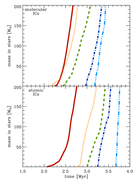
Figure 1: Upper panel: Mass in sinks, plotted as a function of time, for runs Z1-M (solid line), Z03-M (dotted line), Z01-M (dashed line), Z003-M (dot-dashed line) and Z001-M (dot-dot-dot-dashed line). In these runs, the hydrogen was initially in fully molecular form. Lower panel: The same quantity, but for runs Z1-A (solid line), Z03-A (dotted line), Z01-A (dashed line), Z003-A (dot-dashed line) and Z001-A (dot-dot-dot-dashed line). In these runs, the hydrogen was initially fully atomic.

Table 1: Star formation timescales in the different runs

Run	$t_{\rm SF}$ (Myr)	$t_{200}$ (Myr)
Z1-M	2.21	2.67
Z1-A	2.00	2.76
Z03-M	2.11	2.79
Z03-A	2.78	3.22
Z01-M	2.42	3.08
Z01-A	2.99	3.41
Z003-M	2.95	3.35
Z003-A	3.25	3.56
Z001-M	3.17	3.44
Z001-A	3.67	3.77

If we now look at what happens as we decrease the metallicity, we see that as we reduce Z, we delay the onset of star formation. The time at which the first sink particle forms, $t_{\rm SF}$, increases from 2.21 Myr in the solar metallicity case to 3.17 Myr in the $0.01\>{\rm Z_{\odot}}$ case. However, even in this case, the delay in the onset of star formation corresponds to considerably less than a cloud free-fall time, and star formation begins in all cases within 1.5 free-fall times. Moreover, once star formation begins, it proceeds at roughly the same rate in all five simulations.

The behaviour of the runs that start with fully atomic hydrogen is broadly similar. The onset of star formation in several of these simulations is delayed compared to the fully molecular case, but never by more than 0.6 Myr. The spread of values for $t_{\rm SF}$ is somewhat larger than in the molecular case, but remains less than a factor of two, and all of the model clouds have started forming stars within $1.5\>t_{\rm ff}$ after the beginning of the simulation. It is also interesting to note that once star formation has begun, it tends to proceed more rapidly in the low metallicity, initially atomic clouds than in the corresponding runs that start with molecular gas.

Taken together, these results demonstrate that even very large decreases in the metallicity of the gas have only a small effect on the ability of the cloud to form stars. Star formation is delayed for a short period in low metallicity gas compared to the solar metallicity case, but once star formation begins, it proceeds at roughly the same rate in all of the models, to within a factor of a few.

3.2 Chemical evolution

Although large changes in the metallicity of the gas have only a small effect on the ability of the cloud to form stars, they have a much larger effect on the chemistry of the gas. To quantify this, it is useful to look at how the mean abundances of various chemical species vary with time in the simulations. In our SPH simulations, the simplest mean abundance to examine is the mass-weighted mean, defined for a species $S$ as

$$\langle S\rangle_{\rm M}=\frac{1}{M}\sum_{i}m_{\rm i}x_{\rm S,i},$$ (1)

where $m_{i}$ is the mass of particle $i$, $x_{\rm S,i}$ is the fractional abundance of $S$ for particle $i$, $M$ is the total mass in the simulation and where we sum over all SPH particles that have not yet been accreted by sinks. In the case of H₂, using this definition would yield a value of 0.5 for fully molecular gas. This is not particularly intuitive and has the potential to cause confusion. Therefore, in this case alone, we use a slightly modified definition of the mean abundance which gives a value of 1.0 for fully molecular gas:

$$\langle{\rm H_{2}}\rangle_{\rm M}=\frac{1}{M}\sum_{i}2m_{\rm i}x_{\rm H_{2},i},$$ (2)

Table 2: Chemical state of the gas at the onset of star formation

Run	$F_{\rm H_{2}}$	$F_{\rm C^{+}}$	$F_{\rm C}$	$F_{\rm CO}$
Z1-M	0.883	0.601	0.084	0.315
Z1-A	0.599	0.664	0.146	0.190
Z03-M	0.779	0.906	0.030	0.064
Z03-A	0.304	0.896	0.036	0.068
Z01-M	0.598	0.978	0.009	0.013
Z01-A	0.0887	0.978	0.011	0.011
Z003-M	0.371	0.988	0.004	0.008
Z003-A	0.0191	0.990	0.004	0.006
Z001-M	0.2603	0.990	0.003	0.007
Z001-A	0.00775	0.990	0.003	0.007

Note: $F_{\rm H_{2}}$ is the fraction of the total amount of hydrogen in the form of H₂, while $F_{\rm C^{+}}$, $F_{\rm C}$ and $F_{\rm CO}$ are the fractions of the total available amount of carbon in the form of C⁺, C and CO, respectively.

3.2.1 Carbon monoxide (CO)

In Figure 2, we show how the mass-weighted mean abundance of CO varies with time in our simulations. At solar metallicity, our simulated clouds can form CO relatively easily. CO formation in the two solar metallicity runs occurs rapidly at the beginning of the simulation, but slows down significantly by $t\sim 1\>{\rm Myr}$, owing to the fact that by this point, most of the dense, well-shielded gas that can support a high CO fraction is already fully molecular, while the regions that remain primarily atomic have low equilibrium CO fractions. Nevertheless, the CO fraction does not settle into a steady state, owing to the global collapse of the cloud. This steadily increases the amount of dense, well-shielded gas that is available, and hence allows the CO fraction to continue to increase with time, albeit at a much slower rate.

Comparing runs Z1-M and Z1-A, we see that the initial state of the hydrogen has a pronounced influence on the CO fraction at early times. In run Z1-M, molecular hydrogen is immediately available to participate in the network of chemical reactions responsible for forming CO, allowing the CO fraction in the densest gas to increase very quickly once the simulation begins. In run Z1-A, on the other hand, CO formation can begin only once some H₂ has formed, and becomes efficient only once the H₂ fraction becomes large. The growth of the CO fraction in run Z1-A therefore lags behind that of the CO fraction in run Z1-M by about 0.5 Myr at early times.

As we reduce the metallicity of the clouds, it becomes much harder for them to form large amounts of CO. The mean CO abundance decreases far more rapidly with decreasing metallicity than would be expected simply from the reduction in the amount of carbon available. This is illustrated particularly clearly in Table 2, where we list the fraction of the total amount of carbon found in the form of C⁺, C and CO at the onset of star formation in the different runs. In the solar metallicity runs, between 20–30% of the carbon has been converted to CO at the point at which star formation begins. In the $0.3\>{\rm Z_{\odot}}$ runs, however, only 6–7% of the available carbon is found in the form of CO, while in the lower metallicity runs, the fraction is never larger than around 1.5%.

Another important point to note from Figure 2 is that in the lower metallicity runs, most of the CO that forms does so shortly before the onset of star formation. As we shall see later, the CO in these runs is concentrated in the same high-density gas that is responsible for forming the stars (see Section 3.3 below). Initially, very little of this gas exists, and the CO fraction is very small. Once a small sub-region of the cloud becomes gravitationally unstable and collapses, the amount of dense gas rapidly increases, as does the amount of CO present in the cloud (although the majority of the carbon remains in the form of C⁺; see Table 2).

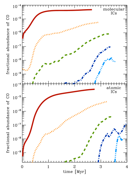
Figure 2: Upper panel: Evolution with time of the mass-weighted mean fractional abundance of CO for runs Z1-M, Z03-M, Z01-M, Z003-M and Z001-M. Lower panel: the same, but for runs Z1-A, Z03-A, Z01-A, Z003-A and Z001-A.

3.2.2 Molecular hydrogen (H₂)

Finally, it is interesting to examine how the H₂ fraction varies with time in our simulations. This is illustrated in Figure 3. In the runs that start with the hydrogen already in the form of H₂, we initially have more molecular gas than we would do if the cloud were in photodissociation equilibrium, and $\langle{\rm H_{2}}\rangle_{\rm M}$ therefore decreases with time. Although the photodissociation timescale for unshielded H₂ is short (less than 1000 yr), the high level of self-shielding provided by the H₂ and the additional attenuation of the incoming radiation provided by the dust act to substantially reduce the H₂ photodissociation rate within the cloud compared to its value in unshielded gas. This has the effect of dramatically lengthening the effective photodissociation timescale for most of the gas, with the result that the clouds do not have sufficient time to reach chemical equilibrium before they start forming stars. The amount of H₂ lost from the clouds depends on the metallicity. In the solar metallicity case, the cloud only loses a little of its H₂, while in the runs with $Z\leq 0.03\>{\rm Z_{\odot}}$, more than half of the initial molecular content is destroyed, and the clouds are dominated by atomic hydrogen by the time that they start forming stars.

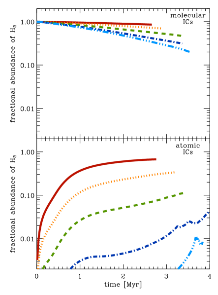
Figure 3: Upper panel: Evolution with time of the mass-weighted mean fractional abundance of H₂, for runs Z1-M, Z03-M, Z01-M, Z003-M and Z001-M. Lower panel: the same, but for runs Z1-A, Z03-A, Z01-A, Z003-A and Z001-A.

This sensitivity to metallicity is driven by a combination of effects. As we reduce the amount of dust in the gas, the mean extinction of the cloud decreases and so there is less attenuation of the incoming ultraviolet radiation. At the same time, the formation rate of H₂ also decreases, as this is directly dependent on the amount of dust present in the gas. In practice, it is the latter effect that appears to be more important, as demonstrated by the results from the runs that start with their hydrogen in atomic form. In these runs, we see a strong dependence of the H₂ fraction on metallicity. The solar metallicity run increases its mean H₂ fraction from zero to roughly 0.6 by the time it starts forming stars, in line with estimates from previous work (see e.g. Glover & Mac Low, 2007b; Glover & Clark, 2012b). However, as we reduce the metallicity, the increase in the H₂ formation timescale makes it much harder to produce large quantities of molecular gas even in regions that are well-shielded from the ultraviolet radiation field. As a result, the cloud remains dominated by atomic hydrogen in all of our runs with $Z=0.1\>{\rm Z_{\odot}}$ and below.

3.3 CO distribution at the onset of star formation

In Figure 4, we show how the CO abundance of the gas varies with density and temperature within our simulated clouds at a point just before the beginning of star formation. In every case, we see that at low densities, very little CO is present, while at high densities, most of the available carbon is in the form of CO. The density at which the transition between these two regimes occurs is a strong function of metallicity. In the solar metallicity case, it occurs at densities of around $n\sim 10^{3}\>{\rm cm^{-3}}$, although some gas with high CO fraction can be found at lower densities, and some higher density gas is seen to have a relatively low CO fraction. This is consistent with the idea that both the density and visual extinction of the gas must be high in order for it to have a high CO fraction, and with our previous finding that there is only a poor correlation between the local volume density and the visual extinction of gas within turbulent clouds (Glover et al., 2010). The clear correlation between the gas temperature and the CO abundance is also consistent with the extinction playing an important role: the gas with $T>20\>{\rm K}$ has a low visual extinction and consequently is heated efficiently by photoelectric emission from dust grains, while regions with $T<20\>{\rm K}$ typically have higher visual extinctions and hence are less affected by photoelectric heating.

As we move to lower metallicity, the density separating the low CO and high CO regimes systematically increases, evolving approximately as $n\propto{\rm Z^{-1}}$. This behaviour is again due to the dependence of the CO abundance on the extinction of the gas. As the metallicity decreases, a higher column density of gas is required in order to produce the same visual extinction, and the requisite column densities tend to only be found within denser regions of the flow. One important consequence of this behaviour is that the nature of the CO-rich regions changes as we move to lower metallicities. In the solar metallicity case, a density of $n\sim 10^{3}\>{\rm cm^{-3}}$ corresponds to an overdensity of only a factor of a few relative to the initial mean density of the cloud. Such an overdensity is easily produced simply by turbulent compression of the gas, without the need to invoke gravity, and much of the CO is located in overdense regions that are not self-gravitating. At lower metallicities, however, the required density becomes much higher and therefore much harder to reach simply through turbulent compression of the gas. Consequently, gravity begins to play more of a role, and the CO in the cloud becomes increasingly concentrated within strongly self-gravitating, collapsing regions. This naturally explains the strong time dependence in the CO abundance that we have already noted in Section 3.2.1.

The importance of gravitational collapse for producing the CO abundances that we find in our low metallicity simulations can also be clearly seen if we compare our results to those from Glover & Mac Low (2011). This earlier study considered CO formation in turbulent gas without self-gravity, and found that the mean CO abundance was highly sensitive to the mean visual extinction of the cloud, falling by almost five orders of magnitude as the mean extinction decreased from $\bar{A}_{\rm V}\sim 3$ to $\bar{A}_{\rm V}\sim 0.3$. If we consider our model clouds at an early time, say $t\sim 1\>{\rm Myr}$, when we expect the turbulent velocity field to have created significant amounts of dense sub-structure but when run-away gravitational collapse has not yet begun, then we find a similarly strong sensitivity to metallicity, particularly in the runs starting with atomic rather than molecular hydrogen. If we consider much later times, however, once gravitational collapse has begun in all of the models, then we see that the mean CO abundance becomes considerably less sensitive to the metallicity of the cloud.

3.4 Temperature distribution

The phase diagrams plotted in Figure 4 also show us how the temperature distributions of our simulated clouds vary with metallicity. In our solar metallicity clouds, we can see that there are three distinct regimes. At densities $n<10^{3}\>{\rm cm^{-3}}$, the cooling of the gas is dominated by C⁺ fine structure emission, while the heating is dominated by the photoelectric effect. The balance between these two processes yields a characteristic temperature that is a steeply decreasing function of the density, declining from $T\sim 100$ K at $n\sim 30\>{\rm cm^{-3}}$ to $T\sim 20$ K at $n\sim 1000\>{\rm cm^{-3}}$. At higher densities, $10^{3}<n<10^{5}\>{\rm cm^{-3}}$, there is considerable scatter in the temperature distribution. This scatter is due in large part to the fact that the dominant coolant in this regime is CO, and the effectiveness with which this can cool the gas depends to a large extent on the local optical depth of the CO $J=1\rightarrow 0$ rotational emission line (see also the discussion of this point in Glover & Clark, 2012b). In the run starting from initially atomic gas, an additional contribution to the scatter in this density regime comes from the influence of H₂ formation heating, which is responsible for the pronounced bulge in the distribution at $T\sim 20$–30 K and $n\sim 3\times 10^{4}\>{\rm cm^{-3}}$. Finally, at densities $n>10^{5}\>{\rm cm^{-3}}$, the scatter in the temperature distribution abruptly vanishes, as the gas temperature becomes strongly coupled to the dust temperature.

If we now examine what happens as we reduce the metallicity, we see that the temperature distribution tends to flatten. The temperature of the lowest density gas increases from roughly 100 K in the solar metallicity case to roughly 200–300 K in the ${\rm Z}=0.01\>{\rm Z_{\odot}}$ run, but the efficient cooling that the fine structure lines of C⁺ and O provide at these temperatures even in the low-metallicity runs prevents the temperature from rising much further. At the high density end of the distribution, however, the influence of metallicity is much more pronounced. The timescale on which energy is transferred between the gas and the dust scales with metallicity and density as $t_{\rm gd}\propto n^{-1}({\rm Z}/{\rm Z_{\odot}})^{-1}$, and the gas and dust temperatures become strongly coupled only once this timescale becomes shorter than the local dynamical time, which in this case is the free-fall time of the gas. Therefore, as Z decreases, the density at which the dust and gas temperatures become strongly coupled increases. Consequently, in the lower metallicity clouds, much of the dense gas must rely on CO cooling rather than dust cooling. However, CO cooling also becomes increasingly ineffective as we move to lower metallicities, as the CO abundance declines. On the other hand, the rate at which the dense gas is heated by the photoelectric effect increases as we decrease Z, owing to the consequent reduction in the mean extinction of the gas. The net effect is to increase the temperature of the densest gas from roughly 5 K in the solar metallicity case to anywhere between 50 K and 100 K in the ${\rm Z}=0.01\>{\rm Z_{\odot}}$ case. This increase in the temperature of the dense gas makes it much harder to create high density substructure within the cloud, whether through the action of turbulence or that of gravity, explaining why it takes longer for the cloud to start forming stars.

The increase in the gas temperature will also lead to an increase in the Jeans mass. If we compare the temperatures in the runs at a density of $10^{4}\>{\rm cm^{-3}}$, characteristic of most prestellar cores, then we see that there is roughly a factor of two increase in the temperature between the solar metallicity case and the $0.01\>{\rm Z_{\odot}}$ case, corresponding to an increase in the Jeans mass by about a factor of three. If we look at the densest gas in our simulations, we see an even stronger effect. The change in the Jeans mass that occurs as we reduce the metallicity could potentially have a pronounced influence on the initial mass function of the stars that form, although the limited mass resolution of our simulations does not allow us to address this issue with confidence. Nevertheless, it is important to realise that the Jeans mass in the dense gas remains much smaller than the mass of the cloud. Since the cloud itself also remains gravitationally bound in even the lowest metallicity run, the gravitational collapse of part or all of the gas within it, and the consequent formation of stars, is an inevitable outcome of the evolution of the cloud.

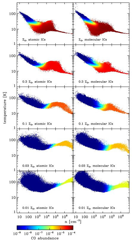
Figure 4: Phase diagram showing the temperature of the gas as a function of its density, colour-coded to indicate the CO abundance at each point in density-temperature space.

3.5 CO emission

The results of the previous sections demonstrate that the CO content of the low metallicity clouds is much smaller than the CO content of the solar metallicity clouds. It is therefore reasonable to assume that the lower metallicity clouds will produce much less emission in the $J=1\rightarrow 0$ rotational transition of ¹²CO, the most commonly used observational tracer of molecular gas. To confirm this expectation, we have computed emission maps for this transition for each of our model clouds using the RADMC-3D radiative transfer code.

In Figure 5, we show velocity-integrated emission maps of the central region of each of our model clouds at a point just before the onset of star formation. In each case, we have computed the emission arising from a cubic region of side length 16.2 pc centered on the cloud which was discretised onto a $128^{3}$ grid. The CO level populations were computed using the large velocity gradient (LVG) approximation, and we account for small-scale, unresolved motions by including a uniform microturbulent contribution $v_{\rm mtb}=0.2\>{\rm km}\>{\rm s^{-1}}$ to the line broadening. Further details of the operation of the code can be found in Shetty et al. (2011a, b).

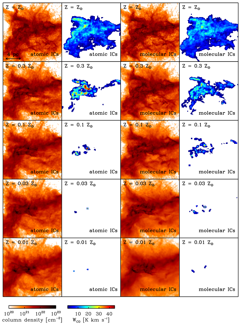
Figure 5: Maps of column density (first and third columns) and integrated intensity in the $J=1\rightarrow 0$ rotational transition of ¹²CO (second and fourth columns) for each of the simulations. The maps show a region of side length 16.2 pc that includes roughly 80% of the total cloud mass, but almost all of the CO emission. The CO integrated intensity maps were produced using the RADMC-3D radiative transfer code, as described in the text.

The emission maps in Figure 5 demonstrate that as we reduce the metallicity of the gas, the CO emission produced by the cloud does indeed decrease. The diffuse CO emission that traces the majority of the cloud volume in the solar metallicity runs is quickly lost as we move to lower metallicities, but the densest gas continues to produce distinct emission peaks down to very low metallicities. The peak value of the CO velocity-integrated intensity, $W_{\rm CO,max}$, does not show any clear dependence on the metallicity of the gas (Table 3), but the mean intensity, $W_{\rm CO,mean}$, decreases rapidly as the metallicity decreases. The mean intensity also tends to be smaller in the runs that start with atomic hydrogen rather than molecular hydrogen, although this is not a large effect in most of the runs.

We have also computed the mean X-factor for each region, using the following definition:

$$X_{\rm CO}=\frac{N_{\rm H_{2},mean}}{W_{\rm CO,mean}},$$ (3)

where $N_{\rm H_{2},mean}$ is the mean value of the H₂ column density. We list the resulting values in Table 3, in units of the canonical value for Galactic GMCs, X${}_{\rm CO,gal}=2\times 10^{20}\>{\rm cm^{-2}}\>({\rm K\>km\>s}^{-1})^{-1}$ (see e.g. Dame et al., 2001). We see that as we reduce the metallicity of the gas, X_CO increases, but that the strength of this effect depends on the initial chemical state of the gas. In the runs that start with their hydrogen in molecular form, the mean H₂ column density of the cloud remains large at low metallicities and X_CO shows a strong sensitivity to metallicity, driven by the substantial decrease in $W_{\rm CO,mean}$ that occurs at low Z. On the other hand, the low metallicity runs that start with their hydrogen in atomic form have much lower H₂ column densities than their higher metallicity counterparts, and hence show less variation in X_CO, as the reduction in $W_{\rm CO,mean}$ is offset by the reduction in the mean H₂ column density. The behaviour of real clouds probably lies somewhere between these two extreme cases.

Table 3: CO intensities and X_CO

Run	$W_{\rm CO,max}$	$W_{\rm CO,mean}$	XCO / XCO,gal
Z1-M	25.7	3.46	2.06
Z1-A	29.9	3.23	1.53
Z03-M	37.0	1.34	4.76
Z03-A	53.5	1.27	1.97
Z01-M	37.7	0.217	22.6
Z01-A	98.2	0.144	4.99
Z003-M	38.7	0.045	66.3
Z003-A	32.8	0.016	10.0
Z001-M	8.16	0.0068	306.7
Z001-A	25.6	0.0106	8.27

Note: $W_{\rm CO,max}$ is the maximum value of the CO velocity-integrated intensity, while $W_{\rm CO,mean}$ is the mean value, averaged over all of the lines of sight considered in the calculation. Both values have units of K km s^-1. X_CO is the mean conversion factor between CO intensity and H₂ mass, and X${}_{\rm CO,gal}=2\times 10^{20}\>{\rm cm^{-2}}\>({\rm K\>kms}^{-1})^{-1}$ is the canonical Galactic value of X_CO (Dame et al., 2001).

Another issue that should be borne in mind when considering how X_CO varies with metallicity is that the values that we obtain for our low metallicity clouds are highly time-dependent. The CO emission of these clouds is dominated by emission from a few dense, self-gravitating regions, and we would expect $W_{\rm CO,mean}$ for these clouds to be much lower if we were to observe them at an earlier time in their evolution, before the onset of gravitational collapse in these regions.

Looking at the column density projections of the clouds (also shown in Figure 5), we see that as we decrease the metallicity, the structure of the cloud changes. The gas becomes more centrally condensed as we decrease Z, and loses much of the substructure that is present in the solar metallicity run. This behaviour is a consequence of the higher gas temperatures found in the lower metallicity runs. A higher temperature implies a higher sound-speed and hence a lower Mach number for the turbulence, with the result that the turbulence is able to generate less structure in the density field (see e.g. Padoan, Nordlund & Jones, 1997; Passot & Vázquez-Semadeni, 1998; Price, Federrath & Brunt, 2011; Molina et al., 2012). It also leads to a higher characteristic Jeans mass, making it less likely that the overdense regions generated by the turbulence will be gravitationally bound.

3.6 Environmental sensitivity

The simulations that we have discussed in detail above were performed using only a single, fixed value for the strength of the interstellar radiation field and for the cosmic ray ionization rate. In reality, both of these values will vary somewhat from region to region within a galaxy, and from galaxy to galaxy. For example, we would expect the UV radiation field strength to be higher in a low metallicity dwarf galaxy than in a high metallicity spiral, given the same surface density of star formation in both systems, owing to the smaller amount of dust extinction in the lower metallicity system.

Therefore, in order to establish the extent to which the conclusions that we draw in this paper depend on our assumptions regarding the strength of the ISRF and the cosmic ray ionization rate, we have performed several simulations in which these values were varied. To prevent the number of simulations from becoming completely impractical, we considered only the two extreme cases where ${\rm Z=Z_{\odot}}$ and ${\rm Z}=0.01\>{\rm Z_{\odot}}$, and in both cases adopted molecular initial conditions. We performed simulations in which the strength of the ISRF was increased or decreased by a factor of ten (hereafter referred to with labels of the form Z$n$-G10 and Z$n$-G01, respectively, where $n$ denotes the metallicity, as before) and simulations in which $\zeta_{\rm H}$ was increased or decreased by a factor of ten (hereafter referred to with labels of the form Z$n$-CR10 and Z$n$-CR01, respectively). In the runs in which $\zeta_{\rm H}$ was varied, the other cosmic ray ionization rates were also varied so as to keep their ratios with $\zeta_{\rm H}$ unaltered.

In our present study, we do not explore the effect of more extreme changes in the radiation field strength or cosmic ray ionization rate, such as may be expected in starburst environments. We plan to address this issue in future work.

3.6.1 Effects of varying the strength of the ISRF

In the upper panel of Figure 6, we show how increasing or decreasing the strength of the interstellar radiation field affects the star formation rate in our model clouds. In the solar metallicity case, we see that changes in the strength of the ISRF have very little effect – all three of our model clouds begin forming stars at almost the same time, give-or-take 0.1 Myr. The fact that we do not see a strong dependence of the star formation rate on the strength of the ISRF in these runs is easy to understand, as in these clouds, gravitationally-bound pre-stellar cores form only in regions with high dust extinctions. The thermal state of the gas in the cores is therefore insensitive to changes in the strength of the ultraviolet portion of the ISRF, as UV photons do not penetrate into these regions. It is sensitive to changes in the mid-IR and far-IR portions of the ISRF, but in this case the dust temperature is only a very weak function of the radiation field strength. For the dust model adopted in our simulations, $T_{\rm d}\propto U_{\rm IR}^{1/6}$, where $U_{\rm IR}$ is the radiation energy density in the mid-IR and far-IR, and so changes of an order of magnitude in $U_{\rm IR}$ lead to at most a 50% change in the dust temperature, which is not enough to significantly affect the star formation process.

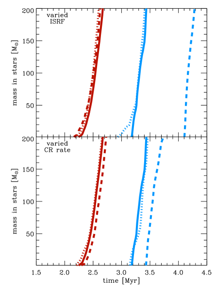
Figure 6: Upper panel: Mass in sinks, plotted as a function of time, for runs Z1-M (left-hand solid line), Z1-G01 (left-hand dotted line), Z1-G10 (left-hand dashed line), Z001-M (right-hand solid line), Z001-G01 (right-hand dotted line) and Z001-G10 (right-hand dashed line). Lower panel: The same quantity, but for runs Z1-M (left-hand solid line), Z1-CR01 (left-hand dotted line), Z1-CR10 (left-hand dashed line), Z001-M (right-hand solid line), Z001-CR01 (right-hand dotted line) and Z001-CR10 (right-hand dashed line).

In our ${\rm Z}=0.01\>{\rm Z_{\odot}}$ runs, the effect of changing the strength of the ISRF is more pronounced. Reducing the radiation field strength by an order of magnitude has little effect on the star formation rate, but increasing it by an order of magnitude delays the onset of star formation by almost $1\>{\rm Myr}$. However, once star formation begins in run Z001-G10, it proceeds at about the same rate as in the other runs.

In Table 4, we show how the chemical state of the gas at the onset of star formation varies as we vary the strength of the ISRF. In the solar metallicity runs, we see that although the fraction of the hydrogen that is in the form of H₂ decreases as we increase the radiation field strength, all three of our simulated clouds remain primarily molecular. The effect on the carbon chemistry is more pronounced, with the mass fraction of carbon in the form of CO, $F_{\rm CO}$, decreasing by around a factor of two for each factor of ten increase in the radiation field strength. The amount of C⁺ in the clouds also changes substantially, while the amount of atomic carbon changes by less than 50%.

Once again, however, changes in the radiation field strength have a much larger effect in the low metallicity runs than in the solar metallicity runs. Decreasing the strength of the field by a factor of ten dramatically reduces the amount of H₂ that is destroyed by photodissociation, meaning that the hydrogen in the cloud remains largely in molecular form at the onset of star formation. On the other hand, increasing the radiation field strength leads to an almost complete loss of H₂ from the gas. The effect on the CO is less pronounced, as the CO is concentrated in dense gas that is less susceptible to the effects of photodissociation, but even in this case we see a factor of two change in the CO mass fraction for each factor of ten change in the radiation field strength.

Table 4: Chemical state of the gas in runs with different ISRF strengths and cosmic ray ionization rates

Run	$F_{\rm H_{2}}$	$F_{\rm C^{+}}$	$F_{\rm C}$	$F_{\rm CO}$
Z1-M	0.883	0.601	0.084	0.315
Z1-G10	0.570	0.804	0.064	0.132
Z1-G01	0.989	0.291	0.105	0.604
Z1-CR10	0.871	0.642	0.166	0.192
Z1-CR01	0.886	0.593	0.076	0.331
Z001-M	0.260	0.990	0.003	0.007
Z001-G10	0.004	0.995	0.001	0.004
Z001-G01	0.904	0.965	0.021	0.014
Z001-CR10	0.201	0.990	0.004	0.006
Z001-CR01	0.269	0.992	0.002	0.006

Note: $F_{\rm H_{2}}$, $F_{\rm C^{+}}$, etc. are the same as in Table 2. Values from runs Z1-M and Z001-M, performed using our standard values for the ISRF and cosmic ray ionization rate are listed here for reference.

3.6.2 Effects of varying the cosmic ray ionization rate

In the lower panel of Figure 6, we show how the star formation rate varies as we increase or decrease the cosmic ray ionization rate by an order of magnitude. In the solar metallicity case, we see that variations of an order of magnitude in $\zeta_{\rm H}$ have almost no effect on the star formation rate. At low gas densities, heating due to cosmic ray ionization is less important than photoelectric heating even in the simulation with the increased value of $\zeta_{\rm H}$, and so variations in $\zeta_{\rm H}$ therefore have no significant effect on the temperature of the low density gas. At higher densities, photoelectric heating becomes ineffective owing to the increasing extinction, and in this regime, cosmic ray heating can become important. However, CO line cooling and dust cooling are both very efficient in this dense gas, and so even an order of magnitude increase in the heating rate leads to only a very small change in the temperature. The effect is therefore too small to have a significant impact on the ability of the cloud to form stars.

In our low metallicity simulations, decreasing $\zeta_{\rm H}$ again has almost no effect on the star formation rate. On the other hand, if we increase $\zeta_{\rm H}$ by a factor of ten, there is a clear effect – the onset of star formation is delayed, but only by around 0.2 Myr, corresponding to around 10% of the cloud free-fall time. The cosmic rays have a greater effect in this case than in the solar metallicity case because the low metallicity gas cools much less efficiently than the solar metallicity gas. Nevertheless, the main change in the temperature structure occurs in dense gas that is already self-gravitating or close to collapse, and the temperature change therefore has little influence on the star formation rate.

Looking at the chemical state of the clouds at the onset of star formation, we see that the effect of varying $\zeta_{\rm H}$ is much smaller than that of varying the strength of the ISRF. In our solar metallicity simulations, decreasing $\zeta_{\rm H}$ by a factor of ten leads to minor increases in the H₂ fraction and CO fraction (and corresponding decreases in the amount of C and C⁺), but only at the level of a few percent. Increasing $\zeta_{\rm H}$ by an order of magnitude has a stronger effect on the CO abundance, reducing it by around 40%. This is because in the run with higher $\zeta_{\rm H}$, more He⁺ ions are produced, which then destroy CO via the dissociative charge transfer reaction

$${\rm CO}+{\rm He^{+}}\rightarrow{\rm C^{+}}+{\rm O}+{\rm He}.$$ (4)

On the other hand, the amount of H₂ present in the cloud is barely affected, changing by less than 2%.

In our low metallicity runs, changing $\zeta_{\rm H}$ has a stronger effect on the H₂ content of the cloud, decreasing it by almost a quarter in run Z001-CR10 compared to the value in run Z001-M. Since the formation rate of H₂ in these clouds is considerably lower than in the solar metallicity case, it is unsurprising that the cosmic rays have a larger effect. Looking at the abundances of the carbon species, however, we see that they barely change. This is because the majority of the C and CO in these simulations is found in high density, gravitationally collapsing gas, as we have already discussed in Section 3.3, and cosmic ray ionization has little influence on the chemical content of these high density regions.

4 Discussion

Our simulations demonstrate that the metallicity of the gas has a surprisingly small effect on the star formation rate on the scale of individual, gravitationally-bound clouds. Decreasing the metallicity by two orders of magnitude, from ${\rm Z_{\odot}}$ to $0.01\>{\rm Z_{\odot}}$, delays star formation on this scale by at most a cloud free-fall time, but does not strongly affect the rate at which stars form once star formation begins within the cloud. As we have seen in Sections 3.2 and 3.3, reducing the metallicity tends to make the dense gas within the cloud warmer, raising its Jeans mass and reducing the amount of dense substructure that can be created by the combined effects of turbulence and gravity. However, the Jeans mass remains considerably smaller than the cloud mass, and so gravitational collapse and the formation of stars remains an inevitable outcome.

Our models also show that changing the metallicity has a strong effect on the CO content of the clouds, in agreement with previous theoretical and numerical work (see e.g. Maloney & Black, 1988; Sakamoto, 1996; Bell et al., 2006; Glover & Mac Low, 2011; Shetty et al., 2011a). As we decrease Z, the CO becomes increasingly concentrated within the densest gas and the mean CO abundance sharply decreases. As a consequence, the mean intensity of the CO emission produced by the clouds also rapidly decreases, although the peak intensities remain roughly similar in all of the models.

If we take our computed values of $W_{\rm CO,mean}$ as a suitable proxy for the total CO luminosity of the clouds, then we can show that the star formation rate per unit CO luminosity increases by a factor of up to 400 as we decrease the metallicity from ${\rm Z_{\odot}}$ to $0.01\>{\rm Z_{\odot}}$ (see Table 5). Our results therefore provide strong support for the hypothesis that the anomalously high values of the star formation rate per unit CO luminosity found in many low metallicity systems are due primarily to a deficit in the amount of CO in these systems, rather than any fundamental change in the star formation process. That said, we do find that at very low metallicities, the star formation rate per unit H₂ mass increases (see Table 5), although the strength of this effect depends strongly on the initial chemical composition assumed for the clouds, and on the strength that we adopt for the interstellar radiation field.

Table 5: Normalised star formation rates

Run	SFRCO	SFR${}_{\rm H_{2}}$
Z1-M	1.00	1.00
Z1-A	0.86	1.18
Z03-M	2.05	0.90
Z03-A	1.87	1.99
Z01-M	13.8	1.28
Z01-A	15.6	6.25
Z003-M	50.7	1.57
Z003-A	134	28.7
Z001-M	395	2.63
Z001-A	191	66.8

Note: SFR_CO is the star formation rate of the cloud per unit CO luminosity, normalized to the value in run Z1-M. SFR${}_{\rm H_{2}}$ is the star formation rate of the cloud per unit H₂ mass, normalized in a similar fashion.

How do we reconcile these results with recent work showing that galaxy formation models in which the star formation efficiency declines with decreasing metallicity do a far better job of reproducing observations of the Kennicutt-Schmidt relation and the star formation rate per unit mass in low-mass galaxies than models in which the efficiency is independent of metallicity? (See e.g. the models of Gnedin & Kravtsov 2010, Kuhlen et al. 2012 or Krumholz & Dekel 2012). It is important to note at this point that there are at least two ways in which the metallicity of the gas could have a strong influence on the star formation rate that are not addressed by our current models.

First, our models assume that the gas has already been assembled into a gravitationally-bound cloud, and do not address how this actually occurred. However, it is not unreasonable to expect that the process of cloud assembly may have some sensitivity to metallicity. For example, consider the classical picture of the two-phase neutral interstellar medium, as described in detail in e.g. Wolfire et al. (1995, 2003). Models of the two-phase medium show that if we reduce both the dust and gas-phase metallicities, but keep all of the other environmental parameters (e.g. the cosmic ray ionization rate or the strength of the interstellar radiation field) constant, then the minimum ISM density required in order to allow for the existence of a cold neutral phase increases (see e.g. Figure 6 in Wolfire et al., 1995). Since the existence of a cold neutral phase is an obvious pre-requisite for star formation, this result highlights one way in which the metallicity of the gas may affect the star formation rate on large scales: by making it more difficult to produce cold gas, we also make it more difficult to produce stars, and hence reduce the star formation rate. This idea has some support from numerical models of turbulence in the low metallicity ISM (e.g. Walch et al., 2011), but deserves to be studied in more detail.

The second main way in which the metallicity of the gas may affect the star formation rate is through the influence of stellar feedback. It is plausible that stellar feedback, particularly in the form of UV radiation, may become more effective at suppressing star formation as we reduce the metallicity of the gas, owing to the decrease in the cooling rate of the clouds and their reduced ability to shield themselves from the UV radiation. The results presented in Section 3.6.1 for an interstellar radiation field that was ten times stronger than our default value give some support to this idea, as in this case we do find a delay in the onset of star formation in our ${\rm Z}=0.01\>{\rm Z_{\odot}}$ simulation. However, the effect is relatively small, suggesting that if we want to significantly reduce the star formation efficiency of the cloud, a large enhancement in the radiation field strength will be necessary.

On the other hand, Dib et al. (2011) argue that stellar feedback should actually be less effective at lower metallicities. In their model, they assume that stellar winds from massive stars are the most important form of feedback, and these are well known to grow weaker with decreasing metallicity (see e.g. Kudritzki, 2002), implying that stellar wind feedback will also become less effective. Feedback models in which radiation pressure from massive stars plays a leading role also predict that feedback will become less effective as Z decreases, owing to the reduction in the ability of the dust to trap the radiation (A. Kravtsov, private communication). It is therefore safe to say that the jury is still out regarding the overall influence of metallicity on the effectiveness of stellar feedback, and whether the reduced efficacy of star formation at low metallicities that is apparently required by galaxy formation models can be explained by a change in the effectiveness of stellar feedback.

5 Conclusions

We have shown in this paper that the star formation rate of individual, gravitationally bound clouds does not have a strong dependence on the metallicity of the gas making up those clouds. Although changes in the metallicity lead to pronounced changes in the chemical composition of the clouds and their temperature distribution, the effect on the star formation rate is comparatively small: two orders of magnitude decrease in the metallicity delays the onset of star formation by less than a single cloud free-fall time.

Our results provide strong support for a picture in which the high values observed for the star formation rate per unit CO luminosity in many low metallicity systems are caused primarily by a large deficit in the amount of CO present in comparison to more metal-rich systems, rather than by an increase in the star formation efficiency in the lower metallicity systems. We also find evidence that the star formation rate per unit H₂ mass should increase with decreasing metallicity, although the strength of this effect depends quite strongly on the assumptions we make regarding the initial chemical composition of our model clouds, and on the strength of the incident UV radiation field. Observational confirmation of this effect will be difficult, because at metallicities ${\rm Z}>0.1\>{\rm Z_{\odot}}$ the size of the effect appears to be smaller than the typical observational uncertainty in the amount of H₂ present in the gas (see e.g. Bolatto et al., 2011, who conclude that their inferred H₂ column densities are uncertain to within a factor of 2–3). Nevertheless, efforts to test the model by determining the star formation rate per unit H₂ mass in very low metallicity systems would be very valuable, as the increase that our models predict distinguishes them from many other models of star formation in GMCs in which the star formation rate per unit H₂ mass remains constant (see e.g. Krumholz, Leroy & McKee, 2011).

Another interesting result of our simulations is the demonstration that in low metallicity clouds, the CO abundance is highly time-dependent. CO forms efficiently in these clouds only at very high gas densities, and these densities are reached only within gravitationally collapsing pre-stellar cores. Prior to the onset of gravitational collapse, the CO content of these clouds is typically very small, meaning that they will have low average CO luminosities and high CO-to-H₂ conversion factors. Once gravitational collapse begins, however, the CO content of the clouds increases significantly, leading to higher CO luminosities and hence lower CO-to-H₂ conversion factors. One way of testing this prediction would be to compare the values of X_CO derived for starless and star-forming clouds in low metallicities galaxies: if our models are correct, we would expect the starless clouds to have systematically higher values of X_CO than the star-forming clouds.

Finally, it is important to remember that our results do not by themselves imply that the star formation rate in galaxies is independent of metallicity. If decreasing the metallicity of the ISM makes it harder to form gravitationally bound clouds, then it will tend to decrease the galactic star formation rate even if – as demonstrated here – the rate at which stars form within the individual clouds is barely affected. Similarly, if stellar feedback becomes more effective at lower metallicity, then one would again expect the galactic star formation rate to be smaller. A definitive answer to the question of the influence of metallicity on the star formation rate within galaxies is unlikely to be obtained before we can model the whole cloud lifecycle, from assembly to dispersion. The results presented here represent a small but important step towards this ultimate goal.

References

- Bate, Bonnell & Price (1995) Bate, M. R., Bonnell, I. A., & Price, N. M. 1995, MNRAS, 277, 362
- Bell et al. (2006) Bell, T. A., Roueff, E., Viti, S., Williams, D. A. 2006, MNRAS, 371, 1865
- Benz (1990) Benz, W., 1990, in ‘Proceedings of the NATO Advanced Research Workshop on The Numerical Modelling of Nonlinear Stellar Pulsations Problems and Prospects’, ed. J. R. Buchler, (Dordrecht: Kluwer), 269
- Bigiel et al. (2008) Bigiel, F., Leroy, A., Walter, F., Brinks, E., de Blok, W. J. G., Madore, B., & Thornley, M. D. 2008, AJ, 136, 2846
- Bigiel et al. (2011) Bigiel, F., et al. 2011, ApJ, 730, L13
- Black (1994) Black, J. H. 1994, ASP Conf. Ser. 58, in The First Symposium on the Infrared Cirrus and Diffuse Interstellar Clouds, eds. R. M. Cutri & W. B. Latter, (San Francisco:ASP), 355
- Bohlin, Savage & Drake (1978) Bohlin, R. C., Savage, B. D., Drake, J. F. 1978, ApJ, 224, 132
- Bolatto et al. (2011) Bolatto, A. D., et al. 2011, ApJ, 741, 12
- Cazaux & Spaans (2004) Cazaux, S., & Spaans, M. 2004, ApJ, 611, 40
- Cazaux & Tielens (2004) Cazaux, S., & Tielens, A. G. G. M. 2004, 604, 222
- Clark, Glover & Klessen (2012) Clark, P. C., Glover, S. C. O., & Klessen, R. S. 2012, MNRAS, 420, 745
- Dame et al. (2001) Dame, T. M., Hartmann, D., & Thaddeus, P. 2001, ApJ, 547, 792
- Dib et al. (2011) Dib, S., Piau, L., Mohanty, S., & Braine, J. 2011, MNRAS, 415, 3439
- Draine (1978) Draine, B. T. 1978, ApJS, 36, 595
- Draine & Bertoldi (1996) Draine, B. T., & Bertoldi, F. 1996, ApJ, 468, 269
- Feldmann, Gnedin, & Kravtsov (2012) Feldmann, R., Gnedin, N. Y., & Kravtsov, A. V. 2012, ApJ, 747, 124
- Genzel et al. (2012) Genzel, R., et al. 2012, ApJ, 746, 69
- Glover & Clark (2012a) Glover, S. C. O., & Clark, P. C. 2012a, MNRAS, 421, 116
- Glover & Clark (2012b) Glover, S. C. O., & Clark, P. C. 2012b, MNRAS, 421, 9
- Glover et al. (2010) Glover, S. C. O., Federrath, C., Mac Low, M.-M., & Klessen, R. S. 2010, MNRAS, 404, 2
- Glover & Jappsen (2007) Glover, S. C. O., & Jappsen, A.-K. 2007, ApJ, 666, 1
- Glover & Mac Low (2007a) Glover, S. C. O., & Mac Low, M.-M. 2007, ApJS, 169, 239
- Glover & Mac Low (2007b) Glover, S. C. O., & Mac Low, M.-M. 2007, ApJ, 659, 1317
- Glover & Mac Low (2011) Glover, S. C. O., & Mac Low, M.-M. 2011, MNRAS, 412, 337
- Gnedin & Kravtsov (2010) Gnedin, N. Y., & Kravtsov, A. V. 2010, ApJ, 714, 287
- Goldsmith (2001) Goldsmith, P. F. 2001, ApJ, 557, 736
- Hollenbach & McKee (1979) Hollenbach, D., & McKee, C. F. 1979, ApJS, 41, 555
- Krumholz & Dekel (2012) Krumholz, M. R., & Dekel, A. 2012, ApJ, 753, 16
- Krumholz, Leroy & McKee (2011) Krumholz, M. R., Leroy, A. K., & McKee, C. F. 2011, ApJ, 731, 25
- Krumholz & Tan (2007) Krumholz, M. R., & Tan, J. C. 2007, ApJ, 654, 304
- Kudritzki (2002) Kudritzki, R. P. 2002, ApJ, 577, 389
- Kuhlen et al. (2012) Kuhlen, M., Krumholz, M., Madau, P., Smith, B., & Wise, J. 2012, ApJ, 749, 36
- Lada, Lombardi & Alves (2010) Lada, C. J., Lombardi, M., & Alves, J. F. 2010, ApJ, 724, 687
- Lee et al. (1996) Lee, H.-H., Herbst, E., Pineau des Forêts, G., Roueff, E., & Le Bourlot, J. 1996, A&A, 311, 690
- Leroy et al. (2007) Leroy, A., Cannon, J., Walter, F., Bolatto, A., & Weiss, A. 2007, ApJ, 663, 990
- Leroy et al. (2008) Leroy, A. K., Walter, F., Brinks, E., Bigiel, F., de Blok, W. J. G., Madore, B., & Thornley, M. D. 2008, AJ, 136, 2782
- Le Teuff, Millar & Markwick (2000) Le Teuff, Y. H., Millar, T. J., & Markwick, A. J. 2000, A&AS, 146, 157
- Maloney & Black (1988) Maloney, P., & Black, J. H. 1988, ApJ, 325, 389
- Molina et al. (2012) Molina, F., Glover, S. C. O., Federrath, C., & Klessen, R. S. 2012, MNRAS, 423, 2680
- Narayanan et al. (2012) Narayanan, D., Krumholz, M. R., Ostriker, E. C., & Hernquist, L. 2012, MNRAS, 421, 3127
- Nelson & Langer (1999) Nelson, R. P., & Langer, W. D. 1999, ApJ, 524, 923
- Padoan, Nordlund & Jones (1997) Padoan P., Nordlund Å., & Jones B. J. T. 1997, MNRAS, 288, 145
- Passot & Vázquez-Semadeni (1998) Passot T., & Vázquez-Semadeni, E. 1998, Phys. Rev. E, 58, 4501
- Price, Federrath & Brunt (2011) Price, D. J., Federrath, C., & Brunt, C. M. 2011, ApJ, 727, L21
- Sakamoto (1996) Sakamoto, S. 1996, ApJ, 462, 215
- Schaye (2004) Schaye, J. 2004, ApJ, 609, 667
- Schruba et al. (2011) Schruba, A., et al., 2011, AJ, 142, 37
- Schruba et al. (2012) Schruba, A., et al., 2012, AJ, 143, 138
- Sembach et al. (2000) Sembach, K. R., Howk, J. C., Ryans, R. S. I., & Keenan, F. P. 2000, ApJ, 528, 310
- Shetty et al. (2011a) Shetty, R., Glover, S. C., Dullemond, C. P., & Klessen, R. S. 2011a, MNRAS, 412, 1686
- Shetty et al. (2011b) Shetty, R., Glover, S. C., Dullemond, C. P., Ostriker, E. C., Harris, A. I., & Klessen, R. S. 2011b, MNRAS, 415, 3253
- Springel (2005) Springel, V. 2005, MNRAS, 364, 1105
- Taylor, Kobulnicky & Skillman (1998) Taylor, C. L., Kobulnicky, H. A., & Skillman, E. D. 1998, AJ, 116, 2746
- Walch et al. (2011) Walch, S., Wünsch, R., Burkert, A., Glover, S., & Whitworth, A. 2011, ApJ, 733, 47
- Wolfire et al. (1995) Wolfire, M. G., Hollenbach, D., McKee, C. F., Tielens, A. G. G. M., & Bakes, E. L. O. 1995, ApJ, 443, 152
- Wolfire et al. (2003) Wolfire, M. G., McKee, C. F., Hollenbach, D., & Tielens, A. G. G. M. 2003, ApJ, 587, 278
- Wong & Blitz (2002) Wong, T., & Blitz, L. 2002, ApJ, 569, 157