Simple model of bouncing ball dynamics. Displacement of the limiter assumed as a cubic function of time.

Abstract

Nonlinear dynamics of a bouncing ball moving vertically in a gravitational field and colliding with a moving limiter is considered and the Poincaré map, describing evolution from an impact to the next impact, is described. Displacement of the limiter is assumed as periodic, cubic function of time. Due to simplicity of this function analytical computations are possible. Several dynamical modes, such as fixed points, $2$ - cycles and chaotic bands are studied analytically and numerically. It is shown that chaotic bands are created from fixed points after first period doubling in a corner-type bifurcation. Equation for the time of the next impact is solved exactly for the case of two subsequent impacts occurring in the same period of limiter’s motion making analysis of chattering possible.

1 Introduction

In the present paper we study dynamics of a small ball moving vertically in a gravitational field and impacting with a periodically moving limiter (a table). This model belongs to the field of nonsmooth and nonlinear dynamical systems [1, 2, 3, 4]. In such systems nonstandard bifurcations such as border-collisions and grazing impacts leading often to complex chaotic motions are typically present. It is important that nonsmooth systems have many applications in technology [5, 6, 7, 8].

In the bouncing ball dynamics it is usually difficult or even impossible to solve nonlinear equation for an instant of the next impact. We approached this problem assuming a special motion of the table. Recently, we have considered several models of motion of a material point in a gravitational field colliding with a limiter moving periodically with piecewise constant velocity [9, 10] and velocity depending linearly on time [11]. In the present work we study the model in which periodic displacement of the table is a cubic function of time, carrying out our project to approximate the sinusoidal motion of the table as exactly as possible but preserving possibility of analytical computations [12].

The paper is organized as follows. In Section 2 a one dimensional dynamics of a ball moving in a gravitational field and colliding with a table is reviewed and the corresponding Poincaré map is constructed. A bifurcation diagram is computed for displacement of the table assumed as cubic and periodic function of time. In the next Section dynamical modes shown in the bifurcation diagram such as fixed points, $2$ - cycles and chaotic bands as well as the case of $N$ impacts in one interval of the limiter’s motion are studied analytically and numerically. We summarize our results in Section 4.

2 Bouncing ball: a simple motion of the table

Let a ball moves vertically in a constant gravitational field and collides with a periodically moving table. We treat the ball as a material point and assume that the limiter’s mass is so large that its motion is not affected at impacts. Dynamics of the ball from an impact to the next impact can be described by the following Poincaré map in nondimensional form [13] (see also Ref. [14] where analogous map was derived earlier and Ref. [15] for generalizations of the bouncing ball model):

$$\gamma Y\left(T_{i+1}\right) = \gamma Y\left(T_{i}\right)-\Delta_{i+1}^{2}+\Delta_{i+1}V_{i},$$ (2.1a)

$$V_{i+1} = -RV_{i}+2R\Delta_{i+1}+\gamma\left(1+R\right)\dot{Y}\left(T_{i+1}\right),$$ (2.1b)

where $$T_{i} i V_{i} \Delta_{i+1}\equiv T_{i+1}-T_{i} \gamma R 0\leq R<1 Y\left(T\right)$$ denotes time of the -th impact and is the corresponding post-impact velocity while . The parameters , are a nondimensional acceleration and the coefficient of restitution, [5], respectively and the function represents the limiter’s motion.

The table’s motion has been usually assumed in form $Y_{s}(T)=\sin(T)$, cf. [14, 15] and references therein. In this case it is basically impossible to solve the Eq.(2.1a) for $T_{i+1}$. Accordingly, we have decided to choose the limiter’s periodic motion in a polynomial form to make analytical investigations of the dynamics possible. In our previous papers we have assumed displacement of the table as piecewise linear periodic function of time [9, 10] as well as quadratic [11]. In this work we study dynamics for a cubic function of time $Y_{c}\left(T\right)$:

$$Y_{c}\left(T\right) = 12\sqrt{3}\hat{T}\left(\hat{T}-\tfrac{1}{2}\right)\left(\hat{T}-1\right),$$ (2.2a)

$$\dot{Y}_{c}\left(T\right) = 6\sqrt{3}\left(6\hat{T}^{2}-6\hat{T}+1\right),$$ (2.2b)

with $$\hat{T}=T-\left\lfloor T\right\rfloor \left\lfloor x\right\rfloor x 0\leq\hat{T}\leq 1$$, where is the floor function – the largest integer less than or equal to (i.e. ).

Since the period of motion of the limiter is equal to one, the map (2.1) is invariant under the translation $T_{i}\rightarrow T_{i}+1$. Accordingly, all impact times $T_{i}$ can be reduced to the unit interval $\left[0,\ 1\right]$. The model consists thus of equations (2.1), (2.2) with control parameters $R$, $\gamma$.

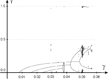
Figure 1: Bifurcation diagram, $R=0.85$, $\gamma\in[0,\ 0.06]$.

In Fig. 1 above we show the bifurcation diagram with impact times versus $\gamma$ computed for growing $\gamma$ and $R=0.85$. It follows that dynamical system (2.1), (2.2) has several attractors: two fixed points which after one period doubling give rise to chaotic bands and two other fixed points which go to chaos via period doubling scenario. There are also several small attractors. We shall investigate some of these attractors in the next Section combining analytical and numerical approach. General analytical conditions for birth of new modes of motion were given in [16].

3 Analytical and numerical results

3.1 Fixed points and their stability

We shall first study periodic solutions with one impact per $k$ periods. Such states have to fulfill the following conditions:

$$V_{n+1}=V_{n}\equiv V_{\ast}^{\left(k/1\right)},\ T_{n+1}=T_{n}+k\equiv T_{\ast}^{\left(k/1\right)}+k\qquad\left(k=1,2,\ldots\right),$$ (3.3)

where:

$$T_{\ast}^{\left(k/1\right)}\in\left(0,\ 1\right),\ V_{\ast}^{\left(k/1\right)}>\gamma\dot{Y}_{c_{1}}\left(T_{\ast}^{\left(k/1\right)}\right).$$ (3.4)

Substituting these conditions into (2.1), (2.2) we obtain two sets of fixed points:

$$0 \leq T_{\ast\left(s\right)}^{\left(k/1\right)}=\tfrac{1}{2}-\tfrac{\sqrt{3}}{18\gamma}\sqrt{9\gamma^{2}+\sqrt{3}k\gamma\tfrac{1-R}{1+R}}\leq\tfrac{1}{2}$$ (3.5)

$$V_{\ast}^{\left(k/1\right)} = k$$

where the impact occurs in time interval $T_{\ast\left(s\right)}^{\left(k/1\right)}\in\left(0,\ \frac{1}{2}\right)$ and

$$\tfrac{1}{2} \leq T_{\ast\left(u\right)}^{\left(k/1\right)}=\tfrac{1}{2}+\tfrac{\sqrt{3}}{18\gamma}\sqrt{9\gamma^{2}+\sqrt{3}k\gamma\tfrac{1-R}{1+R}}\leq 1$$ (3.6)

$$V_{\ast}^{\left(k/1\right)} = k$$

with impacts taking place in time interval $T_{\ast\left(u\right)}^{\left(k/1\right)}\in\left(\frac{1}{2},\ 1\right)$.

Solutions (3.5) fulfill physical requirements and are stable in the following interval of $\gamma$:

$$\tfrac{\sqrt{3}}{18}k\tfrac{1-R}{1+R}\leq\gamma\leq\tfrac{\sqrt{3}}{54(1+R)^{2}}\left(3k(R^{2}-1)+\sqrt{9k^{2}(R^{2}-1)^{2}+12(R^{2}+1)^{2}}\right)$$ (3.7)

where lower bound is a consequence of $T_{\ast\left(s\right)}^{\left(k/1\right)}\geq 0$ while the upper bound follows from the condition that eigenvalues $\lambda$ of the stability matrix obey $\left|\lambda\right|<1$. Accordingly, for $R=0.85$ there are only four stable fixed points with $k=1,\ 2,\ 3,\ 4$, shown in Fig. 1 – they appear at $T=0$ and $\gamma=0.0078,\ 0.0156,\ 0.0234,\ 0.0312$, respectively.

On the other hand, solutions (3.6) are always unstable and are physical for:

$$\tfrac{\sqrt{3}}{18}k\tfrac{1-R}{1+R}\leq\gamma,$$ (3.8)

what is equivalent to the condition $T_{\ast\left(u\right)}^{\left(k/1\right)}\leq 1$.

3.2 Birth of stable $2$ - cycles and transition to chaos

Let us note that $2$ - cycles are created from fixed points such that $T_{i}\in\left[0,1\right],\ T_{i+1}\in\left[k,k+1\right]$ with $k=1,2,3,4$. Therefore equations defining $2$ - cycles read:

$$\left\{\begin{array}[]{l}\gamma Y\left(\hat{T}_{i+1}\right)=\gamma Y\left(T_{i}\right)-\left(T_{i+1}-T_{i}\right)^{2}+\left(T_{i+1}-T_{i}\right)V_{i}\\ V_{i+1}=-RV_{i}+2R\left(T_{i+1}-T_{i}\right)+\gamma\left(1+R\right)\dot{Y}\left(\hat{T}_{i+1}\right)\\ \hat{T}_{i+1}\equiv T_{i+1}-k\\ \gamma Y\left(\hat{T}_{i+2}\right)=\gamma Y\left(\hat{T}_{i+1}\right)-\left(T_{i+2}-\hat{T}_{i+1}\right)^{2}+\left(T_{i+2}-\hat{T}_{i+1}\right)V_{i+1}\\ V_{i+2}=-RV_{i+1}+2R\left(T_{i+2}-\hat{T}_{i+1}\right)+\gamma\left(1+R\right)\dot{Y}\left(\hat{T}_{i+2}\right)\\ \hat{T}_{i+2}\equiv T_{i+2}-k\\ \hat{T}_{i+2}=T_{i}\\ V_{i+2}=V_{i}\end{array}\right.$$ (3.9)

where $k=1,2,3,4$ and $Y,\ \dot{Y}$ are given by (2.2). We know that $2$ - cycles appear for $\gamma=\tfrac{\sqrt{3}}{54(1+R)^{2}}\left(3k(R^{2}-1)+\sqrt{9k^{2}(R^{2}-1)^{2}+12(R^{2}+1)^{2}}\right)$, cf. Eq.(3.7). We have solved the set of equations (3.9) in closed form but we skip these lengthy formulae because of lack of space.

The bifurcation diagram shown in Fig. 1 suggests that in the case of two fixed points with $k=3,4$ transition to chaos occurs after the first period doubling when $T_{\ast 1}=0$. Therefore, in order to determine values of parameters at which the transition to chaos occurs, we have to solve Eq.(3.9) with condition $T_{i}=0$. After this substitution equations (3.9) are easily solved to yield:

$$\left\{\begin{array}[]{l}a_{4}X^{4}+a_{3}X^{3}+a_{2}X^{2}+a_{1}X+a_{0}=0\vskip 3.0pt plus 1.0pt minus 1.0pt\\ a_{4}=\left(R+1\right)^{2}\\ a_{3}=-k\left(R+1\right)\left(7R+1\right)\\ a_{2}=k\left(10k+3\right)R^{2}+\left(10R-8\right)k^{2}-3k\\ a_{1}=4k^{2}\left(\left(3-R\right)k+3\right)\\ a_{0}=-2k^{2}\left(k+1\right)\left(2k+1\right)\left(1+R^{2}\right)\vskip 3.0pt plus 1.0pt minus 1.0pt\\ \gamma_{cr}^{\left(k\right)}=\frac{\sqrt{3}X}{18\left(1+R\right)}\frac{-\left(R+1\right)^{2}X+4Rk}{\left(2+4R\right)X^{3}-3\left(R+1\right)\left(2k+1\right)X^{2}+6k\left(k+1\right)X+k\left(k+1\right)\left(2k+1\right)\left(R-1\right)}\end{array}\right.$$ (3.10)

where $X\equiv T_{i+1}$.

For example, for $R=0.85$ and $k=4$ we get from (3.10) $\gamma_{cr}^{\left(4\right)}\cong 0.03284$ while for $R=0.85$ and $k=3$ we obtain $\gamma_{cr}^{\left(3\right)}\cong 0.03806$ and indeed, precisely at this point on the $\gamma$ axis, branches of the corresponding $2$ - cycles reach values $T_{\ast 1}=0$ and transform into chaotic bands. This scenario does not apply for $R=0.85$ and $k=1,2$ - in the case $k=2$ there is another period doubling prior to $\gamma_{cr}^{\left(2\right)}$ while for $k=1$ physical solutions of (3.10) do not exist.

3.3 $N$ impacts in one period of limiter’s motion and chattering

In the bouncing ball dynamics chattering and chaotic dynamics arise typically, see [17, 18] where chattering mechanism was studied numerically for sinusoidal motion of the table. Due to simplicity of our model analytical computations are possible.

Let us assume that $N=2$ impacts, $T_{i}$, $T_{i+1}$, occur in the same period. Then the solution $\Delta_{i+1}=0$ of equation (2.1a) is always present. We thus obtain from Eqs.(2.1a) and (2.2a):

$$\Delta_{i+1} = 0,\quad\frac{1}{4G}\left(3G-2-6GT_{i}\pm\sqrt{D}\right),$$ (3.11a)

$$D = -12G^{2}T_{i}^{2}+\left(24G+12G^{2}\right)T_{i}+G^{2}-12G+16GV_{i}+4,$$ (3.11b)

where $$G\equiv 12\sqrt{3}\gamma \Delta_{i+1}\equiv T_{i+1}-T_{i}$$, . We can now rewrite Eqs.(2.1) in simplified form:

$$\left\{\begin{array}[]{l}T_{i+1}=T_{i}+\Delta_{i+1}\\ v_{i+1}=-Rv_{i}+2R\Delta_{i+1}+3RG\Delta_{i+1}\left(\Delta_{i+1}+2T_{i}-1\right)\end{array}\right.$$ (3.12c)

$$\Delta_{i+1} = \tfrac{1}{4G}\left(3G-2-6GT_{i}+\sqrt{\left(3G-2-6GT_{i}\right)^{2}+16Gv_{i}}\right)$$ (3.12d)

where $$v_{i}=V_{i}-G\left(3T_{i}^{2}-3T_{i}+\tfrac{1}{2}\right) \Delta_{i+1}>0 N\rightarrow\infty v_{\ast}=0,\ T_{i+1}=T_{i}\equiv T_{\ast} \Delta_{i+1}=0 3G-2-6GT_{\ast}\leq 0$$ is a relative velocity and the solution , cf. Eqs. (3.11), was chosen. Equations (3.12) define an explicit nonlinear map. This formalism makes possible analysis of chattering and grazing in the limit. It follows immediately that grazing manifold, , i.e. , exists only for and hence for

$$1\geq T_{\ast}\geq\max\left(T_{cr},\ 0\right),\quad T_{cr}\overset{df}{=}\tfrac{1}{2}-\tfrac{1}{3G}.$$ (3.13)

After computing eigenvalues $\Lambda_{1,2}$ of the stability matrix $S$ on the grazing manifold, $v_{\ast}=0,\ 3G-2-6GT_{\ast}\leq 0$, we get after straightforward calculations $\Lambda_{1}=1$, $\Lambda_{2}=R<1$. It thus follows that the grazing manifold is always attracting in one eigendirection and neutral in another ($T$).

In the final stage of grazing $v_{i}$ is very small. Let $3G-2-6GT_{i}<0$. It follows that for $0<x_{i}<1$, $x_{i}\overset{df}{=}\tfrac{16Gv_{i}}{\left(-3G+2+6GT_{i}\right)^{2}}$, we get the convergent expansion of the square-root in (3.12d):

$$\Delta_{i}=\tfrac{-3G+2+6GT_{i}}{4G}\left(\tfrac{1}{2}x_{i}-\tfrac{1}{8}x_{i}^{2}+\ldots\right)\cong\tfrac{2v_{i}}{-3G+2+6GT_{i}}$$ (3.14)

and the inequality $x_{i}<1$ implies:

$$T_{i}>T_{A_{1}}\equiv\left(\tfrac{1}{2}-\tfrac{1}{3G}\right)+\tfrac{2}{3}\sqrt{\tfrac{v_{i}}{G}}.$$ (3.15)

Approximate equations describing chattering, obtained from the approximate equation (3.14) and exact equations (3.12c), are of form:

$$T_{i+1} = T_{i}+\tfrac{2v_{i}}{-3G+2+6GT_{i}},$$ (3.16a)

$$v_{i+1} = \lambda_{i}v_{i},\quad\lambda_{i}\overset{df}{=}R\left(1+\tfrac{12Gv_{i}}{\left(-3G+2+6GT_{i}\right)^{2}}\right),$$ (3.16b)

and to ensure convergence $$v_{i}\rightarrow 0 \lambda_{i}<1 x_{i}<\frac{4}{3}(R^{-1}-1) T_{i}$$ we assume that (i.e. ) – this leads to the following condition for :

$$T_{i}>T_{A_{2}}\equiv\left(\tfrac{1}{2}-\tfrac{1}{3G}\right)+\sqrt{\tfrac{Rv_{i}}{3\left(1-R\right)G}}.$$ (3.17)

It is now possible to estimate time of $N$-th impact:

$$T_{\left(N\right)}\overset{df}{=}T_{i}+\sum\nolimits_{j=i+1}^{i+N}\Delta_{j}.$$ (3.18)

The time $T_{\left(N\right)}$ can be computed exactly since

$$\Delta_{j+1}=\tfrac{2v_{j}}{-3G+2+6GT_{j}}=\tfrac{2v_{j-1}\lambda_{j-1}}{-3G+2+6G\left(T_{j-1}+\Delta_{j}\right)}=\tfrac{2v_{j-1}}{-3G+2+6GT_{j-1}}R=R\Delta_{j},$$ (3.19)

where equations (3.14), (3.16b) were used, and thus

$$T_{\left(N\right)}=T_{i}+\tfrac{2v_{i}}{-3G+2+6GT_{i}}\sum\nolimits_{j=1}^{N}R^{j-1}=T_{i}+\tfrac{2v_{i}}{-3G+2+6GT_{i}}\tfrac{1-R^{N}}{1-R}.$$ (3.20)

If the ball impacts at time $T_{cr}<T_{i}<1$, performs infinite number of impacts and sticks (in one interval of limiter’s motion) then the time is $T_{\left(\infty\right)}$. Solving the inequality $T_{\left(\infty\right)}<1$ we get conditions for grazing:

$$T_{i} > T_{B}\equiv\tfrac{1}{12G}\left(\left(-2+9G\right)-\sqrt{\left(3G+2\right)^{2}-\tfrac{48Gv_{i}}{1-R}}\right)>T_{cr}\,,$$ (3.21)

$$T_{i} < T_{C}\equiv\tfrac{1}{12G}\left(\left(-2+9G\right)+\sqrt{\left(3G+2\right)^{2}-\tfrac{48Gv_{i}}{1-R}}\right)<1\,.$$ (3.22)

Finally, the (approximate) condition for grazing is: $\max\left(T_{A_{1},}T_{A_{2}},T_{B}\right)<T_{i}<T_{C}$, cf. Eqs. (3.15), ( 3.17), (3.21), (3.22).

4 Summary

It has been shown that some chaotic bands are created from fixed points after first period doubling in a corner-type bifurcation and critical values of control parameter $\gamma$ have been determined. Equations for $N$ impacts in one period of limiter’s motion were found and simplified significantly, making analysis of chattering and grazing possible. Approximate equations describing final stage of chattering were obtained and (approximate) condition for grazing was computed in analytical form.

Acknowledgement.

The paper was presented at the 11th Conference on Dynamical Systems – Theory and Applications. December 5-8, 2011. Łódź, POLAND.

References

- [1] M. di Bernardo, C.J. Budd, A.R. Champneys, P. Kowalczyk, Piecewise-Smooth Dynamical Systems. Theory and Applications. Series: Applied Mathematical Sciences, vol. 163. Springer, Berlin (2008).
- [2] A.C.J.Luo, Singularity and Dynamics on Discontinuous Vector Fields. Monograph Series on Nonlinear Science and Complexity, vol. 3. Elsevier, Amsterdam (2006).
- [3] J. Awrejcewicz, C.-H. Lamarque, Bifurcation and Chaos in Nonsmooth Mechanical Systems.World Scientific Series on Nonlinear Science: Series A, vol. 45. World Scientific Publishing, Singapore (2003).
- [4] A.F. Filippov, Differential Equations with Discontinuous Right-Hand Sides. Kluwer Academic, Dordrecht (1988).
- [5] W.J. Stronge, Impact mechanics. Cambridge University Press, Cambridge (2000).
- [6] A. Mehta (ed.), Granular Matter: An Interdisciplinary Approach. Springer, Berlin (1994).
- [7] C. Knudsen, R. Feldberg, H. True, Bifurcations and chaos in a model of a rolling wheel-set. Philos. Trans. R. Soc. Lond. A 338, 455–469 (1992).
- [8] M. Wiercigroch, A.M. Krivtsov, J. Wojewoda, Vibrational energy transfer via modulated impacts for percussive drilling, Journal of Theoretical and Applied Mechanics 46, 715–726 (2008).
- [9] A. Okniński, B. Radziszewski, Dynamics of impacts with a table moving with piecewise constant velocity, Nonlinear Dynamics 58, 515–523 (2009).
- [10] A. Okniński, B. Radziszewski, Chaotic dynamics in a simple bouncing ball model, Acta Mech. Sinica 27, 130–134 (2011), arXiv:1002.2448 [nlin.CD] (2010).
- [11] A. Okniński, B. Radziszewski, Simple model of bouncing ball dynamics: displacement of the table assumed as quadratic function of time, Nonlinear Dynamics 67, 1115—1122 (2012).
- [12] A. Okniński, B. Radziszewski, Simple models of bouncing ball dynamics and their comparison, arXiv:1002.2448 [nlin.CD] (2010).
- [13] A. Okniński, B. Radziszewski, Grazing dynamics and dependence on initial conditions in certain systems with impacts, arXiv:0706.0257 [nlin.CD] (2007).
- [14] A.C.J. Luo, R.P.S. Han, The dynamics of a bouncing ball with a sinusoidally vibrating table revisited, Nonlinear Dynamics 10, 1–18 (1996).
- [15] A. C. J. Luo, Y. Guo, Motion Switching and Chaos of a Particle in a Generalized Fermi-Acceleration Oscillator, Mathematical Problems in Engineering, vol. 2009, Article ID 298906, 40 pages, 2009. doi:10.1155/2009/298906.
- [16] A.C.J.Luo, Discontinuous Dynamical System on Time-varying Domains. Series: Nonlinear Physical Science. Higher Education Press, Beijing and Springer, Dordrecht, Heidelberg, London, New York (2009).
- [17] S. Giusepponi, F. Marchesoni, The chattering dynamics of an ideal bouncing ball, Europhysics Letters 64, 36 (2003).
- [18] S. Giusepponi, F. Marchesoni, M. Borromeo, Randomness in the bouncing ball dynamics, Physica A 351, 142–158 (2005).