A survey of lens spaces and large-scale CMB anisotropy

Abstract

The cosmic microwave background (CMB) anisotropy possesses the remarkable property that its power is strongly suppressed on large angular scales. This observational fact can naturally be explained by cosmological models with a non-trivial topology. The paper focuses on lens spaces $L(p,q)$ which are realised by a tessellation of the spherical 3-space ${\cal S}^{3}$ by cyclic deck groups of order $p\leq 72$. The investigated cosmological parameter space covers the interval $\Omega_{\hbox{\scriptsize tot}}\in[1.001,1.05]$. Several spaces are found which have CMB correlations on angular scales $\vartheta\geq 60^{\circ}$ suppressed by a factor of two compared to the simply connected ${\cal S}^{3}$ space. The analysis is based on the $S$ statistics, and a comparison to the WMAP 7yr data is carried out. Although the CMB suppression is less pronounced than in the Poincaré dodecahedral space, these lens spaces provide an alternative worth for follow-up studies.

1 Introduction

Whole sky surveys of the cosmic microwave background (CMB) sky reveal a surprisingly low power in the anisotropy at large angular scales. This property was first discovered by Hinshaw et al., (1996) using the COBE measurements and was later substantiated by the WMAP observations (Spergel et al.,, 2003). Since multiconnected spaces possess a natural lower cut-off in their wave-number spectrum $k$, they generally have less CMB anisotropy power on large scales than spaces with infinite spatial volume. Because of this property they are interesting models for the explanation of the low CMB anisotropy power.

Multiconnected spaces can be generated by tessellating the simply connected space by identifying points $u$, $u^{\prime}$ that can be mapped $u\to u^{\prime}=ug$ onto each other by applying transformations $g$ belonging to a deck group $\Gamma$. Since this paper discusses only lens spaces $L(p,q)$, the simply connected space is the spherical 3-space ${\cal S}^{3}$. The topological spaces can also be written as ${\cal M}={\cal S}^{3}/\Gamma$. An introduction to the cosmic topology is provided by Lachièze-Rey and Luminet, (1995); Luminet and Roukema, (1999); Levin, (2002); Rebouças and Gomero, (2004); Luminet, (2008). The class of lens spaces $L(p,q)={\cal S}^{3}/Z_{p}$ is specified by cyclic groups $Z_{p}$. The fundamental domains of the lens spaces can be visualised by a lens-shaped solid where the two lens surfaces are identified by a $2\pi q/p$ rotation for integers $p$ and $q$ that do not possess a common divisor greater 1 and obey $0<q<p$. Therefore, there are in general several distinct cyclic groups $Z_{p}$ which are characterised by the parameter $q$ leading to distinct spaces $L(p,q)$ having the same group order $p$ and thus the same spherical volume. For more restrictions on $p$ and $q$, see below and Gausmann et al., (2001).

In the framework of cosmic topology, the lens spaces $L(p,q)$ are first studied by Uzan et al., (2004) but the CMB properties are not studied systematically. The lens spaces $L(p,q)$ with $p\leq 500$ and $q=1$ are considered by Aurich et al., (2005), and it is found that this class does not provide models with a strong CMB suppression. The special case of group order $p=8$ is investigated by Aurich et al., (2011). The lens space sequence $q=p/2-1$ is studied by Aurich and Lustig, (2012).

The statistical CMB behaviour of the lens spaces $L(p,q)$ can be divided into two classes. The first class consists of the so-called homogeneous spaces for which the ensemble average of the CMB statistics with respect to the initial conditions is independent of the position of the CMB observer. The lens spaces $L(p,q)$ with $q=1$ belong to this class. In contrast, the inhomogeneous spaces possess ensemble averages which depend on the position of the CMB observer. These models require a much more extensive CMB analysis since it does not suffice to select a single observer position and to compute the CMB statistics for this one position. Inhomogeneous spaces must be analysed for a large distribution of different observer positions in order to decide whether they provide admissible models according to the current cosmological observations. The lens spaces $L(p,q)$ with $q>1$ are all inhomogeneous in this sense.

To elaborate this point, we have to introduce the description of the multiconnected spaces. The simply connected 3-space ${\cal S}^{3}$ is embedded in the four-dimensional Euclidean space described by the coordinates

$$\vec{x}\;=\;(x_{0},x_{1},x_{2},x_{3})^{T}\in{\cal S}^{3}$$

with the constraint $|\vec{x}\,|=1$, i. e. the 3-space ${\cal S}^{3}$ is considered as the manifold with $x_{0}^{2}+x_{1}^{2}+x_{2}^{2}+x_{3}^{2}=1$. Using complex coordinates $z_{1}:=x_{0}+\hbox{i}x_{3}$ and $z_{2}:=x_{1}+\hbox{i}x_{2}$, one can define the coordinate matrix

$$u\;:=\;\left(\begin{array}[]{cc}z_{1}&\hbox{i}z_{2}\\ \hbox{i}\overline{z}_{2}&\overline{z}_{1}\end{array}\right)\in\hbox{SU}(2,\mathbb{C})\equiv{\cal S}^{3}\hskip 10.0pt.$$ (1)

Coordinate transformations can then be described as a matrix multiplication of the coordinate matrix $u$ with a transformation matrix $t$. In the following the position of the observer is shifted by $u\to u^{\prime}=ut$ using for the transformation matrix $t$ the parameterisation

$$t(\rho,\alpha,\epsilon)\;=\;\left(\begin{array}[]{cc}\cos(\rho)\,e^{+\hbox{\scriptsize i}\alpha}&\sin(\rho)\,e^{+\hbox{\scriptsize i}\epsilon}\\ -\sin(\rho)\,e^{-\hbox{\scriptsize i}\epsilon}&\cos(\rho)\,e^{-\hbox{\scriptsize i}\alpha}\end{array}\right)$$ (2)

with $\rho\in[0,\frac{\pi}{2}]$, $\alpha,\epsilon\in[0,2\pi]$. It turns out that the CMB anisotropy depends only on the parameter $\rho$ (Aurich et al.,, 2011; Aurich and Lustig,, 2012). The independence of the CMB statistics of the parameters $\alpha$ and $\epsilon$ is the advantage of the parameterisation (2) since it allows to study the variation of the statistical properties as a one-dimensional sequence of $\rho\in[0,\frac{\pi}{2}]$. Some of the lens spaces $L(p,q)$ possess the same CMB statistics for $\rho$ and $\frac{\pi}{2}-\rho$. This allows to restrict the analysis to $\rho\in[0,\frac{\pi}{4}]$ for these spaces.

The lens spaces $L(p,q)$ and $L(p^{\prime},q^{\prime})$ are homeomorphic if and only if $p=p^{\prime}$ and either $q=\pm q^{\prime}(\hbox{mod }p)$ or $q\,q^{\prime}=\pm 1(\hbox{mod }p)$ (Gausmann et al.,, 2001). Two lens spaces $L(p,q)$ and $L(p,q^{\prime})$ with $q\,q^{\prime}=\pm 1(\hbox{mod }p)$ are usually considered as one model and only one of them is taken into account. It turns out, however, that the statistical properties of such two models are related so that the properties of the interval $\rho\in[0,\frac{\pi}{4}]$ of one model are identical to those of the interval $\rho\in[\frac{\pi}{4},\frac{\pi}{2}]$ of the other model. In the following, we thus consider two such models as distinct but analyse their CMB statistic only on the restricted interval $\rho\in[0,\frac{\pi}{4}]$. The remaining models without such a partner are exactly those with the symmetry with respect to $\rho$ and $\frac{\pi}{2}-\rho$. In this way, all possible values are computed by considering all models only for observer positions in $\rho\in[0,\frac{\pi}{4}]$.

Our simulations are based on cosmological parameters close to the concordance model. We use for the density parameter of the cold dark matter $\Omega_{\hbox{\scriptsize cdm}}=0.238$, for the density parameter of the baryonic matter $\Omega_{\hbox{\scriptsize bar}}=0.0485$, and for the Hubble constant $h=0.681$. The density parameter of the cosmological constant $\Omega_{\scriptsize\Lambda}$ is varied so that the total density parameter $\Omega_{\hbox{\scriptsize tot}}$ is in the range $\Omega_{\hbox{\scriptsize tot}}\in[1.001,1.05]$. Therefore, the models are almost flat and possess only a slight positive curvature. In addition, the spectral index $n_{\hbox{\scriptsize s}}$ is chosen to be $n_{\hbox{\scriptsize s}}=0.961$. The CMB code incorporates the full Boltzmann physics, e. g. the ordinary and the integrated Sachs-Wolfe effect, the Doppler contribution, the Silk damping and the reionisation are taken into account. The reionisation model of Aurich et al., (2008) is applied with the reionisation parameters $\alpha=0.4$ and $\beta=9.85$. The correlation function $C(\vartheta)$ and multipole moments $C_{l}$ of lens spaces are computed along the lines given by Aurich and Lustig, (2012).

2 CMB properties of lens spaces

As discussed in the Introduction, a main motivation for cosmic topology derives from the observed low power in the anisotropy at large angular scales. This suppression of CMB correlations on large angular scales is most clearly revealed by the temperature 2-point correlation function $C(\vartheta)$. It is defined as

$$C(\vartheta)\;:=\;\left<\delta T(\hat{n})\delta T(\hat{n}^{\prime})\right>\hskip 10.0pt\hbox{with}\hskip 10.0pt\hat{n}\cdot\hat{n}^{\prime}=\cos\vartheta\hskip 10.0pt,$$ (3)

where $\delta T(\hat{n})$ is the temperature fluctuation in the direction of the unit vector $\hat{n}$. The brackets $\left<\dots\right>$ denote an averaging over the directions $\hat{n}$.

The large angular behaviour is probably at variance with the $\Lambda$CDM concordance model based on a space with infinite volume as emphasised by Aurich et al., (2008); Copi et al., (2009, 2010). The correlation $C(\vartheta)$ depends on the data from which it is derived and, therefore, it is relevant which mask is applied to the WMAP data. Copi et al., (2009) infer from their investigations that only $0.025\%$ of realisations of the concordance model can describe the low correlations on separation scales greater than $60^{\circ}$ in the WMAP data admitted by the KQ75 mask. It should be noted, however, that a reconstruction algorithm can be applied to estimate the masked sky regions and it is claimed by Efstathiou et al., (2010); Bennett et al., (2011) that there is no discordance to the $\Lambda$CDM concordance model in this case. In the following, we assume that the discordance is real (Aurich and Lustig,, 2011; Copi et al.,, 2011). This section is devoted to an analysis independent of observational data. In the next section the correlations of the lens spaces $L(p,q)$ are compared to the correlations obtained from the WMAP ILC 7yr map (Gold et al.,, 2011) without a mask and with the KQ85 7yr and KQ75 7yr masks.

The suppression of CMB power becomes obvious for angular scales above $60^{\circ}$. In order to quantify this observation by a scalar measure, the $S$ statistics

$$S\;:=\;\int^{\cos(60^{\circ})}_{\cos(180^{\circ})}d\cos\vartheta\;|C(\vartheta)|^{2}$$ (4)

has been introduced by Spergel et al., (2003). Although this statistics eliminates the information about the correlation function $C(\vartheta)$, it has the advantage that different simulations of $L(p,q)$ can be compared by a single number.

For all lens spaces $L(p,q)$ with $p\leq 72$, the correlation function $C(\vartheta)$ is computed on a two-dimensional grid with the axes $\rho\in[0,\frac{\pi}{4}]$ and $\Omega_{\hbox{\scriptsize tot}}\in[1.001,1.05]$. The $\rho$ interval is discretised by 101 equidistant points. For the $\Omega_{\hbox{\scriptsize tot}}$ interval, the step width $\Delta\Omega_{\hbox{\scriptsize tot}}=0.001$ is used on $[1.001,1.03]$ and $\Delta\Omega_{\hbox{\scriptsize tot}}=0.002$ on $[1.03,1.05]$. It would be desirable to use an even finer grid close to the $\Omega_{\hbox{\scriptsize tot}}=1.001$ border, but this is numerically too demanding. The mesh consists of 4040 grid points at which $C(\vartheta)$ is to be computed for each lens space leading to a total of 2,923,760 simulations that are to be analysed. From this grid, the best value for $S_{L(p,q)}(\Omega_{\hbox{\scriptsize tot}},\rho)$ is selected, which is the smallest one in order to get the maximal suppression in CMB power on angular scales with $\vartheta\geq 60^{\circ}$. We would like to note that the range $\Omega_{\hbox{\scriptsize tot}}\in[1,1.001]$ is not covered by our survey so that there is the possibility that some models selected at the border $\Omega_{\hbox{\scriptsize tot}}=1.001$ might be even better if smaller values of $\Omega_{\hbox{\scriptsize tot}}$ would be accessible. It turns out that there are indeed models having their minimum at $\Omega_{\hbox{\scriptsize tot}}=1.001$. Such an example is given by the homogeneous lens spaces $L(p,1)$ where the minimum is at $\Omega_{\hbox{\scriptsize tot}}=1.001$ for $p\gtrsim 40$.

Figure 1: The difference in the normalisations of eqs. (5) and (6) is shown by plotting the ratio $S_{{\cal S}^{3}}(\Omega_{\hbox{\scriptsize tot}})/S_{{\cal S}^{3}}(\Omega_{\hbox{\scriptsize tot}}=1.001)$.

Before the minimum is searched, the $S_{L(p,q)}(\Omega_{\hbox{\scriptsize tot}},\rho)$ statistics is normalised in two different ways to the $S_{{\cal S}^{3}}(\Omega_{\hbox{\scriptsize tot}})$ statistics of the simply connected 3-space ${\cal S}^{3}$. In the first procedure, $S_{L(p,q)}(\Omega_{\hbox{\scriptsize tot}},\rho)$ is normalised to the value of $S_{{\cal S}^{3}}(\Omega_{\hbox{\scriptsize tot}})$ with the same $\Omega_{\hbox{\scriptsize tot}}$, and then, the minimum is looked for

$$S_{\Omega}\;:=\;\min_{\Omega_{\hbox{\scriptsize tot}},\rho}\;\frac{S_{L(p,q)}(\Omega_{\hbox{\scriptsize tot}},\rho)}{S_{{\cal S}^{3}}(\Omega_{\hbox{\scriptsize tot}})}\hskip 10.0pt.$$ (5)

In the second procedure, $S_{L(p,q)}(\Omega_{\hbox{\scriptsize tot}},\rho)$ is normalised to the value of $S_{{\cal S}^{3}}(\Omega_{\hbox{\scriptsize tot}})$ taken at $\Omega_{\hbox{\scriptsize tot}}=1.001$ leading to

$$S_{\Lambda}\;:=\;\min_{\Omega_{\hbox{\scriptsize tot}},\rho}\;\frac{S_{L(p,q)}(\Omega_{\hbox{\scriptsize tot}},\rho)}{S_{{\cal S}^{3}}(\Omega_{\hbox{\scriptsize tot}}=1.001)}\hskip 10.0pt.$$ (6)

The first normalisation $S_{\Omega}$ emphasises the topological aspect since it compares the multiconnected space with the simply connected spherical 3-space ${\cal S}^{3}$ at the same value of $\Omega_{\hbox{\scriptsize tot}}$. The second normalisation $S_{\Lambda}$ can be considered as a comparison with the $\Lambda$CDM concordance model since $\Omega_{\hbox{\scriptsize tot}}=1.001$ is nearly indistinguishable from the flat case. The figure 1 displays the ratio $S_{{\cal S}^{3}}(\Omega_{\hbox{\scriptsize tot}})/S_{{\cal S}^{3}}(\Omega_{\hbox{\scriptsize tot}}=1.001)$ in order to allow a comparison between the two statistics defined in eqs. (5) and (6).

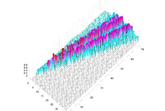
Figure 2: The minimum of the $S_{\Omega}$ statistics for the lens spaces $L(p,q)$ is extracted from the grid with axes $\rho\in[0,\frac{\pi}{4}]$ and $\Omega_{\hbox{\scriptsize tot}}\in[1.001,1.05]$. To emphasise small values of $S_{\Omega}$, the height of the bins is proportional to $1/S_{\Omega}-1$, i. e. larger bins correspond to smaller CMB power. Therefore, a value of zero indicates that the suppression of the CMB power is the same as for the simply connected ${\cal S}^{3}$ space. Note, that the $S_{\Omega}$ statistics is normalised to that of the simply connected 3-space ${\cal S}^{3}$ with the same $\Omega_{\hbox{\scriptsize tot}}$.

Figure 2 provides an overview of the lens spaces $L(p,q)$ parameterised by the group order $p$ and $q$ together with their CMB suppression of correlations on large angles. In order to emphasise the positions $(p,q)$ with small values of $S_{\Omega}$, the height of the bins is chosen as $1/S_{\Omega}-1$. Here, the value of $S_{\Omega}$ is the minimum found in the parameter range $\rho\in[0,\frac{\pi}{4}]$ and $\Omega_{\hbox{\scriptsize tot}}\in[1.001,1.05]$ for a given lens space $L(p,q)$. The figure reveals that, for fixed $p$, medium values of $q$ provide in many cases models with a stronger CMB suppression than values close to $q=1$ or to the maximal possible $q=p/2-1$. Since the angle $2\pi q/p$ is the angle by which the two surfaces of a lens have to be rotated relatively to each other before they are identified, the best CMB suppression is found for medium rotation angles. The best candidate lens spaces concentrate along the two lines with $q\simeq 0.28p$ and $q\simeq 0.38p$. This corresponds to rotation angles of $101^{\circ}$ and $137^{\circ}$ independent of the group order $p$.

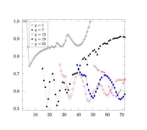
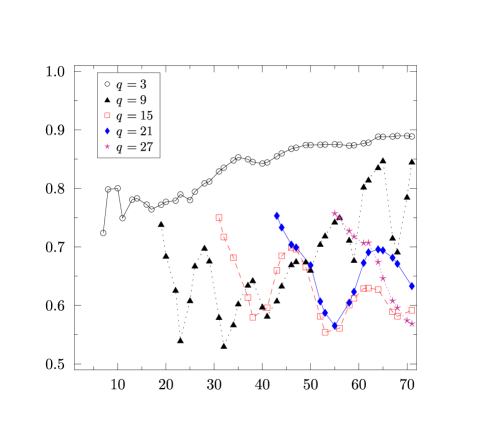
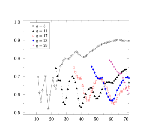
Figure 3: The $S_{\Omega}$ statistics is plotted for odd values of $q$ as a function of the group order $p$.

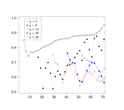
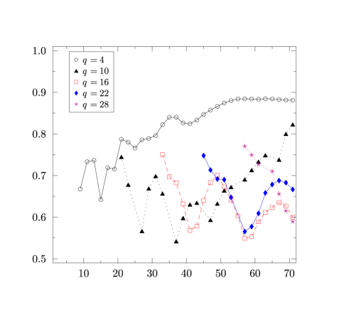
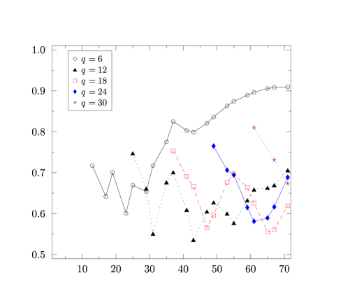
Figure 4: The $S_{\Omega}$ statistics is plotted for even values of $q$ as a function of the group order $p$.

The figure 2 is too complex in order to reveal the lens spaces $L(p,q)$ with the strongest CMB suppression. For that reason, the figures 3 and 4 show cross-sections of figure 2 so that the $S_{\Omega}$ dependence on the group order $p$ can be inferred. Small values of $S_{\Omega}$ are favoured by the observations. The $S_{\Omega}$ statistics is shown for various values of $q$. Figures 3 and 4 show odd and even values of $q$, respectively. The values of $q$ are distributed over the three panels in such a way that their curves do not entangle too much. There are several models $L(p,q)$ for which the CMB suppression is almost twice that of the simply connected spherical 3-space ${\cal S}^{3}$. The inspection of figure 3 reveals several $q$-curves with a significant CMB power suppression on large angular scales. For example, the $q=9$ curve possesses two pronounced minima at $p=23$ and $p=32$. These two minima belong to the two diagonals $q\simeq 0.28p$ and $q\simeq 0.38p$ mentioned in the discussion of figure 2. The anisotropy measured by $S_{\Omega}$ is almost a factor 2 smaller than for the simply connected ${\cal S}^{3}$. However, one does not find a single lens space or at least a few candidates with a significant CMB suppression, but instead there are many lens spaces as received from the figures 3 and 4. A lot of models have values of $S_{\Omega}$ between 0.5 and 0.6. The table 1 lists the 10 lens spaces with the strongest CMB anisotropy suppression that are found on our $\Omega_{\hbox{\scriptsize tot}}$-$\rho$ grid. The $L(32,9)$ lens space belonging to the $q=9$ curve is found at the sixth place in table 1. In addition, the table also gives the value of $\Omega_{\hbox{\scriptsize tot}}$ and the observer position parameterised by $\rho$ where the minimum is found.

The homogeneous lens spaces $L(p,1)$ do not possess a pronounced suppression of CMB power as revealed by the first panel of figure 3. Since the deck group consists only of Clifford translations for $q=1$, the fundamental domain ${\cal F}$ defined as a Voronoi domain is independent of the observer position and so are the CMB properties (Aurich et al.,, 2011; Aurich and Lustig,, 2012). This is in contrast to the models with $q>1$ which are all inhomogeneous. The absence of such a variability disfavours the homogeneous lens spaces $L(p,1)$.

Up to now, the $S_{\Omega}$ statistics defined in eq. (5) is used which emphasises the topological aspect. The table 2 gives the ten best lens spaces $L(p,q)$ found on our grid, when the definition (6) is used. A comparison with table 1 lead to the conclusion that the application of the $S_{\Lambda}$ statistics favours lens spaces $L(p,q)$ with a larger group order $p$ and a smaller value of $\Omega_{\hbox{\scriptsize tot}}$. This is caused by the fact that the $S_{\Lambda}$ statistics compares the CMB correlations with that of the almost flat $\Lambda$CDM concordance model with $\Omega_{\hbox{\scriptsize tot}}=1.001$. This in turn favours models that are as flat as possible leading to a focus on spaces with a large group order $p$.

Table 1: The lens spaces $L(p,q)$ with the largest suppression measured by $S_{\Omega}$ are listed together with the position in our $\Omega_{\hbox{\scriptsize tot}}$-$\rho$ grid.

${\cal M}$	$S_{\Omega}$	$\Omega_{\hbox{\scriptsize tot}}$	$\rho$
$L(18,7)$	0.51260	1.044	0.43 $\pi/4$
$L(25,7)$	0.51954	1.034	0.48 $\pi/4$
$L(18,5)$	0.52109	1.050	0.58 $\pi/4$
$L(29,8)$	0.52235	1.027	0.43 $\pi/4$
$L(21,8)$	0.52481	1.034	0.37 $\pi/4$
$L(32,9)$	0.53090	1.023	0.39 $\pi/4$
$L(40,11)$	0.53111	1.016	0.33 $\pi/4$
$L(43,12)$	0.53594	1.014	0.31 $\pi/4$
$L(39,11)$	0.53915	1.016	0.32 $\pi/4$
$L(47,13)$	0.53946	1.011	0.27 $\pi/4$

Table 2: The lens spaces $L(p,q)$ with the largest suppression measured by $S_{\Lambda}$ are listed together with the position in our $\Omega_{\hbox{\scriptsize tot}}$-$\rho$ grid.

${\cal M}$	$S_{\Lambda}$	$\Omega_{\hbox{\scriptsize tot}}$	$\rho$
$L(71,27)$	0.59506	1.003	0.09 $\pi/4$
$L(69,19)$	0.59575	1.005	0.17 $\pi/4$
$L(70,19)$	0.59836	1.005	0.17 $\pi/4$
$L(62,17)$	0.59970	1.007	0.22 $\pi/4$
$L(65,18)$	0.60023	1.006	0.20 $\pi/4$
$L(51,14)$	0.60026	1.009	0.24 $\pi/4$
$L(69,26)$	0.60055	1.003	0.09 $\pi/4$
$L(68,19)$	0.60073	1.006	0.20 $\pi/4$
$L(61,17)$	0.60079	1.007	0.22 $\pi/4$
$L(70,27)$	0.60082	1.003	0.09 $\pi/4$

3 Comparison with the WMAP data

The $S$ statistics analysed in the previous section has the great advantage that it measures large scale correlations independent of observational data. The $S$ statistics allows to find topological spaces with a CMB suppression on large angular scales. In this section, the correlation function $C(\vartheta)$ is compared with the correlation function obtained from the WMAP 7yr data (Gold et al.,, 2011). In order to compare the correlation function $C^{\hbox{\scriptsize model}}(\vartheta)$ with the observed correlation function $C^{\hbox{\scriptsize obs}}(\vartheta)$, the integrated weighted temperature correlation difference is introduced by Aurich et al., (2008)

$$I:=\int_{-1}^{1}d\cos\vartheta\;\;\frac{(C^{\hbox{\scriptsize model}}(\vartheta)-C^{\hbox{\scriptsize obs}}(\vartheta))^{2}}{\hbox{Var}(C^{\hbox{\scriptsize model}}(\vartheta))}$$ (7)

which tests all angular scales $\vartheta\in[0^{\circ},180^{\circ}]$. This is in contrast to the $S$ statistics which focuses on the large angular range $\vartheta\geq 60^{\circ}$. The variance is calculated by using

$$\hbox{Var}(C(\vartheta))\;\approx\;\sum_{l}\frac{2l+1}{8\pi^{2}}\,\left[C_{l}\,P_{l}(\cos\vartheta)\right]^{2}\hskip 10.0pt.$$ (8)

The correlation function $C^{\hbox{\scriptsize model}}(\vartheta)$ is the ensemble average with respect to the Gaussian initial conditions. However, the ensemble average depends on the observer position.

The integrated weighted temperature correlation difference $I$ is computed on the $\Omega_{\hbox{\scriptsize tot}}$-$\rho$ grid and the minimum $I_{\hbox{\scriptsize min}}$ is determined in order to find the best simulation for each lens space. Now one has to specify the observational data on which $C^{\hbox{\scriptsize obs}}(\vartheta)$ is based. As discussed at the beginning of section 2, the correlation function $C^{\hbox{\scriptsize obs}}(\vartheta)$ depends significantly on the chosen mask that is applied to the WMAP ILC map. For that reason we compute $C^{\hbox{\scriptsize obs}}(\vartheta)$ for three cases. In the first case $C^{\hbox{\scriptsize obs}}(\vartheta)$ is computed from the whole WMAP ILC 7yr map that is without applying a mask. In the other two cases the two masks KQ85 7yr and KQ75 7yr are applied which are provided by Gold et al., (2011). The masks include 78.3% and 70.6% of the sky for the KQ85 7yr and KQ75 7yr masks, respectively.

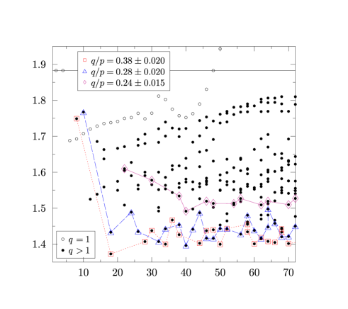
Figure 5: The minima $I_{\hbox{\scriptsize min}}$ of the $I$ statistics are plotted as a function of the group order $p$ for each lens space $L(p,q)$. $C^{\hbox{\scriptsize obs}}(\vartheta)$ is obtained from the full WMAP ILC 7yr map. The homogeneous lens spaces $L(p,1)$ are shown as circles, and the inhomogeneous ones as full discs. In addition, the three sequences with $q/p=0.38$, $q/p=0.28$, and $q/p=0.24$ are marked as squares, triangles, and diamonds, respectively. The panel (a) shows only lens spaces with an odd group order $p$, and panel (b) only those with an even group order $p$.

The minima $I_{\hbox{\scriptsize min}}$ of the $I$ statistics computed from these three correlation functions $C^{\hbox{\scriptsize obs}}(\vartheta)$ are presented in figures 5, 6, and 7, where the data are displayed for all lens spaces $L(p,q)$ up to group order $p=72$. The values of $I_{\hbox{\scriptsize min}}$ have to be compared with the value of the trivial topology, i. e. with the simply connected 3-space ${\cal S}^{3}\equiv L(1,1)$. The corresponding value can be read off from the case $p=1$ and is shown as the straight horizontal line. All data points which are below that of ${\cal S}^{3}\equiv L(1,1)$ describe the observed correlations better than the simply connected ${\cal S}^{3}$. All considered inhomogeneous lens spaces $(p\leq 72)$ are thus preferred to the 3-space ${\cal S}^{3}$. In section 2 we found two sequences of lens spaces $L(p,q)$ with a superior suppression of large angle correlations. These two sequences with $q\simeq 0.38p$ and $q\simeq 0.28p$ are explicitly marked in figures 5, 6, and 7. It is seen that they also attract attention in the case of the $I$ statistics. In addition to these two sequences, the figures also mark the sequence with $q\simeq 0.24p$, which leads for large group orders $p$ to interesting models, if the KQ75 mask is applied.

The figures 5, 6, and 7 reveal a remarkable behaviour. Using no mask at all one observes in figure 5 that the best models are around $p=20$ with $I_{\hbox{\scriptsize min}}$ below 1.4. This contrasts to the case with the largest mask, i. e. the KQ75 7yr mask with 70.6% sky coverage, where the smallest values of $I_{\hbox{\scriptsize min}}$ occur at much larger group orders above $p=50$, see figure 7. Surprisingly, the slightly smaller KQ85 7yr mask with 78.3% sky coverage is more similar to the case without a mask, since the smallest values of $I_{\hbox{\scriptsize min}}$ are now at low group orders. Because of the severe dependence on the chosen mask, one can only conclude that the inhomogeneous lens spaces $L(p,q)$ describe the WMAP data better than the 3-space ${\cal S}^{3}$. But the data cannot be used to single out one or at least a few lens spaces $L(p,q)$ as best candidates.

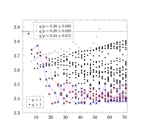
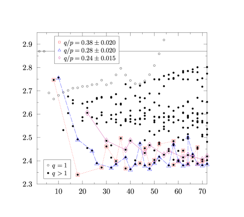
Figure 6: The minima $I_{\hbox{\scriptsize min}}$ of the $I$ statistics are shown as in figure 5. However, $C^{\hbox{\scriptsize obs}}(\vartheta)$ is obtained from the WMAP ILC 7yr map by applying the KQ85 mask.

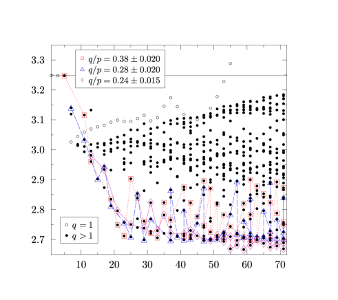
Figure 7: The minima $I_{\hbox{\scriptsize min}}$ of the $I$ statistics are shown as in figure 5. However, $C^{\hbox{\scriptsize obs}}(\vartheta)$ is obtained from the WMAP ILC 7yr map by applying the KQ75 mask.

4 Summary

In this paper a class of topological spaces based on cyclic groups $Z_{p}$ is investigated with respect to their CMB properties. These spaces are the lens spaces $L(p,q)$ of group order $p\leq 72$ which are realised in spherical spaces, i. e. with a positive spatial curvature. Only almost flat cosmological models are considered which belong to the interval $\Omega_{\hbox{\scriptsize tot}}=[1.001,1.05]$. Since the lens spaces $L(p,q)$ with $q>1$ are inhomogeneous in the sense that the ensemble average of the CMB fluctuations is dependent on the position of the observer, a careful survey is required for each inhomogeneous lens space which takes this additional complication into account. For each space $L(p,q)$ with $p\leq 72$, the CMB correlations are computed for the above range of $\Omega_{\hbox{\scriptsize tot}}$ and for a dense set of observer positions that exhausts the spatial CMB variability. From this set of almost 3 million simulations, the models with the lowest CMB correlations on large angular scales yield the interesting candidates.

The lens spaces $L(p,q)$ with $0<q<p$ are distributed in the $p$-$q$ plane within a triangular domain bounded by $q=1$, i. e. the homogeneous spaces, and $q=p/2-1$. It turns out that models with a large CMB suppression on angular scales $\vartheta\geq 60^{\circ}$ concentrate on two bands which are approximately defined by $q\simeq 0.28p$ and $q\simeq 0.38p$. There are models within these two bands which have a CMB suppression for $\vartheta\geq 60^{\circ}$ being two times stronger than the simply connected spherical 3-space ${\cal S}^{3}$.

The correlations of the lens spaces $L(p,q)$ are compared with the WMAP 7yr data using the integrated weighted temperature correlation difference (7). Three correlation functions $C(\vartheta)$ are derived from the WMAP ILC 7yr map, based on the whole map and based on the data after applying the KQ85 7yr and KQ75 7yr masks. A number of lens spaces $L(p,q)$ are found which describe the three correlation functions $C(\vartheta)$ based on the WMAP data better than the 3-space ${\cal S}^{3}$. However, it turns out that for each of the three cases other best candidates are found. Because of the sensitivity on the admitted WMAP data, no firm conclusion can be drawn and no best candidate can be selected.

We thus conclude that there are lens spaces $L(p,q)$ with $q\simeq 0.28p$ and $q\simeq 0.38p$ which display a stronger CMB suppression on large angular scales than the simply connected space. Although the CMB suppression is less pronounced than in the Poincaré dodecahedral space, where the CMB correlation for $\vartheta\geq 60^{\circ}$ is reduced by a factor 0.11 at $\Omega_{\hbox{\scriptsize tot}}=1.02$, these lens spaces provide an alternative worth for follow-up studies.

References

- Aurich et al., (2008) Aurich, R., Janzer, H. S., Lustig, S., and Steiner, F. (2008). Do we Live in a ”Small Universe”? Class. Quantum Grav., 25:125006.
- Aurich et al., (2011) Aurich, R., Kramer, P., and Lustig, S. (2011). CMB radiation in an inhomogeneous spherical space. Physica Scripta, 84:055901.
- Aurich and Lustig, (2011) Aurich, R. and Lustig, S. (2011). Can one reconstruct the masked CMB sky? Mon. Not. R. Astron. Soc., 411:124–136.
- Aurich and Lustig, (2012) Aurich, R. and Lustig, S. (2012). How well-proportioned are lens and prism spaces? arXiv:1201.6490 [astro-ph.CO].
- Aurich et al., (2005) Aurich, R., Lustig, S., and Steiner, F. (2005). CMB anisotropy of spherical spaces. Class. Quantum Grav., 22:3443–3459.
- Bennett et al., (2011) Bennett, C. L., Hill, R. S., Hinshaw, G., Larson, D., Smith, K. M., Dunkley, J., Gold, B., Halpern, M., Jarosik, N., Kogut, A., Komatsu, E., Limon, M., Meyer, S. S., Nolta, M. R., Odegard, N., Page, L., Spergel, D. N., Tucker, G. S., Weiland, J. L., Wollack, E., and Wright, E. L. (2011). Seven-Year Wilkinson Microwave Anisotropy Probe (WMAP) Observations: Are There Cosmic Microwave Background Anomalies? Astrophys. J. Supp., 192:17.
- Copi et al., (2009) Copi, C. J., Huterer, D., Schwarz, D. J., and Starkman, G. D. (2009). No large-angle correlations on the non-Galactic microwave sky. Mon. Not. R. Astron. Soc., 399:295–303.
- Copi et al., (2010) Copi, C. J., Huterer, D., Schwarz, D. J., and Starkman, G. D. (2010). Large angle anomalies in the CMB. Adv. Astron., 2010:847541.
- Copi et al., (2011) Copi, C. J., Huterer, D., Schwarz, D. J., and Starkman, G. D. (2011). Bias in low-multipole CMB reconstructions. Mon. Not. R. Astron. Soc., 418:505–515.
- Efstathiou et al., (2010) Efstathiou, G., Ma, Y.-Z., and Hanson, D. (2010). Large-Angle Correlations in the Cosmic Microwave Background. Mon. Not. R. Astron. Soc., 407:2530–2542.
- Gausmann et al., (2001) Gausmann, E., Lehoucq, R., Luminet, J.-P., Uzan, J.-P., and Weeks, J. (2001). Topological lensing in spherical spaces. Class. Quantum Grav., 18:5155–5186.
- Gold et al., (2011) Gold, B., Odegard, N., Weiland, J. L., Hill, R. S., Kogut, A., Bennett, C. L., Hinshaw, G., Chen, X., Dunkley, J., Halpern, M., Jarosik, N., Komatsu, E., Larson, D., Limon, M., Meyer, S. S., Nolta, M. R., Page, L., Smith, K. M., Spergel, D. N., Tucker, G. S., Wollack, E., and Wright, E. L. (2011). Seven-Year Wilkinson Microwave Anisotropy Probe (WMAP) Observations: Galactic Foreground Emission. Astrophys. J. Supp., 192:15.
- Górski et al., (2005) Górski, K. M., Hivon, E., Banday, A. J., Wandelt, B. D., Hansen, F. K., Reinecke, M., and Bartelmann, M. (2005). HEALPix: A Framework for High-Resolution Discretization and Fast Analysis of Data Distributed on the Sphere. Astrophys. J., 622:759–771. HEALPix web-site: http://healpix.jpl.nasa.gov/.
- Hinshaw et al., (1996) Hinshaw, G., Banday, A. J., Bennett, C. L., Górski, K. M., Kogut, A., Lineweaver, C. H., Smoot, G. F., and Wright, E. L. (1996). Two-Point Correlations in the COBE DMR Four-Year Anisotropy Maps. Astrophys. J. Lett., 464:L25–L28.
- Lachièze-Rey and Luminet, (1995) Lachièze-Rey, M. and Luminet, J.-P. (1995). Cosmic topology. Physics Report, 254:135–214.
- Levin, (2002) Levin, J. (2002). Topology and the cosmic microwave background. Physics Report, 365:251–333.
- Luminet, (2008) Luminet, J.-P. (2008). The Shape and Topology of the Universe. arXiv:0802.2236 [astro-ph].
- Luminet and Roukema, (1999) Luminet, J.-P. and Roukema, B. F. (1999). Topology of the Universe: Theory and Observation. In NATO ASIC Proc. 541: Theoretical and Observational Cosmology, page 117.
- Rebouças and Gomero, (2004) Rebouças, M. J. and Gomero, G. I. (2004). Cosmic Topology: a Brief Overview. Braz. J. Phys., 34:1358–1366.
- Spergel et al., (2003) Spergel, D. N., Verde, L., Peiris, H. V., Komatsu, E., Nolta, M. R., Bennett, C. L., Halpern, M., Hinshaw, G., Jarosik, N., Kogut, A., Limon, M., Meyer, S. S., Page, L., Tucker, G. S., Weiland, J. L., Wollack, E., and Wright, E. L. (2003). First-Year Wilkinson Microwave Anisotropy Probe (WMAP) Observations: Determination of Cosmological Parameters. Astrophys. J. Supp., 148:175–194.
- Uzan et al., (2004) Uzan, J.-P., Riazuelo, A., Lehoucq, R., and Weeks, J. (2004). Cosmic microwave background constraints on lens spaces. Phys. Rev. D, 69:043003–1–4.