SubHaloes going Notts: The SubHalo-Finder Comparison Project

Abstract

We present a detailed comparison of the substructure properties of a single Milky Way sized dark matter halo from the Aquarius suite (Springel et al.) at five different resolutions, as identified by a variety of different (sub-)halo finders for simulations of cosmic structure formation. These finders span a wide range of techniques and methodologies to extract and quantify substructures within a larger non-homogeneous background density (e.g. a host halo). This includes real-space, phase-space, velocity-space and time-space based finders, as well as finders employing a Voronoi tessellation, friends-of-friends techniques, or refined meshes as the starting point for locating substructure. A common post-processing pipeline was used to uniformly analyse the particle lists provided by each finder. We extract quantitative and comparable measures for the subhaloes, primarily focusing on mass and the peak of the rotation curve for this particular study. We find that all of the finders agree extremely well on the presence and location of substructure and even for properties relating to the inner part part of the subhalo (e.g. the maximum value of the rotation curve). For properties that rely on particles near the outer edge of the subhalo the agreement is at around the 20 per cent level. We find that basic properties (mass, maximum circular velocity) of a subhalo can be reliably recovered if the subhalo contains more than 100 particles although its presence can be reliably inferred for a lower particle number limit of 20. We finally note that the logarithmic slope of the subhalo cumulative number count is remarkably consistent and $<1$ for all the finders that reached high resolution. If correct, this would indicate that the larger and more massive, respectively, substructures are the most dynamically interesting and that higher levels of the (sub-)subhalo hierarchy become progressively less important.

1 Introduction

The growth of structure via a hierarchical series of mergers is now a well established paradigm (White & Rees, 1978). As larger structures grow they subsume small infalling objects. However the memory of the existence of these substructures is not immediately erased, either in the observable Universe (where thousands of individual galaxies within a galaxy cluster are obvious markers of this pre-existing structure) or within numerical models, first noted for the latter by Klypin et al. (1999).

Knowing the properties of substructure created in cosmological $N$-body simulations allows the most direct comparison between these simulations and observations of the Universe. The fraction of material that remains undispersed and so survives as separate structures within larger haloes is an important quantity for both studies of dark-matter detection (Springel et al., 2008; Kuhlen et al., 2008; Vogelsberger et al., 2009; Zavala et al., 2010) and the apparent overabundance of substructure within numerical models when compared to observations (Klypin et al., 1999; Moore et al., 1999). The mass and radial position of the most massive Milky Way satellites seem to raise new concerns for our standard $\Lambda$CDM cosmology (Boylan-Kolchin et al., 2011b, a; di Cintio et al., 2011; Ferrero et al., 2011), while differences between the simulated and observed internal density profiles of the satellites seems to have been reconciled by taking baryonic effects into account (e.g. Oh et al., 2011; Pontzen & Governato, 2011). We are certain that between 5 per cent and 10 per cent of the material within simulated galactic sized haloes exists within bound substructures (e.g. Gao et al., 2004; De Lucia et al., 2004; Contini et al., 2011) and a substantial part of the host halo has formed from disrupted subhalo material (e.g. Gill et al., 2004; Knebe et al., 2005; Warnick et al., 2008; Cooper et al., 2010; Libeskind et al., 2011).

Quantification of the amount of substructure (both observationally and in simulations of structure formation) is therefore an essential tool to what is nowadays referred to as “Near-Field Cosmology” (Freeman & Bland-Hawthorn, 2002) and attempts to do so in numerical models have followed two broad approaches: either a small number of individual haloes are simulated at exquisite resolution (e.g. Diemand et al., 2008; Springel et al., 2008; Stadel et al., 2009, respectively the Via Lactea, Aquarius and GHalo projects) or a larger representative sample of the Universe is modelled in order to quantify halo-to-halo substructure variations (e.g. Angulo et al., 2009; Boylan-Kolchin et al., 2009; Klypin et al., 2011, who used the Millennium simulation, Millennium II simulation and the Bolshoi simulation, respectively). As this paper studies the convergence of halo-finders within a single halo we can add nothing to the topic of halo-to-halo substructure variations.

In a very comprehensive study that included 6 different haloes and 5 levels of resolution Springel et al. (2008) utilised their substructure finder subfind to detect around 300000 substructures within the virial radius of their best resolved halo. They found that the number counts of substructures per logarithmic decade in mass falls with a power law index of at most 0.93, indicating that smaller substructures are progressively less dynamically important and that the central regions of the host dark matter halo are likely to be dominated by a diffuse dark matter component composed of hundreds of thousands of streams of tidally stripped material. Maciejewski et al. (2011) confirmed the existence and properties of this stripped material using a 6-dimensional phase-space finder hsf. A similar power law index was also found for the larger cosmological studies (Boylan-Kolchin et al., 2009; Angulo et al., 2009). For the Bolshoi simulation Klypin et al. (2011) find results that are in agreement with their re-analysis of the Via Lactea II of Diemand et al. (2008) with an abundance of subhaloes falling as the cube of the subhalo rotation velocity. Rather than the present value of the maximum rotation velocity they prefer to use the value that the subhalo had when it first became a subhalo (i.e. on infall). This negates the effects of tidal stripping and harassment within the cluster environment but makes it difficult for us to directly compare as we have generally only used the final $z=0$ snapshot for this comparison study.

In recent years there has not only been a number of different groups performing billion particle single-halo calculations, there has also been an explosion in the number of methods available for quantifying the size and location of the structures within such an $N$-body simulation (see, for instance, Fig.1 in Knebe et al., 2011). In this paper we extend the halo finder comparison study of Knebe et al. (2011) to examine how well these finders extract the properties of those haloes that survive the merging process and live within larger haloes. While this issue has already been addressed by Knebe et al. (2011) it was nevertheless only in an academic way where controlled set-ups of individual subhaloes placed into generic host haloes were studied; here we apply the comparison to a fully self-consistently formed dark matter halo extracted from a cosmological simulation. As the results of credible and reliable subhalo identification have such important implications across a wide range of astrophysics it is essential to ask how well the (sub-)halo finders perform at reliably extracting subhaloes. This still leaves open the question of how well different modern gravity solvers compare when performing the same simulation but at least we can hope to ascertain whether or not – given the same set of simulation data – the different finders will arrive at the same conclusions about the enclosed subhalo properties. We intend this paper to form the first part of a series of comparisons. It primarily focuses on the most relevant subhalo properties, i.e. location, mass spectrum and the distribution of the value of the peak of the subhaloes’ rotation curve.

In Section 2 we begin by summarising the eleven substructure finders that have participated in this study, focusing upon any elements that are of particular relevance for substructure finding. In Section 3 we introduce the Aquarius dataset that the described finders analysed for this study. Both a qualitative and a quantitative comparison between the finders is contained in Section 4 which also contains a discussion of our results, before we summarise and conclude in Section 5.

Figure 1: The images show the smoothed dark matter density within an quadrant at resolution level 4. In each panel the overplotted circles indicate the location of the recovered subhaloes for the finder labelled at the top of each panel. They are scaled proportionally using $v_{\rm max}$. Only subhaloes with a $v_{\rm max}$ greater than 10 km/s are shown.

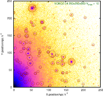
Figure 1: (continued) Recovered subhalo locations and $v_{\rm max}$ scale by labelled finder.

2 The SubHalo Finders

In this section we present the (sub-)halo finders participating in the comparison project in alphabetical order. Please note that we primarily only provide references to the actual code description papers and not an exhaustive portrait of each finder as this would be far beyond the scope of this paper. While the general mode of operation can be found elsewhere, we nevertheless focus here on the way each code collects and defines the set of particles belonging to a subhalo: as already mentioned before, those particle lists are subjected to a common post-processing pipeline and hence the retrieval of this list is the only relevant piece of information as far as the comparison in this particular paper is concerned.

2.1 ADAPTAHOP (Tweed)

adaptahop is a full topological algorithm. The first stage consist in estimating a local density using a 20 particles SPH kernel. Particles are then sorted into groups around a local density maximum. And saddle points act as links between group. All groups are first supposed to be one single entity, that we hierarchically divide into smaller groups, by using an increasing density threshold. Haloes are then defined as groups of groups linked by saddle points corresponding to densities higher that 80 times the mean DM density. By increasing the threshold we further detail the structure of the halo as a node structure tree. Where a node is either a local maxima, or a group of particules connecting higher level nodes. After using this bottom to top approach, the (sub)haloes are defined using a top to bottom approach, hierarchically regrouping nodes so that a sub(sub)halo has a smaller mass than its host (sub)halo. Each particle belongs to a single structure either a halo or a subhalo. The (sub)haloes’ centers are defined as the position of its particles with the highest SPH density. We need to stress that no unbinding procedures are used in this algorithm, at the risk of overestimating the number/misidentification of subhaloes with a low number of particles.

2.2 AHF (Knollmann & Knebe)

The halo finder ahf (amiga Halo Finder) is a spherical overdensity finder that identifies (isolated and sub-)haloes as described in Gill et al. (2004) as well as Knollmann & Knebe (2009). The initial particle lists are obtained by a rather elaborate scheme: for each subhalo the distance to its nearest more massive (sub-)halo is calculated and all particles within a sphere of radius half this distance are considered prospective subhalo constituents. This list is then pruned by an iterative unbinding procedure using the (fixed) subhalo centre as given by the local density peak determined from an adaptive mesh refinement hierarchy. For more details we refer the reader to aforementioned code description papers as well as the online documentation.

2.3 Hierarchical Bound-Tracing (HBT) (Han)

hbt (Han et al., 2011) is a tracing algorithm working in the time domain of each subhaloes’ evolution. Haloes are identified with a Friends-of-Friends algorithm and halo merger trees are constructed. hbt then traverses the halo merger trees from the earliest to the latest time and identifies a self-bound remnant for every halo at every snapshot after infall. Care has been taken to ensure that subhaloes are robustly traced over long periods. The merging hierarchy of progenitor haloes are recorded to efficiently allow satellite-satellite mergers or satellite accretion.

2.4 HOT+FiEstAS (hot3d & hot6d) (Ascasibar)

HOT+FiEstAS is a general-purpose clustering analysis tool, still under development, that performs the unsupervised classification of a multidimensional data set by computing its Hierarchical Overdensity Tree (HOT), analogous to the Minimal Spanning Tree (MST) in Euclidean spaces, based on the density field returned by the Field Estimator for Arbitrary Spaces (FiEstAS Ascasibar & Binney, 2005; Ascasibar, 2010). As explained in Knebe et al. (2011) in the context of halo finding, HOT+FiEstAS identifies objects with density maxima, either in configuration space (considering particle positions alone, hot3d) or in the full, six-dimensional phase-space of particle positions and velocities (hot6d). In both cases, the boundary of an object is always set by the isodensity contour crossing a saddle point, and its centre is defined as the density-weighted average of its constituent particles.

The main difference with respect to the version used in Knebe et al. (2011) is that there is now a post-processing stage, akin to a ‘hard’ expectation-maximization that is specifically tailored to the problem of halo finding, where:

1. $r_{\rm max}$ and $v_{\rm max}$ are computed for every object in the catalog.

2. Objects with more than 10 particles within $r_{\rm max}$ are labelled as (sub)-halo candidates.

3. Particles are assigned to the candidate that contributes most to the phase-space density at their location, approximating each candidate by a Hernquist (1990) sphere with the appropriate values of $r_{\rm max}$ and $v_{\rm max}$.

Candidates are only kept if they contain more than 5 particles within $r_{\rm max}$ and the density within that radius is higher than 100 times the critical density. Although a detailed discussion is obviously beyond the scope of this work, it is interesting to comment that some of the objects discarded by the latter criterion seem to be numerical artefacts, but others are clearly associated to filaments, streams, and other loose – yet physical, sometimes even gravitationally bound – structures. Since they are certainly not individual dark matter (sub)-haloes, they can be simply discarded for our present purposes.

2.5 Hierarchical Structure Finder (HSF) (Maciejewski)

The Hierarchical Structure Finder (HSF) identifies objects as connected self-bound particle sets above some density threshold. This method has two steps. Each particle is first linked to a local dark matter phase-space density maximum by following the gradient of a particle-based estimate of the underlying dark matter phase-space density field. The particle set attached to a given maximum defines a candidate structure. In a second step, particles which are gravitationally unbound to the structure are discarded until a fully self-bound final object is obtained. For more details see Maciejewski et al. (2009).

2.6 MENDIETA (Sgró, Ruiz & Merchán)

The mendieta finder is a Friends-of-Friends based finder that is used to obtain a dark matter halo. This prospective host halo is subsequently refined by looking at peaks of increasing density by reducing the linking length. This approach decomposes the halo into its substructure plus other minor overdensities. In a final pass pass unbound particles are removed by checking their associated energies. mendieta is described more fully in Sgró et al. (2010).

2.7 ROCKSTAR (Behroozi)

rockstar (Robust Overdensity Calculation using K-Space Topologically Adaptive Refinement) is a phase-space halo finder designed to maximize halo consistency across timesteps (Behroozi et al., 2011). The algorithm first selects particle groups with a 3D Friends-of-Friends variant with a very large linking length ($b=0.28$). For each main FOF group, Rockstar builds a hierarchy of FOF subgroups in phase-space by progressively and adaptively reducing the linking length, so that a tunable fraction (70%, for this analysis) of particles are captured at each subgroup as compared to the immediate parent group. When this is complete, Rockstar converts FOF subgroups into seed haloes beginning at the deepest level of the hierarchy. If a particular group has multiple subgroups, then particles are assigned to the subgroups’ seed haloes based on their phase-space proximity. This process is repeated at all levels of the hierarchy until all particles in the base FOF group have been assigned to haloes. Unbinding is performed using the full particle potentials; halo centres and velocities are calculated in a small region close to the phase-space density maximum.

2.8 STF (Elahi)

The STructure Finder Hierarchical Structure Finder (Elahi et al., 2011, (STF)) identifies objects by utilizing the fact that dynamically distinct substructures in a halo will have a local velocity distribution that differs significantly from the mean, i.e. smooth background halo. This method consists of two main steps, identifying particles that appear dynamically distinct and linking this outlier population using a Friends-of-Friends-like approach. Since this approach is capable of not only finding subhaloes, but tidal streams surrounding subhaloes as well as tidal streams from completely disrupted subhaloes, we also ensure that a group is self-bound. Particles which are gravitationally unbound to a candidate subhalo are discarded until a fully self-bound is obtained or the object consists of fewer than 20 particles, at which point the group is removed entirely.

2.9 Subfind (Springel)

subfind identifies substructures as locally overdense, gravitationally bound groups of particles. Starting with a halo identified through the Friends-of-Friends algorithm, a local density is estimated for each particle with adaptive kernel estimation using a prescribed number of smoothing neighbours. Starting from isolated density peaks, additional particles are added in sequence of decreasing density. Whenever a saddle point in the global density field is reached that connects two disjoint overdense regions, the smaller structure is treated as a substructure candidate, followed by merging the two regions. All substructure candidates are subjected to an iterative unbinding procedure with a tree-based calculation of the potential. The subfind algorithm is discussed in full in Springel et al. (2001).

2.10 VOBOZ (Neyrinck)

voboz (Neyrinck et al., 2005) was developed to have little dependence on free parameters. Density peaks are found using a Voronoi tessellation, which gives an adaptive, parameter-free estimate of each particle’s density and set of neighbours. Each particle is joined to the peak that lies up the steepest density gradient from that particle. A halo associated with a high density peak (which is defined as the voboz centre of the halo) will typically contain smaller density peaks. The significance of a halo is judged according to the ratio of its central density to a saddle point joining the halo to a halo with a higher central density, comparing to a Poisson point process. For this project, we impose a 4-$\sigma$ significance threshold on subhaloes. Particles not gravitationally bound to each halo are iteratively removed, by comparing their potential energies (measured as sums over all other particles) to kinetic energies with respect to the velocity centroid of the halo’s core (i.e. the particles that directly jump up density gradients to the peak). In the unbinding process, the least-bound particles are removed first; for each halo, the boundedness threshold reduces by a factor of $\sqrt{2}$ at each iteration, until it reaches its true value.

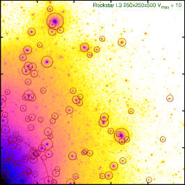
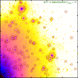
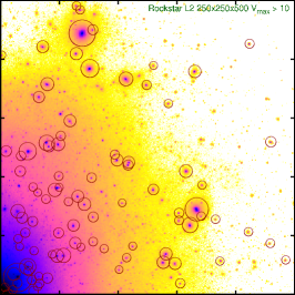
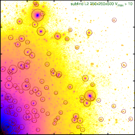
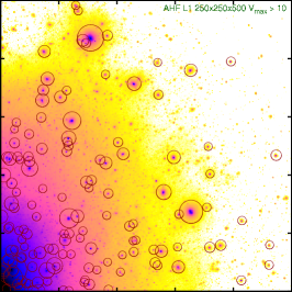
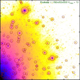
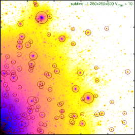
Figure 2: Subhalo recovery as a function of resolution. Location and size of recovered substructure from level 3 to level 1 for the three finders that reached this level. In all panels subhaloes with $v_{\rm max}$$>10$ km/s are shown, scaled by $v_{\rm max}$ as in Figure 1 and the background image is the smoothed dark matter density at that level. The relevant finder and level are labelled in the top right of each panel. The biggest change between levels is the additional small scale power moving the substructure locations.

3 The Data

The data used for this paper forms part of the Aquarius project (Springel et al., 2008). It consists of multiple dark matter only re-simulations of a Milky Way like halo at a variety of resolutions performed using gadget3 (based on gadget2, Springel, 2005). We have used the Aquarius-A halo dataset at $z=0$ for this project. This provides 5 levels of resolution, varying in complexity from the 2.3 million particles of the lowest resolution (i.e. level 5), up to the 4.25 billion particles of the highest resolution (i.e. level 1), as shown in Table 1. The underlying cosmology for the Aquarius simulations is the same as that used for the Millennium simulation (Springel et al., 2005) i.e. $\Omega_{M}=0.25,\Omega_{\Lambda}=0.75,\sigma_{8}=0.9,n_{s}=1,h=0.73$. These parameters are consistent with the latest WMAP data (Jarosik et al., 2011) although $\sigma_{8}$ is a little high. All the simulations were started at an initial redshift of 127. Precise details on the set-up and performance of these models can be found in Springel et al. (2008).

The participants were asked to run their subhalo finders on the supplied data and to return a catalogue listing the substructures they found. Specifically they were asked to return a list of uniquely identified substructures together with a list of all particles associated with each subhalo.

Finders were initially run on the smallest dataset, the Aq-A-5 data. This allowed for debugging of the common output format required by the project and some basic checks on the internal consistency of the data returned from each participant. Once this had been achieved each participant scaled up to the higher resolution datasets, continuing until they reached the limits of their finder and/or the computing resources readily available to them. A summary of the number of subhaloes found by each subhalo finder at the various levels is contained in Table 2 as well as the size of the largest subhalo at level 4. All of the finders that participated in this study completed the analysis of the level 4 dataset which is used for the main comparison that follows and contains around 6 million particles within the region considered, a sphere of radius 250 kpc/$h$ around a fiducial centre. Three of the finders (ahf, rockstar & subfind) completed the analysis of the very computationally demanding level 1 dataset. In addition to these hbt and hsf completed level 2 which contains around 160 million particles within the region examined here.

Table 1: Summary of key numbers for each Aquarius level, the dataset used for this study. $N_{h}$ is the number of particles with the highest resolution (lowest individual mass). $N_{l}$ the number of low resolution particles - the sum of the remainder. $N_{250}$ is the number of high resolution particles found within a sphere of radius 250 kpc/h from the fiducial centre at each resolution (i.e. those of interest for this study). $M_{p}$ is the mass of one of these particles (in $\mathrm{M_{\sun}/h}$). $S$ is the resolution increase (mass decrease) for each level relative to level 5, and $S_{p}$ is the resolution increase relative to the previous level. All particles are dark matter particles.

Data	$N_{h}$	$N_{l}$	$N_{250}$	$M_{p}$	$S$	$S_{p}$
Aq-A-5	2,316,893	634,793	712,232	$2.294\times 10^{6}$	1	$\times 1$
Aq-A-4	18,535,972	634,793	5,715,467	$2.868\times 10^{5}$	8	$\times 8$
Aq-A-3	148,285,000	20,035,279	45,150,166	$3.585\times 10^{4}$	64	$\times 8$
Aq-A-2	531,570,000	75,296,170	162,527,280	$1.000\times 10^{4}$	229	$\times 3.6$
Aq-A-1	4,252,607,000	144,979,154	1,306,256,871	$1.250\times 10^{3}$	1835	$\times 8$

Table 2: The number of subhaloes containing 20 or more particles and centres within a sphere of radius 250kpc/h from the fiducial centre found by each finder after standardised post-processing (see Section 4.1). Three finders (ahf, rockstar & subfind) returned results from the highest resolution (level 1) within the timescale of this project. Below this we list the number of particles contained within the largest subhalo after post-processing.

	Number of subhaloes within 250kpc/h of the fiducial centre after post processing.
Name	adaptahop	ahf	hbt	hot3d	hot6d	hsf	mendieta	rockstar	stf	subfind	voboz
Aq-A-5	353	230	228	58	136	231	207	272	205	214	257
Aq-A-4	2497	1599	1544	1265	1075	1544	1493	1707	1521	1433	1862
Aq-A-3	-	11213	11693	-	-	11240	10948	11797	10250	10094	13343
Aq-A-2	-	38441	39703	-	-	35445	-	38489	-	33135	-
Aq-A-1	-	226802	-	-	-	-	-	235819	-	221229	-
	Number of particles in the largest subhalo within 250kpc/h of the fiducial centre after post processing.
Aq-A-4	49076	77225	66470	69307	61581	73167	48387	78565	56990	50114	54685

Both the halo finder catalogues (alongside the particle ID lists) and our post-processing software (to be detailed below) are publically available from the web site http://popia.ft.uam.es/SubhaloesGoingNotts under the Tab “Data”.

4 The Comparison

We are going to primarily focus on comparing the location of subhaloes (both visually and quantitatively), the mass spectrum, and the distribution of the peak value of the rotation curve. The comparison, however, is based solely upon the provided particle lists and not the subhalo catalogues as the latter are based upon each code’s own definitions and means to determine aforementioned properties and hence possibly introducing “noise” into the comparison (cf. Knebe et al., 2011). In order to achieve a fair comparison between the respective finders we produced a single analysis pipeline which we used to post-process the particle lists provided by each participating group. This ensured consistency across our sample while removing differences due to the adoption of different post-processing methodologies and the particular choice of threshold criteria. The comparison detailed in this paper is restricted to this uniform post-processed dataset. We intend to explore differences due to different methodologies in a subsequent work. However, we stress at the outset that our particular chosen post-processing methodology is not intended to be unique nor do we put it forward as the best way of defining a subhalo. Rather we use a single methodology so that we can first answer the most fundamental question: if we agree on a single subhalo definition do the different finders agree on the most fundamental properties they recover? Perhaps surprisingly we will see that the answer to this question is broadly yes.

We did not consider in this paper efficiency of processing, as to make a fair comparison the codes would need to run on comparable machines with a set amount of memory and processors. In this instance the finders were run with the resources that were available to each of the participants. Some indication of the capabilities of the respective finders may be deduced from Table 2.

4.1 Post-processing pipeline

Some finders (e.g. ahf) include the mass (and particles) of a subhalo within the encompassing host halo whereas others do not (e.g. subfind), preferring each particle to only be associated with a single structure. Either of these approaches has its pros and cons. For instance, keeping the subhalo mass as part of the halo mass makes it straightforward to calculate the enclosed dynamical mass of any object. However, such an approach easily leads to multiple counting of mass, particularly if there are many layers of the substructure hierarchy. In principle though it is not difficult to transform from one definition to the other given knowledge of both the halo and particle locations. In our study, 5 of the 11 finders chose to include the mass of subhaloes whereas the other 6 did not. Following our principle of creating a uniform analysis pipeline we processed all the particle lists to ensure that a particle could only reside within a single structure. To this end, we first sorted the returned halo catalogue into mass order. Then starting from the smallest halo we performed the centring, trimming and overdensity checks detailed below to trim the subhalo uniformly. We then tagged the particles contained within this object as being within a subhalo before continuing to the next largest subhalo and repeating the procedure ignoring particles already tagged as being used before. This preserved the maximum depth of the subhalo hierarchy while ensuring that a particle could only reside within a single subhalo. We should remark that in practice excising all the sub-subhaloes from each subhalo’s particle list made little difference to any of the results presented here as at any level of the subhalo hierarchy only around 10 per cent of the material is within a subhalo of the current halo. So sub-subhaloes contribute only around 1 per cent of the halo mass, although it can affect other properties such as the centre of mass.

All the particles belonging to the list each finder identified as being associated with a subhalo were extracted from the original simulation data files to retrieve each particle’s position, velocity and mass. From this data the centre of mass was first calculated, before being refined based on consideration of only the innermost 10 per cent of these particles, sorted with respect to the initial centre of mass. This procedure was repeated until a stable centre was found, i.e. until the change in the position was below the actual force resolution of the simulation. Once the centre had been defined the particles were ordered radially from this point and a rotation curve $GM(<r)/r$ and overdensity $M(<r)/(4\pi r^{3}/3)$ calculated until it dropped below 200 times the critical density $\rho_{\rm crit}$ defining the subhalo radius $R_{200}$ and mass $M_{200}$. All particles outside $R_{200}$ were removed which was essential in particular for the phase-space finders who also considered already stripped material as still being part of and belonging to the subhalo. Please note that our post-processing pipeline does explicitly not feature an unbinding procedure as this already formed part of most halo finding algorithms. At this point the maximum circular velocity, $v_{\rm max}$ was obtained by smoothing the rotation curve and locating its maximum by searching both inwards and outwards for a peak in the rotation curve and taking the average of these two measures, a process that stabilises the measure if the rotation curve is very flat or noisy.

We emphasise that the precise subhalo properties are somewhat sensitive to the definition of the halo centre. Various groups use the centre-of-mass as the centre of all material enclosed within the subhalo’s radius (both with and without including substructure), the centre-of-mass of some smaller subset (as here for example), the location of the most bound particle, the location of the densest particle or the minimum of the gravitational potential. Additionally different groups use different methodologies for deciding whether or not a particle is bound to a halo as this involves some decisions about the global potential and can be a very time consuming process if done fully generally and iteratively.

Finally the choice of where to place the subhalo edge is also problematic. By definition the subhalo resides within some in-homogeneous background density and so at some point particles cease to belong to it and should rather be associated with the background object. Different groups split the host halo from the subhalo in different ways and there is no correct method. Without a uniform choice these differences can swamp any differences due to actually finding subhaloes or not. We stress that our post-processing (where we treat each subhalo in isolation) can only remove particles from the original list of those particles associated with a subhalo. We have therefore tested whether or not our results are sensitive to our choice of 200 as an overdensity parameter by re-running our analysis with a tighter threshold of 500. Other than making all the subhalo masses smaller this has no noticeable effect on the scatter of the cumulative number counts. We therefore decided to stick to the original choice of $R_{200}$ and $M_{200}$, respectively. Further, throughout the subsequent comparison only haloes with more than 20 (bound) particles within $R_{200}$were used, although some finders detected and returned haloes with less particles.

To summarise, our uniform post-processing pipeline involved the following steps, applied iteratively where necessary:

• The subhalo catalogues were sorted into mass order.

• Starting from the smallest subhalo, the particles associated with the current subhalo were obtained from the simulation data.

• Only particles tagged as “not used before” were considered.

• The centre-of-mass was iteratively calculated using the innermost 50 per cent of particles. (Originally we used the innermost 10 per cent but found some of the more dispersed sub structures did not converge with this value).

• A value for $R_{200}$ was calculated based on an enclosed overdensity of 200 times the critical density.

• The subhalo mass and rotation curve peak $v_{\rm max}$ were computed based on particles inside $R_{200}$.

• Only substructures containing more than 20 particles were retained.

4.2 Visual comparison

A visual representation of the location and size (based on $v_{\rm max}$) of the recovered subhaloes at Aquarius level 4 from each of the finders is shown in Figure 1. A smoothed colour image of the underlying dark matter density based on all particles from the original Aquarius data are shown in one quadrant of the main halo, and this is overplotted with the recovered subhaloes from each finder indicated by circles whose size is scaled according to $v_{\rm max}$ (specifically $v_{\rm max}$ (in km/s) divided by 3). This allows a visual comparison between the finders. Only haloes with $v_{\rm max}$ $>10h^{-1}$km/s are shown. We immediately see that most of the finders are very capable of extracting the locations of the obvious overdensities in the underlying dark matter field. Wherever you would expect to find a subhalo (given the background density map) one is indeed recovered. This demonstrates that substructure finders should be expected to work well, recovering the vast majority of the substructure visible to the eye. Additionally, if our aforementioned post-processing is applied the quantitative agreement between the finders is also excellent, with the extracted structures having very similar properties between finders (see below). The majority of the finders agree very well, reliably and consistently recovering nearly all the subhaloes with maximum circular velocities above our threshold.

While Figure 1 illustrates the agreement between the finders at a single Aquarius level (in this case level 4, which all the participating finders have completed), in Figure 2 we construct a similar Figure to illustrate the agreement between levels. We show the same quadrant at level 3 to level 1 for the three finders that have completed the level 1 analysis (i.e., ahf, rockstar & subfind); we deliberately omitted level 5 and level 4 as the former is not very informative and the latter has already been presented in Figure 1. As can be seen, the main difference between the different levels is in the exact location of the substructures. This changes because additional power was added to the Aquarius initial power spectrum to produce the additional small objects that form as the resolution is increased (fundamentally, the Nyquist frequency has changed as there are more available tracers within the higher resolution box). This extra power moves the substructure around slightly, and these differences are amplified in the, by definition, non-linear region of a collapsed object. Despite this the ready agreement between the three finders at any single level is clear to see and this is similarly true for both the other finders (hbt, hsf) that completed level 2. We do not explore the effect of changing the resolution on subhalo extraction in more detail here because that is not the main point of this paper, which focuses on how well different finders extract substructure relative to each other. Also, this topic has already been well studied for subfind using this same suite of models by (Springel et al., 2008).

4.3 Subhalo Mass Function

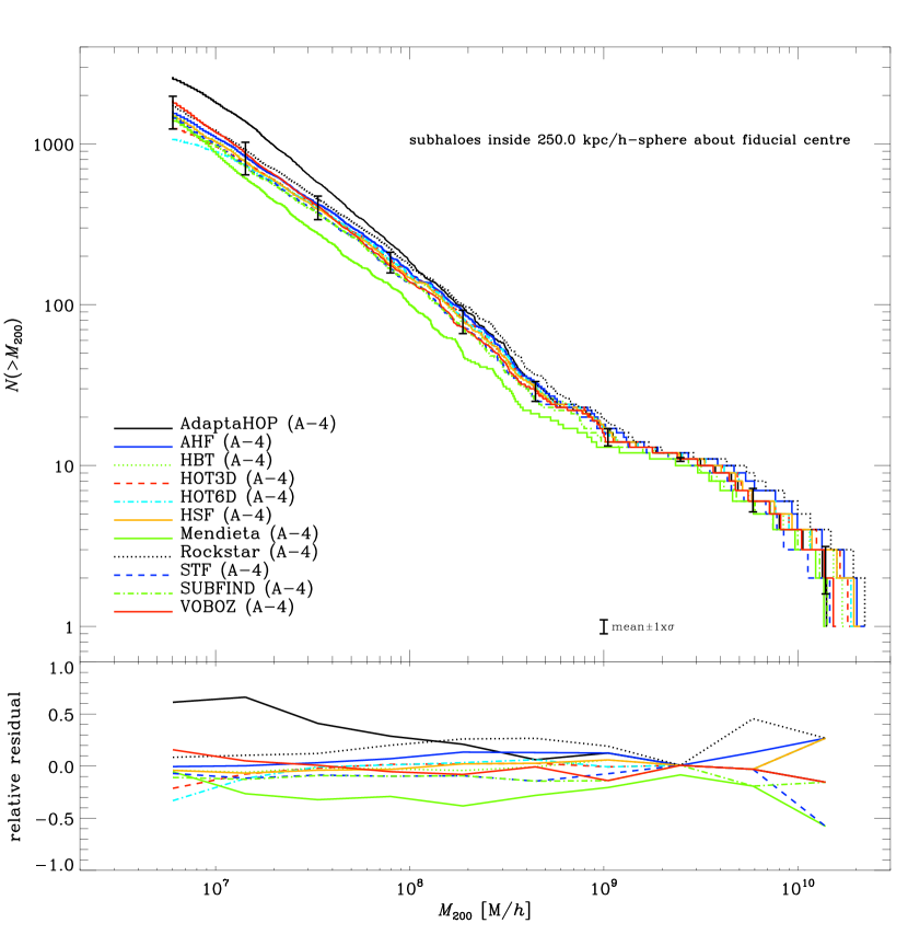
Figure 3: Cumulative number count of subhaloes above the indicated mass found ($M_{200}$) within a radius of 250 kpc/h from the fiducial halo centre after standardised post-processing at resolution level 4 (see Section 4.1 for details). The bottom plot shows the relative offset from the mean of the cumulative mass curve.

4.3.1 Level 4

Perhaps the most straightforward quantitative comparison is simply to count the number of subhaloes found above any given mass. For Aquarius level 4 this produces the cumulative mass plot (based on $M_{200}$) shown in Figure 3. Results from each participating finder are shown as a line of the indicated colour. Generally the agreement is good, with some intrinsic scatter and a couple of outliers (particularly adaptahop and mendieta) which do not appear to be working as well as the others, finding systematically too many or too few subhaloes of any given mass respectively. For adaptahop we like to remind the reader that this code does not feature a procedure where gravitationally unbound particles are removed; we therefore expect lower mass haloes stemming from Poisson noise in the background host halo to end up in the halo catalogue as well as haloes to have a higher mass in general possibly explaining the distinct behaviour of this code. But typically the scatter between codes is around the 10 per cent level except at the high mass end where it is larger as each finder systematically recovers larger or smaller masses in general. We like to remind the reader again that this scatter is neither due to the inclusion/exclusion of sub-subhaloes (which has been taken care of by our post-processing pipeline) nor the definition of the halo edge: as the 10 per cent differences still remain if choosing $R_{500}$ as the subhalo edge.

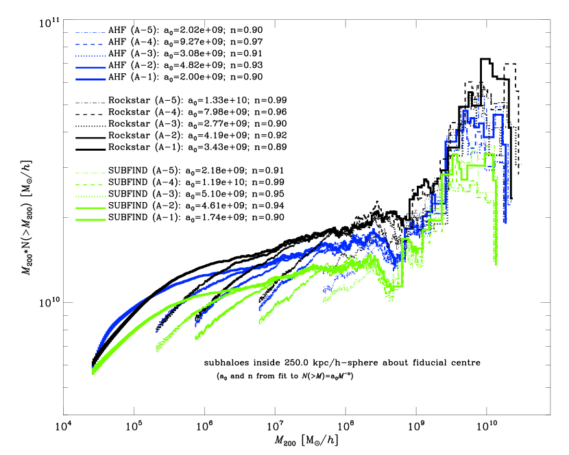
Figure 4: Cumulative subhalo mass function (multiplied by $M$ to compress the vertical dynamical range) for all five Aquarius levels for the ahf, rockstar, and subfind finder. We fit the function $N(>M)/N_{\rm tot}=a_{0}\times M^{-n}$ between the mass equivalent to 100 particles at each level and $10^{9}\mathrm{M_{\sun}/h}$. Note: the data has not been shifted for clarity but is as plotted.

Table 2 lists the number of subhaloes found that contain 20 or more particles after the uniform post-processing procedure detailed above had been performed and within $250$ kpc/h of the fiducial centre of the main Aquarius halo at each level completed for all the eleven finders that participated. These number counts are generally remarkably consistent, again with a few outliers as expected from Figure 3. The majority of the finders are recovering the substructures remarkably well and consistent, respectively.

As an additional quantitative comparison we list the number of particles associated with the largest substructure found by each of the finders as the last row of Table 2. All the finders recover a structure containing $60,000$ particles $\pm 20$ per cent. As Figure 3 has shown there is a lot of residual scatter for the highest mass haloes even when a uniform post-processing pipeline is used. This is most likely due to the different unbinding algorithms used in the initial creation of the substructure membership lists which are particularly uncertain for these large structures. At the other end of the substructure mass scale we have chosen to truncate our comparison at subhaloes containing 20 particles as this was shown to be the practical limit in Knebe et al. (2011). Some participants returned haloes smaller than this as this is their normal practice. They all stress that such small subhaloes should be treated with extreme caution but that there does appear to be a bound object at these locations even if its size is uncertain. We have removed them here for the purposes of a fair comparison.

Other plots that could be considered are those comparing the number of subhaloes against radial distance, or fractional mass against radial distance. Both these were produced and considered, but did not give any further insight to the comparison.

4.3.2 All Levels

Cumulative subhalo number counts like that shown for level 4 in Figure 3 can be calculated for all completed levels and compared. As shown in Figure 2 while increasing the resolution does not exactly reproduce the same substructures a reasonable approximation is achieved and so we expect to find a set of similar subhaloes containing more particles as we decrease the individual particle mass between levels (i.e. any specific subhalo should effectively be better resolved as the resolution increases). We show the cumulative number counts for the finders ahf, rockstar, and subfind (multiplied by $M$ to compensate for the large vertical scale) from level 5 to level 1 in Figure 4. We show this as an example and stress that similar plots with similar features could be produced for any of the finders that completed level 2. The curve for each level starts at 20 particles per halo and we like to stress that no artificial shifting has been applied: any differences seen in the plot are due to the different halo finding algorithms. Below about 100 particles per halo the cumulative number counts fall below the better resolved curves, indicating that subhaloes containing between 20 and 100 particles are not fully resolved and should have a slightly higher associated mass, also reported in Muldrew et al. (2011). Above $10^{9}\mathrm{M_{\sun}/h}$ the power law slope breaks as there are less than 10 subhaloes more massive than this limit and the number of these is a property of this particular host halo. For these reasons we fit a power law of the form

$$\frac{N(>M)}{N_{\rm tot}}=a_{0}M^{-n}$$ (1)

between 100 particles and $10^{9}\mathrm{M_{\sun}/h}$ where the power law breaks. Here $a_{0}$ is a normalisation (capturing the rise in the number of subhaloes due to the increase in resolution), $M$ is the mass and $n$ is the power law slope. The fitted values of the parameters by level are given in the legend for each finder. The subhalo cumulative number count appears to be an unbroken power law – at least in the range considered for the fitting. Similar results for subfind were found by Springel et al. (2008).

We extended this particular analysis of fitting a single power-law to the (cumulative) subhalo mass function to all finders at all available levels and compare the values of $a_{0}$ and $n$ as a function of level for all participating substructure finders in Figure 5. There we find that at level 5 little can be said because the fitting range is so narrow. At the lower, better resolved levels good agreement is seen between the finders (clearly adaptahop is a strong outlier on this plot, probably due to its lack of unbinding as mentioned before when discussing Figure 3, and hot3d (as well as the first resolution step of mendieta) is inverted with respect to the main trend) and a consistent trend emerges: all agree that the power law slope, $n$ is less than 1 and if anything decreasing with increasing resolution. Values of $n$ less than 1 are significant because they imply that not all the mass is contained within substructures, with some material being part of the background halo. This has important ramifications for studies requiring the fraction of material within substructures such as the dark matter annihilation signal and lensing work. Although this result is robust between all high-resolution finders we remind the reader that this is for a single halo within a single cosmological model. However, it does indicate that, as perhaps expected, the most important contribution to substructure mass is from the most massive objects and that progressively smaller structures contribute less and less to the signal.

4.4 Distribution of $v_{\rm max}$

If, instead of quantifying the total mass of each subhalo, we rather use the maximum rotational velocity, $v_{\rm max}$ to rank order the subhaloes in size we obtain a generally much tighter relation (see below). Knebe et al. (2011) already found that $v_{\rm max}$ was a particularly good metric for comparing haloes and we confirm this for subhaloes. As Muldrew et al. (2011) showed in figure 6 of their paper, this is because for an NFW profile (Navarro et al., 1997) the maximum of the rotation curve is reached at less than 20 per cent of the virial radius for objects in this mass range so $v_{\rm max}$ is a property that depends upon only the very inner part of the subhalo and is not affected by any assumptions made about the outer edge. On the other hand, it has also been shown (Ascasibar & Gottlöber, 2008) that $v_{\rm max}$ provides a meaningful tracer of the depth of the gravitational potential (i.e. the mass scale) of the halo.

Figure 6 displays the cumulative $v_{\rm max}$ for all the finders for level 4 again. All the finders align incredibly well for the largest subhaloes with $v_{\rm max}$$>$ 20 km/s. For subhaloes smaller than this the alignment remains tighter than the total mass comparison down to rotation velocities of around 6 km/s. At level 4 haloes of this size contain around 80 particles in total, so $v_{\rm max}$ is being calculated from less than 20 particles at this point; the arrows give an indication of the number of particles inside $r_{\rm max}$. adaptahop, despite its missing unbinding procedure, agrees well with other finders for high rotation velocities as this particular statistic probes inner regions of the subhaloes which are less affected by unbound particles; and its deviation at the lower $v_{\rm max}$-end is due to the existence of (small mass) fluke objects not removed by such an unbinding step.

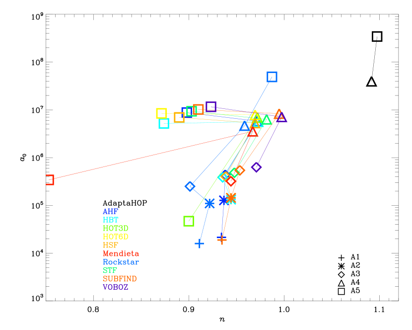
Figure 5: A comparison of the slope and normalisation of the fits of the mass function derived as per Figure 4 for all finders at all levels returned.

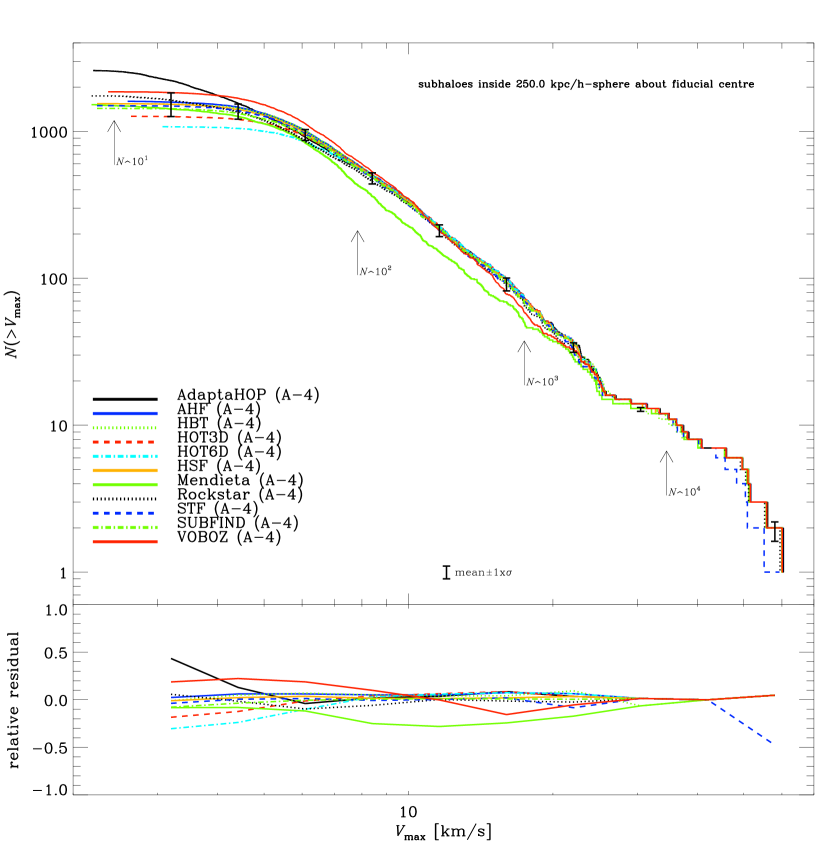
Figure 6: Cumulative number count of subhaloes above the indicated $v_{\rm max}$ value within a radius of 250 kpc/h from the fiducial halo centre after standardised post-processing (see Section 4.1). The arrows indicate the number of particles interior to $r_{\rm max}$, the position of the peak of the rotation curve. The bottom plot shows the relative offset from the mean of the cumulative count.

4.5 Radial Mass Distribution

The accumulated total mass of material with subhaloes is measured by ordering the subhalo centres in radial distance from the fiducial centre of the halo and summing outwards,i.e. $\sum_{r_{\rm sat}<r}M_{\rm sat}$. We include all post-processed subhaloes above our mass threshold of 20 particles. As Figure 7 demonstrates at level 4 most of the finders (ahf, hbt, hot6d, hsf, stf, voboz) agree very well, finding very similar amounts of substructure both in radial location and mass. rockstar finds a little more structure, particularly in the central region where its phase-space nature works to its advantage and subfind finds around a factor of 25 per cent less due to its conservative subhalo mass assignment.

The mendieta finder appears to show significantly different results to the rest. As previously noted the adaptahop finder locates many small subhaloes and these push up the total mass found in substructure above that found by the others particular in the range around 50-100kpc. We note that two of the three phase-space based finders (hot6d, & hsf) have a radial performance indistinguishable from real-spaced based finders. The only one to show any difference is rockstar and it remains unclear whether or not this is in practice a significant improvement.

We further like to mention (though not explicitly shown here) that a visual comparison akin to Figure 1 but focusing on the central 20 $h^{-1}$kpc reveals that it is very likely that the excess mass found in that inner region by some of the finders such as hot3d may be due to mis-identifications of the host halo as subhaloes. In the very central region it is difficult for the underlying real-space Friends-of-Friends methodology to distinguish structures from the background halo and so can show up either as multiple detections, or no structure at all.

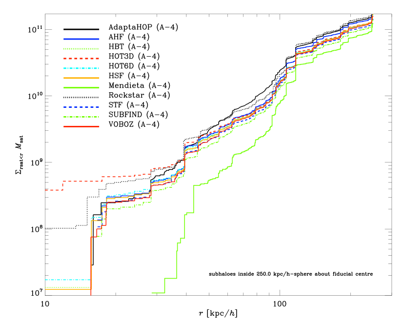
Figure 7: Cumulative plot of the enclosed mass within subhaloes as a function of radial distance from the fiducial centre of the host halo.

5 Summary & Conclusions

We have used a suite of increasing resolution models of a single Milky Way sized halo extracted from a self-consistent cosmological simulation (i.e. the Aquarius suite (Springel et al., 2008)) to study the accuracy of substructure recovery by a wide range of popular substructure finders. Each participating group analysed independently as many levels of the Aquarius-A dataset at redshift $z=0$ as they could manage and returned lists of particles they associated with any subhalo they found. These lists were post-processed by a single uniform analysis pipeline. This pipeline employed a standard fixed definition of the subhalo centre and subhalo mass, and employed a standard methodology for deriving $v_{\rm max}$. This analysis was used to produce cumulative number counts of the subhaloes and examine how well each finder was able to locate substructure.

We find a remarkable agreement between the finders which are based on widely different algorithms and concepts. The finders agree very well on the presence and location of subhaloes and quantities that depend on this or the inner part of the halo are amazingly well and reliably recovered. We agree with Knebe et al. (2011) that $v_{\rm max}$ is a good parameter by which to rank order the haloes (in this case subhaloes). However, we also show that as $v_{\rm max}$ is only dependent upon the inner 20 per cent or less of the subhalo particles around 100 particles are required to be within the subhalo for this measure to be reliably recovered. Quantities that depend on the outer parts of the subhaloes, such as the total mass, are still recovered with a scatter of around 10 per cent but are more dependent upon the exact algorithm employed both for unbinding (intrinsic to each finder) and to define the outer edge (given by the common post-processing applied here).

The most difficult region within which to resolve substructures is the very centre of the halo which has, by definition, a very high background density. In this region real-space based finders are expected to struggle whereas the full six-dimensional phase-space based finders should do better. In practice rockstar is the only phase-space based finder that shows any indication of this (and this difference becomes less pronounced as the resolution is increased); but we cannot rule out mis-identifications of the host halo as subhaloes at this stage. We conclude that, as yet, none of the phase-space based finders present a significant improvement upon the best of the more traditional real-space based finders.

Convergence studies indicate that identified subhaloes containing less than 100 particles tend to be under-resolved and these objects grow slightly in mass if a higher resolution study is used. This could be due to the fact that particles in the outer regions of these subhaloes are stripped more readily at lower resolution or it could be an artefact of the difficulty of measuring the potential (and hence completing any unbinding satisfactorily) with this small number of particles. Several studies (Kase et al., 2007; Pilipenko et al., 2009; Trenti et al., 2010) have indicated the unreliability of halo properties (other than physical presence) for (sub)haloes of this size or less.

Fitting power law slopes to the convergence studies of each finder indicates that the logarithmic slope of the cumulative number count is less than 1. While this is only confirmed for a single halo within a single cosmology, and ignoring any mass in tidal streams, the result appears to be robust as it is found for all the high-resolution finders employed in this study. This indicates that the larger substructures are the most important ones and that higher levels of the (sub)subhalo hierarchy play a less significant dynamical role.

We like to close with a brief note on the removal of gravitationally unbound particles for subhaloes. We have seen that the omission of such a procedure most certainly leads to rather distinct results. However, we cannot convincingly deduce whether or not this will lead to more small mass objects (as is the case for adaptahop) or to objects more massive in general (also seen for adaptahop), likely both will occur. But we confirm that the exact differences between a subhalo catalogue based upon a halo finding method with and without unbinding depend on the actual algorithm to collect the initial set of particles to be considered part of the subhalo: we performed an analysis of the level 4 data with ahf switching the unbinding part off ending up with a subhalo mass function that was only different at the higher mass end (not shown here though) as opposed to the adaptahop results; but both these codes differ substantially in the way of assigning the primary particle set to a subhalo.

It should be noted that the Aquarius-A halo is a relatively quiescent halo (Wang et al., 2011), not having been subject to many mergers. Investigation of other haloes, and those produced by other simulation code would be interesting to compare. Therefore more studies focusing on the actual halo catalogues returned by each finder (as opposed to the particle lists used here); other cosmological simulations and different simulated scenarios (such as disrupted galaxies); the detailed analysis of sub-substructure (which is only really practical at level 1); and other subhalo properties such as spin parameter and shape, as well as more detailed resolution studies for those codes providing an analysis of all levels will be deferred to future papers.

References

- Angulo et al. (2009) Angulo R. E., Lacey C. G., Baugh C. M., Frenk C. S., 2009, MNRAS, 399, 983
- Ascasibar (2010) Ascasibar Y., 2010, Comput. Phys. Commun., 181, 1438
- Ascasibar & Binney (2005) Ascasibar Y., Binney J., 2005, MNRAS, 356, 872
- Ascasibar & Gottlöber (2008) Ascasibar Y., Gottlöber S., 2008, MNRAS, 386, 2022
- Behroozi et al. (2011) Behroozi P. S., Wechsler R. H., Wu H.-Y., 2011, ArXiv preprint arXiv:1110.4372
- Boylan-Kolchin et al. (2011a) Boylan-Kolchin M., Bullock J. S., Kaplinghat M., 2011a, ArXiv preprint arXiv:1111.2048
- Boylan-Kolchin et al. (2011b) Boylan-Kolchin M., Bullock J. S., Kaplinghat M., 2011b, MNRAS, 415, L40
- Boylan-Kolchin et al. (2009) Boylan-Kolchin M., Springel V., White S. D. M., Jenkins A., Lemson G., 2009, MNRAS, 398, 1150
- Contini et al. (2011) Contini E., De Lucia G., Borgani S., 2011, ArXiv preprint arXiv:1111.1911
- Cooper et al. (2010) Cooper A. P., Cole S., Frenk C. S., White S. D. M., Helly J., Benson A. J., De Lucia G., Helmi A., Jenkins A., Navarro J. F., Springel V., Wang J., 2010, MNRAS, 406, 744
- De Lucia et al. (2004) De Lucia G., Kauffmann G., Springel V., White S. D. M., Lanzoni B., Stoehr F., Tormen G., Yoshida N., 2004, MNRAS, 348, 333
- di Cintio et al. (2011) di Cintio A., Knebe A., Libeskind N. I., Yepes G., Gottlöber S., Hoffman Y., 2011, MNRAS, 417, L74
- Diemand et al. (2008) Diemand J., Kuhlen M., Madau P., Zemp M., Moore B., Potter D., Stadel J., 2008, Nat, 454, 735
- Elahi et al. (2011) Elahi P. J., Thacker R. J., Widrow L. M., 2011, MNRAS, 418, 320
- Ferrero et al. (2011) Ferrero I., Abadi M. G., Navarro J. F., Sales L. V., Gurovich S., 2011, ArXiv preprint arXiv:1111.6609
- Freeman & Bland-Hawthorn (2002) Freeman K., Bland-Hawthorn J., 2002, ARA&A, 40, 487
- Gao et al. (2004) Gao L., White S. D. M., Jenkins A., Stoehr F., Springel V., 2004, MNRAS, 355, 819
- Gill et al. (2004) Gill S. P., Knebe A., Gibson B. K., 2004, MNRAS, 351, 399
- Gill et al. (2004) Gill S. P. D., Knebe A., Gibson B. K., Dopita M. A., 2004, MNRAS, 351, 410
- Han et al. (2011) Han J., Jing Y. P., Wang H., Wang W., 2011, Arxiv preprint arXiv:1103.2099
- Hernquist (1990) Hernquist L., 1990, ApJ, 356, 359
- Jarosik et al. (2011) Jarosik N., Bennett C. L., Dunkley J., Gold B., Greason M. R., Halpern M., Hill R. S., Hinshaw G., Kogut A., Komatsu E., Larson D., Limon M., Meyer S. S., Nolta M. R., Odegard N., Page L., Smith K. M., Spergel D., Tucker G. S., Weiland J. L., Wollack E., Wright E. L., 2011, ApJS, 192, 14
- Kase et al. (2007) Kase H., Makino J., Funato Y., 2007, PASJ, 59, 1071
- Klypin et al. (1999) Klypin A., Gottlöber S., Kravtsov A. V., Khokhlov A. M., 1999, ApJ, 516, 530
- Klypin et al. (1999) Klypin A., Kravtsov A. V., Valenzuela O., Prada F., 1999, ApJ, 522, 82
- Klypin et al. (2011) Klypin A. A., Trujillo-Gomez S., Primack J., 2011, ApJ, 740, 102
- Knebe et al. (2005) Knebe A., Gill S. P. D., Kawata D., Gibson B. K., 2005, MNRAS, 357, L35
- Knebe et al. (2011) Knebe A., Knollmann S. R., Muldrew S. I., Pearce F. R., Aragon-Calvo M. A., Ascasibar Y., Behroozi P. S., Ceverino D., Colombi S., Diemand J., 2011, MNRAS, pp 819–
- Knollmann & Knebe (2009) Knollmann S. R., Knebe A., 2009, ApJS, 182, 608
- Kuhlen et al. (2008) Kuhlen M., Diemand J., Madau P., 2008, ApJ, 686, 262
- Libeskind et al. (2011) Libeskind N. I., Knebe A., Hoffman Y., Gottlöber S., Yepes G., 2011, MNRAS, 418, 336
- Maciejewski et al. (2009) Maciejewski M., Colombi S., Springel V., Alard C., Bouchet F. R., 2009, MNRAS, 396, 1329
- Maciejewski et al. (2011) Maciejewski M., Vogelsberger M., White S. D. M., Springel V., 2011, MNRAS, 415, 2475
- Moore et al. (1999) Moore B., Ghigna S., Governato F., Lake G., Quinn T., Stadel J., Tozzi P., 1999, ApJ, 524, L19
- Muldrew et al. (2011) Muldrew S. I., Pearce F. R., Power C., 2011, MNRAS, 410, 2617
- Navarro et al. (1997) Navarro J. F., Frenk C. S., White S. D. M., 1997, ApJ, 490, 493
- Neyrinck et al. (2005) Neyrinck M. C., Gnedin N. Y., Hamilton A. J. S., 2005, MNRAS, 356, 1222
- Oh et al. (2011) Oh S.-H., Brook C., Governato F., Brinks E., Mayer L., de Blok W. J. G., Brooks A., Walter F., 2011, ApJ, 142, 24
- Pilipenko et al. (2009) Pilipenko S., Doroshkevich A., Gottlöber S., 2009, Astronomy Reports, 53, 976
- Pontzen & Governato (2011) Pontzen A., Governato F., 2011, ArXiv preprint arXiv:1106.0499
- Sgró et al. (2010) Sgró M. A., Ruiz A. N., Merchán M. E., 2010, BAAA, 53, 43
- Springel (2005) Springel V., 2005, MNRAS, 364, 1105
- Springel et al. (2008) Springel V., Wang J., Vogelsberger M., Ludlow A., Jenkins A., Helmi A., Navarro J. F., Frenk C. S., White S. D., 2008, MNRAS, 391, 1685
- Springel et al. (2008) Springel V., White S. D. M., Frenk C. S., Navarro J. F., Jenkins A., Vogelsberger M., Wang J., Ludlow A., Helmi A., 2008, Nat, 456, 73
- Springel et al. (2005) Springel V., White S. D. M., Jenkins A., Frenk C. S., Yoshida N., Gao L., Navarro J., Thacker R., Croton D., Helly J., Peacock J. A., Cole S., Thomas P., Couchman H., Evrard A., Colberg J., Pearce F., 2005, Nat, 435, 629
- Springel et al. (2001) Springel V., White S. D. M., Tormen G., Kauffmann G., 2001, MNRAS, 328, 726
- Stadel et al. (2009) Stadel J., Potter D., Moore B., Diemand J., Madau P., Zemp M., Kuhlen M., Quilis V., 2009, MNRAS, 398, L21
- Trenti et al. (2010) Trenti M., Smith B. D., Hallman E. J., Skillman S. W., Shull J. M., 2010, ApJ, 711, 1198
- Vogelsberger et al. (2009) Vogelsberger M., Helmi A., Springel V., White S., Wang J., Frenk C., Jenkins A., Ludlow A., Navarro J., 2009, MNRAS, 395, 797
- Wang et al. (2011) Wang J., Navarro J. F., Frenk C. S., White S. D. M., Springel V., Jenkins A., Helmi A., Ludlow A., Vogelsberger M., 2011, MNRAS, 413, 1373
- Warnick et al. (2008) Warnick K., Knebe A., Power C., 2008, MNRAS, 385, 1859
- White & Rees (1978) White S. D. M., Rees M. J., 1978, MNRAS, 183, 341
- Zavala et al. (2010) Zavala J., Springel V., Boylan-Kolchin M., 2010, MNRAS, 405, 593