On multiplicity correlations
in the STAR data

K. FIAŁKOWSKI, R. WIT

M. Smoluchowski Institute of Physics
Jagellonian University

30-059 Kraków, ul.Reymonta 4, Poland

The STAR data on the multiplicity correlations between narrow pseudorapidity bins in the pp and AuAu collisions are discussed. The PYTHIA 8.145 generator is used for the pp data, and a naïve superposition model is presented for the AuAu data. It is shown that the PYTHIA generator with default parameter values describes the pp data reasonably well, whereas the superposition model fails to reproduce the centrality dependence seen in the data. Some possible reasons for this failure and a comparison with other models are presented.

Keywords: RHIC, multiplicity correlations

1 Introduction

The STAR experiment at the RHIC accelerator has measured the dependence of the multiplicity correlations between the symmetric narrow pseudorapidity bins as a function of pseudorapidity distance for pp and AuAu data at 200 GeV in the nucleon-nucleon center-of-mass (CM) system [1]. The data were taken separately for different centrality classes in AuAu collisions. The authors noted that the HIJING model [2] describes reasonably well the pp data, but fails completely for the central AuAu data, whereas the predictions of the Parton String Model [3] lie closer to the AuAu data, but fail to describe the dependence on pseudorapidity distance in the pp data.

The AuAu data were discussed in the subsequent paper by Y.-L. Yan et al. [4], who compared them with the PACIAE model [5] based on the PYTHIA generator [6]. The model overestimates systematically the correlation strength, and the difference increases strongly with decreasing centrality.

The authors show also the predictions of three other models, which differ significantly from those of PACIAE model for most central events, but overestimate the correlations strength for semiperipheral events as strongly as PACIAE.

In this paper we compare the STAR data and the models mentioned above with the new version of PYTHIA generator [7] for the pp data and the naïve superposition model for the AuAu data. We have found that already with the default values of parameters the PYTHIA 8.145 generator describes reasonably well the pp data. On the other hand, the superposition model fails completely to describe the AuAu data. In particular, the centrality dependence of the correlation strength, which was weaker than in the data in the PACIAE model, is completely absent in our model.

In the next section we describe the procedures used in the STAR paper for pp and AuAu data, which subsequently are used by us to analyze the events generated by PYTHIA and the superposition model. In Section 3. we show the results, and we discuss them in Section 4. Some conclusions and perspectives are presented in the last section.

2 Definitions and procedures

A standard quantity describing the strength of correlations between the phase space bins $1$ and $2$ is the correlation coefficient $b$.

$$b=\frac{D^{2}_{12}}{D_{1}D_{2}}=\frac{\overline{n_{1}\cdot n_{2}}-\overline{n_{1}}\cdot\overline{n_{2}}}{\sqrt{(\overline{n_{1}^{2}}-\overline{n_{1}}^{2})(\overline{n_{2}^{2}}-\overline{n_{2}}^{2})}},$$ (1)

where $n_{1}$ and $n_{2}$ denote the multiplicities in bin $1$ and $2$, respectively. In the STAR data analysis the pseudorapidity bins of the width $0.2$ (placed symmetrically in the CM frame) were used. The distance between the bin centers ranged from $0.2$ to $1.8$.

It is well known that the correlation coefficients in hadron-hadron scattering increase with energy reflecting mainly the fact that the multiplicity distributions are much wider than Poissonian and their widths grow with energy. The STAR authors were mainly interested in the comparison of the correlation strength for different centrality classes in heavy ion collisions. These classes were defined by the range of multiplicity $N$ of charged particles with $p_{T}>0.15$ GeV/c in a control bin of unit width, disjunctive with the bins for which $b$ was measured (to be defined in Section 3).

The $b$ values calculated directly from the formula above reflect mainly the spread of the average multiplicities within each centrality class, which is quite large. The ranges of $N$ producing equal number of events in each class are approximately $>430$, $320-430$, $230-320$, $155-230$ and $90-155$ for the most central $0-10\%$, $10-20\%$, $20-30\%$, $30-40\%$ and $40-50\%$ events, respectively. The relation between $\overline{n_{i}}$ and $N$ is approximately given by the ratio of the bin widths: $\overline{n_{i}}=0.2N$, since $dN/d\eta$ is nearly flat.

Let us consider a distribution of a variable $n$ depending on the external parameter $N$ in such a way, that $\overline{n}=\alpha N$. It is well known that in such a case the dispersion may be separated into two parts: the first one averaging over this parameter, and the second one reflecting the spread of this parameter. The corresponding formula reads as follows:

$$D^{2}\leavevmode\nobreak\ =\leavevmode\nobreak\ <\overline{n^{2}}>-<\overline{n}>^{2}\leavevmode\nobreak\ =\leavevmode\nobreak\ <\overline{n^{2}}-\overline{n}^{2}>+<\overline{n}^{2}>-<\overline{n}>^{2}\leavevmode\nobreak\ =\leavevmode\nobreak\ <D^{2}(N)>+\alpha^{2}D_{N}^{2}.$$ (2)

Here the bar denotes averaging over the distribution of $n$ for given $N$, $<...>$ denotes averaging over $N$, and in the last term $D_{N}^{2}$ denotes the dispersion of $N$.

The authors of STAR performed a more involved procedure to separate the "dynamical" part of the correlation coefficient from the dominant "combinatorial" part. In each centrality class and for each distance between bins they calculated the averages $\overline{n_{i}}$, $\overline{n_{i}^{2}}$ and $\overline{n_{1}\cdot n_{2}}$ for each value of $N$ and fitted the dependence on $N$ within each class by the linear or quadratic formula:

$$\overline{n_{i}}\leavevmode\nobreak\ =\leavevmode\nobreak\ a_{i}+b_{i}\cdot N,\leavevmode\nobreak\ \leavevmode\nobreak\ \overline{n_{i}^{2}}\leavevmode\nobreak\ =\leavevmode\nobreak\ c_{i}+d_{i}\cdot N+e_{i}\cdot N^{2},\leavevmode\nobreak\ \leavevmode\nobreak\ \overline{n_{1}\cdot n_{2}}\leavevmode\nobreak\ =\leavevmode\nobreak\ c_{12}+d_{12}\cdot N+e_{12}\cdot N^{2}.$$ (3)

Using the fitted values of the parameters they calculated these averages for $N=\overline{N}$ and inserted them into the formula (1). A value of $b$ was obtained for each centrality class and each value of pseudorapidity bin separation.

One may note that the distributions of $n_{i}$ for fixed $N$ are narrow. We assume that

$$D^{2}(N)\leavevmode\nobreak\ \sim\leavevmode\nobreak\ \overline{n}(N).$$ (4)

It is easy to check that in such a case the procedure described above gives quite similar results as simple averaging of $b$ over the distribution of $N$ within each class.

Indeed, let us assume that the formula (4) holds for both (identical) distributions of $n_{1}$ and $n_{2}$, and a similar formula holds for $D_{12}^{2}$. Then the parameters of the fits (3) obey the following relations:

$$a_{1}\leavevmode\nobreak\ =\leavevmode\nobreak\ a_{2},\leavevmode\nobreak\ \leavevmode\nobreak\ b_{1}\leavevmode\nobreak\ =\leavevmode\nobreak\ b_{2},\leavevmode\nobreak\ \leavevmode\nobreak\ c_{1}\leavevmode\nobreak\ =\leavevmode\nobreak\ c_{2},\leavevmode\nobreak\ \leavevmode\nobreak\ d_{1}\leavevmode\nobreak\ =\leavevmode\nobreak\ d_{2},\leavevmode\nobreak\ \leavevmode\nobreak\ e_{1}\leavevmode\nobreak\ =\leavevmode\nobreak\ e_{2}\leavevmode\nobreak\ =\leavevmode\nobreak\ e_{12}\leavevmode\nobreak\ =\leavevmode\nobreak\ b_{1}^{2}.$$ (5)

Averaging separately $D_{12}^{2}(N)$ and $D_{1}^{2}=D_{2}^{2}=D_{1}D_{2}$ and inserting them into formula (1) we get in general

$$b=\frac{<D_{12}^{2}>}{<D_{1}^{2}>}=\frac{(e_{12}-b_{1}^{2})<N^{2}>+(d_{12}-2a_{1}b_{1})<N>+c_{12}-a_{1}^{2}}{(e_{1}-b_{1}^{2})<N^{2}>+(d_{1}-2a_{1}b_{1})<N>+c_{1}-a_{1}^{2}},$$ (6)

whereas from the STAR prescription we obtain

$$b^{\prime}=\frac{D_{12}^{2}(<N>)}{D_{1}^{2}(<N>)}=\frac{(e_{12}-b_{1}^{2})<N>^{2}+(d_{12}-2a_{1}b_{1})<N>+c_{12}-a_{1}^{2}}{(e_{1}-b_{1}^{2})<N>^{2}+(d_{1}-2a_{1}b_{1})<N>+c_{1}-a_{1}^{2}}.$$ (7)

As we see, these two formulae are equivalent when the conditions (5) are fulfilled.

For the pp data the STAR Collaboration measured the correlation coefficient $b$ for each value of bin separation $\Delta\eta$ and for each value of the multiplicity $N$ in the pseudorapidity range of two units. Then the result was averaged over the distribution of $N$. This amounts approximately to using the formula (6). In fact, all three prescriptions are approximately equivalent.

3 PYTHIA, superposition model and the data

To understand the physical meaning of the data presented by the STAR Collaboration it is useful to perform the same procedures on the events generated by a Monte Carlo generator. For pp collisions there are many models describing high energy data. We use here the PYTHIA 8.145 with the default value of parameters. We analyze the generated events in the same way as described above for the STAR data. We checked that the PYTHIA results are practically the same when we use the non-diffractive (ND) and the non-single-diffractive (NSD) samples of events.

In Fig.1 the STAR data at $E_{CM}=200$GeV and the model predictions for pp collisions are shown. The HIJING [2] and Parton String Model (PSM) [3] predictions are copied from the STAR paper [1]. The values of $b$ depend rather weakly on the bin separation $\Delta\eta$ and the HIJING and PYTHIA models describe them reasonably well, although the $\Delta\eta$ dependence seems to be too strong in HIJING and too weak in PYTHIA. The PSM model predicts practically no $\Delta\eta$ dependence, and seems to be incompatible with the data.

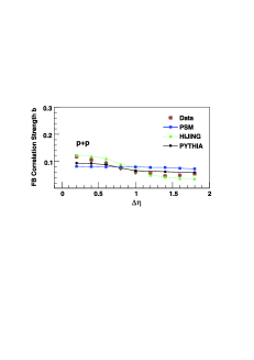
Figure 1: The correlation coefficients for the symmetric pseudorapidity bins of width $0.2$ for the distance between the bin centers ranging from $0.2$ to $1.8$. Full circles in open squares, squares, triangles and full circles denote data and the predictions of PSM, HIJING and PYTHIA models, respectively. Model predictions are connected by lines to guide the eye.

For AuAu collisions the situation is more involved. The centrality classes were defined by the multiplicity in a control pseudorapidity bin of the unit length, disjoint with the bins between which the correlation is measured. For the correlated bins $(-1,-0.8),\leavevmode\nobreak\ (0.8,1)$ and $(-0.8,-0.6),\leavevmode\nobreak\ (0.6,0.8)$ the control bin is $(-0.5,0.5)$; for the bins $(-0.2,0),\leavevmode\nobreak\ (0,0.2)$ and $(-0.4,-0.2),\leavevmode\nobreak\ (0.2,0.4)$ the control bin is made up of two parts: $(-1,-0.5)$ and $(0.5,1)$. For the bins $(-0.6,-0.4),\leavevmode\nobreak\ (0.4,0.6)$ the control bin consists of three parts: $(-1,-0.75),\leavevmode\nobreak\ (-0.25,0.25)$ and $(0.75,1)$. All the generated samples of events were divided into the equally populated centrality classes, as described in the previous section.

To generate a sample of AuAu events comparable with the data we used a naïve superposition model. In this model a heavy ion collision with $N_{part}$ nucleon participants from each nucleus is presented as a straight superposition of $N_{part}$ pp collisions, each generated by the PYTHIA. To reproduce a sample of events belonging to the fixed centrality class we use the known experimental multiplicity distribution in the control bin $P(N)$. The shape of the distribution of $N_{part}$ is assumed to be the same as that of $P(N)$, and the average value $<N_{part}>$ is chosen to reproduce the value of $<N>$ in this class.

In fact, the shape of $P(N)$ is nearly linear in $N$ for the large part of the distribution. Only for the most central part of the distribution ($0-10\%$) it falls down much faster (approximately Gaussian-like), and for the most peripheral events the maximum is sharper. This makes the generation of the $P(N_{part})$ quite easy. In Fig.2 the predictions from such a model for five classes of the most central events are presented on the right hand side plot. On the left hand side the STAR data for the same centrality classes are presented and compared with the results of the PACIAE model [5].

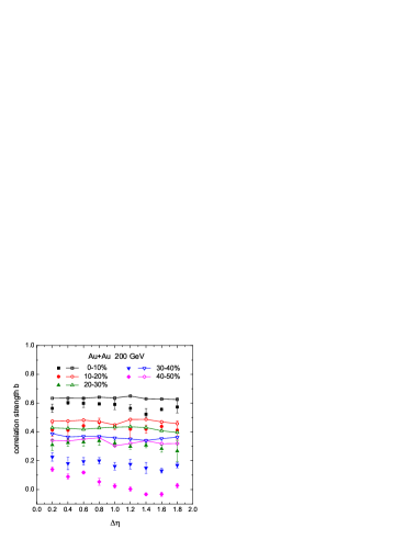
Figure 2: The correlation coefficients $b$ as a function of pseudorapidity distance $\Delta\eta$. On the left: the STAR data (full symbols) and PACIAE model (open symbols). Squares, circles, straight and inverted triangles and diamonds are used for the centrality classes 0-10%, 10-20%, 20-30%, 30-40% and 40-50%, respectively. On the right: our superposition model. The results for different centrality classes (marked as for the PACIAE model) are indistinguishable.

We see that none of the models describes the data properly. For the most central class of events the disagreement of the PACIAE model with data is not very bad, but it grows quickly for the more peripheral classes. The $\Delta\eta$ dependence of the correlation coefficient is rather weak and similar in the model and data. However, the dependence on the centrality is quite strong in the data and much weaker in the model. Our naïve model shows practically no dependence on centrality. Thus the disagreement with data is significantly worse. The $\Delta\eta$ dependence is similarly weak in the data and in the PACIAE model.

One may add that the authors of the PACIAE model compared the data also with other models [5]. The spread of their predictions is quite large and for most central events they bracket the data. However, the results for most peripheral data considered (the $40\%-50\%$ class) for all the models are much higher than the data, which exhibit in fact the negative values of the correlation coefficient $b$ for the most distant bins.

4 Discussion

We have seen that the pp data analyzed separately for the given multiplicity $N$ in the available pseudorapidity range and then averaged over the distribution of $N$ are reasonably well described by different models. Both the value of the correlation coefficient $b\approx 0.1$ and the weak dependence on the psudorapidity separation $\Delta\eta$ appear without any tuning.

We should remember that the procedure used by STAR was designed to remove the influence of the global multiplicity fluctuations from the correlation effects. In fact, for the standard inclusive definition of the correlation coefficient $b$ the dispersions in the numerator and denominator of formula (1) are dominated by these fluctuations. The value of $b$ is then twice bigger than $0.1$ and increases with the bin width. Thus a valid question is: what are the correlations measured by the STAR procedure?

To clarify this point, let us consider an oversimplified model where there are no correlations for a fixed value of $N$. Then the distribution of the multiplicity $n$ inside a narrow pseudorapidity bin of the width $y$ is given by the binomial distribution

$$P(n)={N\choose n}p^{n}(1-p)^{N-n};\leavevmode\nobreak\ p=\leavevmode\nobreak\ <n>/N.$$ (8)

The generating function of this distribution is

$$g(z)\equiv\sum_{n}z^{n}P(n)=(pz+1-p)^{N}.$$ (9)

Remember that the factorial moments of the distribution (8) are given by

$$<n_{q}>\leavevmode\nobreak\ \equiv\frac{n!}{(n-q)!}=\frac{dg(z)}{dz^{q}}\Bigg{|}_{z=1}=p^{q}N_{q}$$ (10)

It is easy to generalize these formulae for the case of two bins. The corresponding generating function is then

$$g(z_{1},z_{2})\equiv\sum_{n_{1},n_{2}}z_{1}^{n_{1}}z_{2}^{n_{2}}P(n_{1},n_{2})=[p(z_{1}+z_{2})+1-2p]^{N}.$$ (11)

The factorial moments for both bins can be calculated as in equation (10) and the average product of multiplicities as

$$<n_{1}n_{2}>\leavevmode\nobreak\ \equiv\frac{d^{2}g(z_{1},z_{2})}{dz_{1}dz_{2}}\Bigg{|}_{z_{1}=1,z_{2}=1}=p^{2}N(N-1).$$ (12)

This results in the simple formulae for the dispersions

$$D_{1}^{2}=D_{2}^{2}=p(1-p)N,\leavevmode\nobreak\ \leavevmode\nobreak\ D_{12}^{2}=-p^{2}N$$ (13)

and for the correlation coefficient

$$b=\frac{D_{12}^{2}}{D_{1}^{2}}=\frac{-p}{1-p}.$$ (14)

Since this formula does not depend on $N$, the averaging of $b$ over the distribution of $N$ will give the same result. This will not change if we average the numerator and denominator in (14) separately.

We see that this simplified model disagrees strongly with data: the values of $b$ are always negative, whereas in the data they are positive. Possible effects which introduce the positive correlations are:

• the existence of resonances, probably responsible for the dependence on $\Delta\eta$

• the existence of jets and minijets, possible dijet correlations

• the contribution of diffractive events (important for small $N$, decreasing for large $N$)

• Bose-Einstein interference, which may be important for adjacent bins.

Therefore we may conclude that the STAR procedure allows to measure the influence of these effects. They are significant, as they reverse the sign of the correlation coefficient. As indicated above, the realistic MC models describe them quite well.

For the AuAu collisions none of the considered models describes the data properly. The centrality dependence of the correlation coefficient $b$ seen in the data is significantly stronger than in the models. Moreover, our naïve model predicts practically no centrality dependence at all and thus the disagreement with the data is even worse than for other models.

Therefore one should ask what is the difference between our model and the other models. In our model it is assumed explicitly that the number of participating nucleons is the same in both colliding nuclei. It seems that this assumption suppresses the centrality dependence of the correlation coefficient.

This observation suggests that the data of STAR Collaboration, when interpreted within the superposition picture, measure mainly the fluctuations in the number of participating nucleons $N_{part}$ in both nuclei. For the most central class of events these fluctuations seem to be strongly correlated. With decreasing centrality this correlation becomes weaker both in the data and in the models.

One can understand this effect qualitatively in the framework of a "hidden asymmetry" picture [8], in which the dominant configuration is strongly asymmetric. There are few events in which the number of participants in both colliding nuclei is the same or similar. The correlation coefficient $b$ is positive and large for most central events, where the number of participants in both nuclei is nearly maximal (and thus approximately the same). The centrality is defined by the multiplicity in a symmetric control bin close to $\eta=0$. When this multiplicity decreases, the asymmetric configurations start to dominate, which results in decreasing values of $b$.

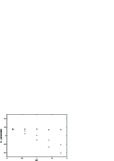
Figure 3: The correlation coefficients $b$ as a function of pseudorapidity distance $\Delta\eta$ for the $40-50\%$ class. Asterisks, triangles and circles are for the original model, triangular and flat distributions of $N_{F}$, respectively.

This is illustrated in Fig.3, where our toy model predictions for the $40-50\%$ class are compared with its two modified versions. In these versions the particles from each $p-p$ event generated by PYTHIA are divided randomly into the fragmentation products of two "wounded" nucleons. One of such "half-events" populates mainly the forward CM hemisphere and the other one backward one. The AuAu event is constructed from the (generally unequal) numbers of such half-events $N_{F}$ and $N_{B}$. For a given sum of these numbers we tried the distribution of $N_{F}$ to be flat or to have a triangular shape.

We see that it is quite easy to explain the decrease of $b$ with the pseudorapidity distance, even to the values much more negative than in the data. However, our model fails to explain the strong increase of $b$ for most central events and the adjacent bins.

This dependence may be reproduced qualitatively in PACIAE and other similar models, because they are not "pure" superposition models. The partons from initial nucleons interact forming the parton cascades which then hadronize. With increasing centrality the number of parton cascades increases. Apparently, the corresponding increase of the numerator in formula (1) is faster than the corresponding increase of the denominator.

However, the decrease for non-central events is underestimated in all the models. The negative values of $b$ in the data for the $40-50\%$ class, which correspond to the fact that for this class of events the positive fluctuation of $N_{part}$ in one nucleus is correlated with a negative fluctuation in the second nucleus, are not reproduced. This conforms with the idea of "hidden asymmetry". If asymmetric configurations are prevalent for semiperipheral events, the anticorrelation is natural.

5 Conclusions and outlook

The failure of superposition models is usually explained by the collective effects. An example of such an effect is the quark-gluon plasma formation, which should be most visible in the central events. However, the data for the most central $10\%$ of events are quite well described by the models where no plasma is formed [4]. As noted above, the biggest discrepancy is observed for semi-peripheral events. Other collective effects, as the hydrodynamical flow in the hadronic phase, are strongest for this class of events. On the other hand, it is not clear how such effects may be responsible for the discrepancy between the models and data. It seems more likely that the explanation is related to the "hidden asymmetry" of the interacting nucleons.

The negative correlation for the semiperipheral collisions are not the only unexpected feature of the STAR data. It was noted [9] that the large values of $b$ for the most central class of events suggest that the correlation between the distant bins "B" and "F" is stronger than the correlations between these bins and the central control bin. This contradicts the generally accepted feature of the uniform decrease of correlations with increasing distance between bins. Therefore we conclude that the centrality dependence of $b$ reported by STAR seems to be surprisingly strong. It would be interesting to measure this dependence collecting further data.

6 Acknowledgements

We are grateful to Andrzej Białas and Barbara Wosiek for helpful remarks.

References

- [1] B.I. Abelev et al. (STAR Coll.), Phys. Rev. Lett. 103, 172301 (2009).
- [2] X.N. Wang and M. Gyulassy, Phys. Rev. D44, 3501 (1991); ibid D45, 844 (1992).
- [3] N.S. Amelin et al., Eur. Phys. J. C22, 149 (2001).
- [4] Y.-L. Yan et al., Phys. Rev. C81, 044914 (2010).
- [5] B.-H. Sa, D.-M. Zhou and Z.-G. Tan, J. Phys. G: Nucl. Part. Phys. 32, 243 (2006); B.-H. Sa et al., Phys. Rev. C75, 054912 (2007).
- [6] T. Sjöstrand, S. Mrenna and P. Skands, JHEP 05, 026 (2006); arXiv:0710.3820.
- [7] T. Sjöstrand, S. Mrenna and P. Skands, Comp. Phys. Com. 178, 852 (2008).
- [8] A. Bialas and K. Zalewski, Phys. Rev. C82, 034911 (2010); Phys. Rev. C85, 029903(E) (2012).
- [9] A. Bzdak, arXiv:1108.0882.