Quasi-isospectrality on quantum graphs

Abstract

Consider two quantum graphs with the standard Laplace operator and non-Robin type boundary conditions at all vertices. We show that if their eigenvalue-spectra agree everywhere aside from a sufficiently sparse set, then the eigenvalue-spectra and the length-spectra of the two quantum graphs are identical, with the possible exception of the multiplicity of the eigenvalue zero. Similarly if their length-spectra agree everywhere aside from a sufficiently sparse set, then the quantum graphs have the same eigenvalue-spectrum and length-spectrum, again with the possible exception of the eigenvalue zero.

1 Introduction

Let $G$ be a finite metric graph, that is a combinatorial graph where each edge is equipped with a positive real length. Let the standard Laplace operator $\Delta=-\frac{\partial^{2}}{\partial x^{2}}$ act on the edges of $G$. Impose some boundary conditions (for example Kirchhoff-Neumann or Dirichlet) at all the vertices.

A metric graph together with the operator and the boundary conditions is called a quantum graph. Quantum graphs are a popular model for various processes involving wave propagation in mathematics and physics. The Laplace operator on $G$ has an infinite discrete spectrum with finite multiplicities, the eigenvalue-spectrum of the quantum graph. The length-spectrum of $G$ consists of the lengths of all periodic orbits, each with a weight that depends on the boundary conditions at the vertices it passes through.

One can now study the interplay between the quantum graph, its eigenvalue-spectrum and its length-spectrum.

Asking how much information about the quantum graph is contained in the eigenvalue-spectrum is a well studied question. Under some suitable genericity conditions the spectrum determines the quantum graph uniquely [GS01]. On the other hand, there are numerous examples of Laplace-isospectral non-isometric quantum graphs, see for example [vB01], [BSS06] or [BPBS09].

For the relationship between the eigenvalue-spectrum and the length-spectrum we can look at the manifold setting for inspiration. Huber’s theorem states that the eigenvalue-spectrum and the length-spectrum determine each other on Riemannian manifolds of constant negative curvature (see [Hub59] for the surface case and [DG75] or [Gan77] for the general case).

This is true for quantum graphs as well. Quantum graphs admit an exact trace formula, first proved in [Rot84], later also in [KS99] and [BE09] in much greater generality. It implies that the eigenvalue-spectrum and the length-spectrum determine each other. Thus there are examples of pairs of quantum graphs that are Laplace-isospectral and length-isospectral but not isometric.

In this paper we will be concerned with quasi-isospectrality. Assume two quantum graphs have the same eigenvalue-spectrum (including multiplicities) everywhere aside from some small exceptional set. We show that if this exceptional set has asymptotic density zero relative to the number of eigenvalues, then the two quantum graphs have to be Laplace-isospectral and length-isospectral, see theorem 3.4 for the exact statement. In other words, quasi-isospectrality is impossible, either two quantum graphs are isospectral or their eigenvalue-spectra are quite different, there is no almost Laplace-isospectrality. The multiplidity of the eigenvalue zero is an exception, it can be different even if the rest of the eigenvalue-spectrum and the length-spectrum agree, see remark 3.2.

Next we consider the case of two quantum graphs having the same length-spectrum everywhere aside from some exceptional set. We show that if this exceptional set has asymptotic density zero relative to the length, then the two quantum graphs are length-isospectral and Laplace-isospectral, see theorem 4.1 for the exact statement. Again, there is the exception of the eigenvalue zero but there is no almost length-isospectrality.

The same problem has been studied in the manifold setting. The case of hyperbolic 3-manifolds is considered in [EGM98]. They show that a finite exceptional set implies length-isospectrality and Laplace-isospectrality both for the eigenvalue-spectrum and the length-spectrum. This was then generalized to hyperbolic manifolds of arbitrary dimension in [BR11], still with the restriction of a finite exceptional set. Finally, [Kel11] shows the statements equivalent to ours for hyperbolic manifolds of arbitrary dimension.

This paper is structured as follows. First we introduce some notation for quantum graphs and define the non-Robin type boundary conditions we are going to use. Next we recall the trace formula for quantum graphs. We conclude the setup with the definition of the length-spectrum of a quantum graph. In section three and four we state and prove the two main theorems, first for the eigenvalue-spectrum and then for the length-spectrum.

2 Setup

2.1 Quantum graphs and boundary conditions

Let $G=(V,E,L)$ be a metric graph, $V$ is the set of vertices, $E$ the set of edges, each edge has a positive real length $L:E\rightarrow\mathbb{R}_{>0}$ associated to it. We only consider finite metric graphs, all edge lengths are finite. The graphs are allowed to have loops and multiple edges.

The differential operator we consider is the standard Laplace operator acting as $\Delta=-\frac{\partial^{2}}{\partial x^{2}}$ on all edges.

We will impose non-Robin type boundary conditions at all vertices. In particular, this will make the operator self-adjoint. Non-Robin type boundary conditions do not mix conditions on the function with conditions on its derivative, examples include the most common boundary conditions such as Kirchhoff-Neumann or Dirichlet.

We will follow the treatment in [KS03]. Assign an arbitrary orientation to all edges $1,\ldots,E$. Let $f:G\rightarrow\mathbb{C}$ be a function on $G$, then we define its end values

$$F:= (f_{1}(0),\ldots,f_{E}(0),f_{1}(L(1)),\ldots,f_{E}(L(E)))^{T}$$ (1)

$$F^{\prime}:= (f_{1}^{\prime}(0),\ldots,f_{E}^{\prime}(0),-f_{1}^{\prime}(L(1)),\ldots,-f_{E}^{\prime}(L(E)))^{T}$$ (2)

We can write the boundary conditions as

$$AF+BF^{\prime}=0$$ (3)

where $A,B\in M(2E,\mathbb{C})$. Non-Robin type boundary conditions are parametrized by pairs of matrices where $(A,B)$ has full rank and $AB^{*}=0$. This parametrization is not unique. The matrices $A$ and $B$ have a block structure corresponding to the vertices. The Kirchhoff-Neumann boundary conditions at a vertex $v$ can be parametrized with the pair of matrices

$$A_{v}:=\begin{pmatrix}1&-1&&\\ &\ddots&\ddots&\\ &&1&-1\\ &&&0\end{pmatrix} B_{v}:=\begin{pmatrix}&&&\\ &&&\\ &&&\\ 1&1&1&1\end{pmatrix}$$ (4)

where all not indicated matrix entries are zero.

Definition 2.1.

A quantum graph is a metric graph equipped with a differential operator and some boundary conditions at the vertices.

Proposition 2.2.

Given a quantum graph $G$ with non-Robin type boundary conditions at all vertices the Laplacian $\Delta$ is self-adjoint and has an infinite positive discrete spectrum $\{k_{n}^{2}\}_{n}$ with a single accumulation point at infinity. The multiplicity of each eigenvalue is finite.

Proof.

This is well known, it follows from the fact that the Laplacian is elliptic and quantum graphs are compact. ∎

Definition 2.3.

We say two quantum graphs are Laplace-isospectral if they have the same eigenvalue-spectrum, including multiplicities.

Definition 2.4.

We define the $S$-matrix of a quantum graph as

$$S=S(A,B):=-(A+iB)^{-1}(A-iB)$$ (5)

The conditions on the matrices $A$ and $B$ imply that this is well defined. This formula is a special case of the more general formula that includes a $k$ dependence and parametrizes Robin type boundary conditions as well, see [KS03].

Let

$$T(k):=\begin{pmatrix}0&t(k)\\ t(k)&0\\ \end{pmatrix} t(k):=\begin{pmatrix}e^{ikL(1)}&&\\ &\ddots&\\ \ &&e^{ikL(E)}\\ \end{pmatrix}$$ (6)

This matrix contains the metric information of $G$.

2.2 The trace formula

We require a suitable space of test functions for the trace formula. We are going to use the following.

Definition 2.5.

A function $\varphi:\mathbb{C}\rightarrow\mathbb{C}$ is called a test function if $\varphi$ is

1. even, that is $\varphi(z)=\varphi(-z)$

2. holomorphic on the strip $H:=\{z=x+iy\in\mathbb{C}|-1\leqslant y\leqslant 1\}$

3. rapidly decreasing on $H$, for all $N\in\mathbb{N}$ there exists a constant $c_{N}$ such that

   $$|\varphi(z)|<c_{N}(1+|z|)^{-N}$$ (7)

   for all $z\in H$.

We denote the Fourier transform of $\varphi$ by

$$\widehat{\varphi}(\xi)=\mathcal{F}(\varphi)(\xi)=\frac{1}{2\pi}\int_{\mathbb{R}}e^{i\xi x}\varphi(x)dx$$ (8)

and the inverse Fourier transform by

$$\check{\varphi}(x)=\mathcal{F}^{-1}(\varphi)(x)=\int_{\mathbb{R}}e^{-i\xi x}\varphi(\xi)d\xi$$ (9)

Theorem 2.6 (Paley-Wiener).

[Hör76]

If $\psi:\mathbb{R}\rightarrow\mathbb{R}$ has compact support then $\widehat{\psi}$ can be extended to a function that is holomorphic on all of $\mathbb{C}$.

If $\psi\in C^{\infty}(\mathbb{R})$ and $\operatorname{supp}(\psi)\subset[-M,M]$ then for any $N\in\mathbb{N}$ there exists a $c_{N}$ such that

$$|\widehat{\psi}(z)|\leqslant c_{N}(1+|z|)^{-N}e^{M|Im(z)|}$$ (10)

In particular $\widehat{\psi}$ is rapidly decreasing on the strip $H$.

Theorem 2.7 (Weyl law).

[GS06] or [Gri07]

Let $G$ be a quantum graph with non-Robin type boundary conditions at all vertices and spectrum $\{k_{n}^{2}\}_{n}$. Then one can estimate the number of eigenvalues in any interval $(K_{0},K_{1})$ by

$$\left|\#\{k_{n}|K_{0}<k_{n}<K_{1}\}-\frac{\mathcal{L}}{\pi}(K_{1}-K_{0})\right|<2E$$ (11)

Definition 2.8.

Let $m_{G}(k)$ denote the multiplicity of the eigenvalue $k^{2}$ on $G$. Let $m_{G}(k)=0$ if $k^{2}$ is not an eigenvalue of $G$.

Consider the $\zeta$-function associated to the quantum graph $G$.

$$\zeta(k):=\det(S\cdot T(k))^{-1/2}\det(Id_{2n}-S\cdot T(k))$$ (12)

Proposition 2.9.

[KS99] and [KS06] The $\zeta$-function is real on the real axis and holomorphic on a strip around the real axis. For $k>0$ the zeros of the $\zeta$-function correspond to the eigenvalues of the quantum graph $G$ including multiplicities.

Let $N$ denote the multiplicity of the zero $k=0$ of $\zeta(k)$, in general this multiplicity is different from the multiplicity of the eigenvalue zero $m_{G}(0)$.

Theorem 2.10 (the trace formula).

[BE08] and [BE09]

Let $G$ be a quantum graph with non-Robin type boundary conditions at all vertices. Then the spectrum $\{k_{n}^{2}\}_{n}$ of the Laplacian $\Delta$ determines the following exact trace formula.

$$\sum_{n=0}^{\infty}\varphi(k_{n})= \frac{\mathcal{L}}{2\pi}\widehat{\varphi}(0)+\left(m_{G}(0)-\frac{1}{2}N\right)\varphi(0)+\sum_{p\in PO}2Re(\mathcal{A}_{p})\widehat{\varphi}(l_{p})$$ (13)

Here $\varphi$ is a test function, see definition 2.5, and $\widehat{\varphi}$ is its Fourier transform. The second sum is over all periodic orbits, $l_{p}$ denotes the length of the periodic orbit $p$.

The coefficients $\mathcal{A}_{p}$ are given by

$$\mathcal{A}_{p}=\tilde{l}_{p}\prod_{b\in p}S_{bb^{\prime}}$$ (14)

where $\tilde{l_{p}}$ is the length of the primitive periodic orbit $\tilde{p}$ that $p$ is a repetition of, $S_{bb^{\prime}}$ is the coefficient in the $S$-matrix (see definition 2.4) that corresponds to the incoming and the outgoing oriented edge at that vertex.

The trace formula in the papers cited above is more general, their version holds for both Robin and non-Robin type boundary conditions. There is a trace formula for non-Robin type boundary conditions in [KPS07], it corresponds to this one with the particular test function $\varphi(x)=e^{-tx^{2}}$. Another precursor to this trace formula is in [KS99], it is also in a distributional form but only allows for a specific set of boundary conditions.

2.3 The length-spectrum of a quantum graph

We will now define the notion of length-spectrum of a quantum graph.

The naive first idea would be to list all the lengths of periodic orbits and repeat lengths according to how many periodic orbits of the given length there are. Under this definition Huber’s theorem does not hold for quantum graphs.

The following example of two Laplace-isospectral quantum graphs is from [BSS06].

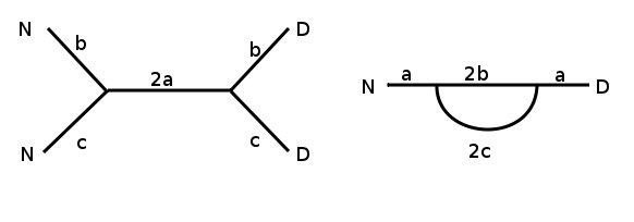
Figure 1: two isospectral quantum graphs

The $N$ and $D$ stand for Neumann and Dirichlet boundary conditions at the vertex, all inner vertices have Kirchhoff-Neumann boundary conditions. The numbers $a,b,c$ are positive real numbers that correspond to the edge lengths. The quantum graph on the right has periodic orbits of length $2a$ while the one on the left does not.

The proper definition of length-spectrum assigns a weight to each periodic orbit that depends on the boundary conditions at the vertices.

Definition 2.11.

The length-spectrum of a quantum graph is the list of lengths of periodic orbits, each weighted with the factor

$$A_{G}(l):=\sum_{p\in PO:{}l_{p}=l}2Re(\mathcal{A}_{p})$$ (15)

where the coefficient $\mathcal{A}_{p}$ is from the trace formula, equation 14. If there are no periodic orbits of length $l$ we set $A_{G}(l)=0$.

If two quantum graphs have the same length-spectrum we say they are length-isospectral.

Remark 2.12.

Note that in the above definition the weight of a single periodic orbit and thus the weight at a particular length can be negative. The graph on the right in figure 1 has two periodic orbits of length $2a$ but their weights sum to zero, the two graphs are length-isospectral.

Corollary 2.13 (Huber’s theorem).

The length-spectrum and the eigenvalue-spectrum (without the eigenvalue zero) of a quantum graph determine each other.

In particular, Laplace-isospectrality implies length-isospectrality and vice versa.

Proof.

This follows directly from the trace formula, equation 13. ∎

3 The eigenvalue-spectrum

Corollary 3.1.

We can rewrite the trace formula as follows.

$$\sum_{k\in\mathbb{R}_{>0}}m_{G}(k)\varphi(k)= \mathcal{L}\widehat{\varphi}(0)-\frac{1}{2}N\varphi(0)+\sum_{l\in\mathbb{R}_{>0}}A_{G}(l)\widehat{\varphi}(l)$$ (16)

Note that $m_{G}(k)$ and $A_{G}(l)$ are nonzero on a discrete set, so if $\varphi$ is a test function both sides of the equation converge absolutely.

Remark 3.2.

Notice that the multiplicity of the eigenvalue zero appears on both sides off the trace formula and cancels out.

Consider the unit interval with either Dirichlet or Neumann boundary conditions at both ends. Then these two quantum graphs have the same length-spectrum and the same eigenvalue-spectrum except the eigenvalue zero, which has multiplicity one for Neumann boundary conditions and multiplicity zero for Dirichlet boundary conditions.

This is an example of a more general phenomenon. Pick a quantum graph $G$ and create a new graph $G^{\prime}$ by switching the roles of the matrices $A$ and $B$ in the boundary conditions. Then $S^{\prime}=\overline{S}$ so these graphs have the same length-spectrum. Differentiating maps the eigenfunctions of one to the eigenfunctions of the other, thus $G$ and $G^{\prime}$ have the same eigenvalue-spectrum away from zero. However, the multiplicity of the eigenvalue zero does not have to agree in general.

Remark 3.3.

We have

$$\frac{1}{K}\sum_{k\in[0,K]}m_{G}(k)\sim\frac{\mathcal{L}}{\pi}$$ (17)

as $K\rightarrow\infty$ because $G$ has approximately $\frac{\mathcal{L}K}{\pi}$ eigenvalues in the interval $[0,K]$ by the Weyl law, theorem 2.7.

Theorem 3.4.

Let $G$ and $G^{\prime}$ be two quantum graphs with non-Robin type boundary conditions at all vertices. If

$$\lim_{K\rightarrow\infty}\frac{1}{K}\sum_{k\in[0,K]}\left|m_{G}(k)-m_{G^{\prime}}(k)\right|=0$$ (18)

then $G$ and $G^{\prime}$ are Laplace-isospectral (with the possible exception of the multiplicity of the eigenvalue zero) and length-isospectral. Here $m_{G}(k)$ is the multiplicity of the eigenvalue $k^{2}$ of $G$.

Proof.

If the limit above is zero, then $G$ and $G^{\prime}$ have the same eigenvalue asymptotics, so by the Weyl law, theorem 2.7, we have $\mathcal{L}=\mathcal{L}^{\prime}$.

Let $\psi\in C_{c}^{\infty}(\mathbb{R})$ such that $\operatorname{supp}(\psi)\subset[-1,1]$, $\psi(0)=1$ and $\psi$ is even. Fix $l_{0}\in\mathbb{R}$. Let

$$\psi_{K}(l):=\psi(K(l-l_{0}))+\psi(K(l+l_{0}))$$ (19)

for $K$ a large parameter (the idea to consider this kind of test function is adapted from [Kel11]). Then $\check{\psi}_{K}(k)=2\pi\widehat{\psi_{K}}(k)$ because $\psi_{K}$ is even. By the Paley-Wiener theorem (theorem 2.6), $\widehat{\psi_{K}}$ is holomorphic and rapidly decreasing. Thus $\check{\psi}_{K}$ is a valid test function (see definition 2.5) for the trace formula. We have $\check{\psi}_{K}(k)=\frac{4\pi}{K}\widehat{\psi}(\frac{k}{K})\cos(kl_{0})$. We plug $\check{\psi}_{K}$ in the difference of the trace formulas (corollary 3.1) for $G$ and $G^{\prime}$ and obtain

$$\left.\begin{split}&\frac{4\pi}{K}\sum_{k\in\mathbb{R}_{>0}}\left(m_{G}(k)-m_{G^{\prime}}(k)\right)\widehat{\psi}(\frac{k}{K})\cos(kl_{0})\\ =&-\frac{1}{2}(N-N^{\prime})\frac{4\pi}{K}\widehat{\psi}(0)+\sum_{l\in\mathbb{R}_{>0}}\left(A_{G}(l)-A_{G^{\prime}}(l)\right)\psi_{K}(l)\end{split}\right.$$ (20)

As $\widehat{\psi}$ is rapidly decreasing there exists a constant $C$ such that $\left|\widehat{\psi}(x)\right|<\frac{C}{(1+|x|)^{3}}$. We can bound

$$\left|\frac{4\pi}{K}\sum_{k\in\mathbb{R}_{\geqslant 0}}\left(m_{G}(k)-m_{G^{\prime}}(k)\right)\widehat{\psi}(\frac{k}{K})\cos(kl_{0})\right|$$ (21)

$$< \frac{4\pi}{K}\sum_{j=0}^{\infty}\sum_{k\in[jK,(j+1)K]}\left|m_{G}(k)-m_{G^{\prime}}(k)\right|\cdot\frac{C}{(1+(\frac{k}{K})^{3}}$$ (22)

$$< 4C\pi\sum_{j=0}^{\infty}\sum_{k\in[jK,(j+1)K]}\frac{1}{K}\left|m_{G}(k)-m_{G^{\prime}}(k)\right|\cdot\frac{1}{(1+j)^{3}}$$ (23)

$$\leqslant 4C\pi\sum_{j=0}^{\infty}\frac{1}{(j+1)^{2}}\sum_{k\in[0,(j+1)K]}\frac{\left|m_{G}(k)-m_{G^{\prime}}(k)\right|}{(j+1)K}$$ (24)

$$\leqslant 4C\pi\sum_{j=0}^{\infty}\frac{1}{(j+1)^{2}}\sup_{K^{\prime}\geqslant K}\sum_{k\in[0,K^{\prime}]}\frac{\left|m_{G}(k)-m_{G^{\prime}}(k)\right|}{K^{\prime}}$$ (25)

$$< 4C\pi\frac{\pi^{2}}{6}\sup_{K^{\prime}\geqslant K}\sum_{k\in[0,K^{\prime}]}\frac{\left|m_{G}(k)-m_{G^{\prime}}(k)\right|}{K^{\prime}}$$ (26)

$$\rightarrow 0$$ (27)

for $K\rightarrow\infty$ by the initial assumption.

For $K$ sufficiently large we have

$$\sum_{l\in\mathbb{R}_{>0}}\left(A_{G}(l)-A_{G^{\prime}}(l)\right)\psi_{K}(l)$$ (28)

$$= \left(A(l_{0},G)-A(l_{0},G^{\prime})\right)\psi_{K}(l_{0})$$ (29)

$$= \left(A(l_{0},G)-A(l_{0},G^{\prime})\right)$$ (30)

because the $l$ with $A_{G}(l)\neq 0$ are discrete and $\psi_{K}$ is supported around $l_{0}$ and $-l_{0}$. As all other terms in equation (20) go to zero for $K\rightarrow\infty$ this implies $A(l_{0},G)=A(l_{0},G^{\prime})$ for all $l_{0}$. Thus we have shown that $G$ and $G^{\prime}$ are length-isospectral. If we look at the difference of the trace formulae (20) and simplify we get

$$\sum_{k\in\mathbb{R}_{>0}}\left(m_{G}(k)-m_{G^{\prime}}(k)\right)\varphi(k)=-\frac{1}{2}(N-N^{\prime})\varphi(0)$$ (31)

By looking at a test function supported in a small enough neighborhood around $k$ we see that $m_{G}(k)=m_{G^{\prime}}(k)$ for all $k\neq 0$ and $N=N^{\prime}$ thus $G$ and $G^{\prime}$ are Laplace-isospectral, with the possible exception of the eigenvalue zero.

∎

The following example shows that our bound on the exceptional set is best possible.

Example 1.

Fix a value for $n$ and consider the following two quantum graphs, all edges have length one, all vertices have Kirchhoff-Neumann boundary conditions.

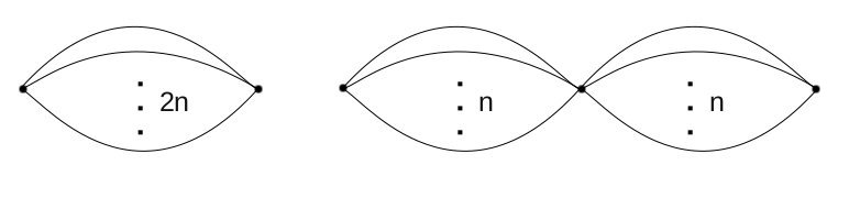
Figure 2: two quantum graphs whose spectra differ by a small proportion

Both quantum graphs are connected so $0$ is an eigenvalue with multiplicity one in both of them.

Let $k\in\mathbb{N}_{>0}$, then $k^{2}\pi^{2}$ is an eigenvalue of multiplicity $2n$ for the quantum graph on the left side. Assume all edges are parametrized from left to right as the interval $[0,1]$. Then there is one eigenfunction of the form $\cos(\pi kx)$ on all edges and a $(2n-1)$ dimensional eigenspace of functions of the form $a_{e}\sin(\pi kx)$ on each edge where the weights $a_{e}$ sum to zero.

For the quantum graph on the right again assume that all edges are parametrized from left to right as the interval $[0,1]$ and $k\in\mathbb{N}_{>0}$. There is one eigenfunction of the form $\cos(\pi kx/2)$ on the edges on the left and $\cos(\pi kx/2+1/2)$ on the edges on the right. There is a $(2n-2)$ dimensional eigenspace with eigenfunctions of the form $a_{e}\sin(\pi kx)$ on all edges where the sum of the $a_{e}$ over all edges on the right is zero and the sum over the $a_{e}$ over all edges on the left is zero. Thus the eigenvalues are the numbers $k^{2}\pi^{2}$ for $k\in\mathbb{N}_{>0}$ with multiplicity $2n-1$ union the numbers $k^{2}\pi^{2}/4$ for $k$ an odd positive integer.

This means these two quantum graphs satisfy

$$\lim_{K\rightarrow\infty}\frac{1}{K}\sum_{k\in[0,K]}|m_{G}(k)-m_{G^{\prime}}(k)|=\frac{2}{n}$$ (32)

which can be made arbitrarily small by choosing $n$ big enough.

4 The length-spectrum

Theorem 4.1.

Let $G$ and $G^{\prime}$ be quantum graphs with non-Robin type boundary conditions at all vertices. If

$$\lim_{L\rightarrow\infty}\frac{1}{L}\sum_{l\in[0,L]}|A_{G}(l)-A_{G^{\prime}}(l)|=0$$ (33)

then $G$ and $G^{\prime}$ are Laplace-isospectral (with the possible exception of the multiplicity of the eigenvalue zero) and length-isospectral.

Proof.

Let $\psi\in C_{c}^{\infty}(\mathbb{R})$ such that $\operatorname{supp}(\psi)\subset[-1,1]$, $\psi(0)=1$, $0\leqslant\psi(l)\leqslant 1$ and $\psi$ is even. Fix $k_{0}\in\mathbb{R}$. Let

$$\psi_{L}(l):=\frac{2}{L}\psi(\frac{l}{L})\cos(lk_{0})$$ (34)

for $L$ a large parameter. Then $\check{\psi_{L}}(k)=2\pi\widehat{\psi}(L(k-k_{0}))+2\pi\widehat{\psi}(L(k+k_{0}))$.

By the Paley-Wiener theorem (theorem 2.6), $\check{\psi}_{L}$ is a valid test function (see definition 2.5) for the trace formula. We plug $\check{\psi}_{L}$ in the difference of the trace formulas (corollary 3.1) for $G$ and $G^{\prime}$ and obtain

$$\left.\begin{split}&2\pi\sum_{k\in\mathbb{R}_{>0}}\left(m_{G}(k)-m_{G^{\prime}}(k)\right)\widehat{\psi_{L}}(k)\\ =&(\mathcal{L}-\mathcal{L}^{\prime})\psi_{L}(0)-\pi\left(N-N^{\prime}\right)\widehat{\psi_{L}}(0)+\sum_{l\in\mathbb{R}_{>0}}\left(A_{G}(l)-A_{G^{\prime}}(l)\right)\psi_{L}(l)\end{split}\right.$$ (35)

For the term involving the length-spectrum we can estimate

$$\left|\sum_{l\in\mathbb{R}_{>0}}\left(A_{G}(l)-A_{G^{\prime}}(l)\right)\psi_{L}(l)\right|$$ (36)

$$= \left|\sum_{l\in\mathbb{R}_{>0}}\left(A_{G}(l)-A_{G^{\prime}}(l)\right)\frac{2}{L}\psi(\frac{l}{L})\cos(lk_{0})\right|$$ (37)

$$\leqslant 2\left|\sum_{l\in[0,L]}\frac{A_{G}(l)-A_{G^{\prime}}(l)}{L}\right|$$ (38)

$$\rightarrow 0$$ (39)

as $L$ goes to infinity. We have $\psi_{L}(0)=\frac{2}{L}\rightarrow 0$ as $L$ goes to infinity. Similarly $\widehat{\psi_{L}}(0)=\widehat{\psi}(k_{0}L)+\widehat{\psi}(-k_{0}L)\rightarrow 0$ as $L$ goes to infinity because $\widehat{\psi}$ is rapidly decreasing.

This means we have

$$\lim_{L\rightarrow\infty}\sum_{k\in\mathbb{R}_{>0}}\left(m_{G}(k)-m_{G^{\prime}}(k)\right)\widehat{\psi_{L}}(k)=0$$ (40)

because all other terms in equation (35) go to zero in the limit $L\rightarrow\infty$. We have $\widehat{\psi_{L}}(k_{0})\rightarrow 2\pi\widehat{\psi}(0)\neq 0$ and $\widehat{\psi_{L}}(k)\rightarrow 0$ for all fixed $k\neq\pm k_{0}$ as $L\rightarrow\infty$. This implies $m_{G}(k_{0})=m_{G^{\prime}}(k_{0})$ for all $k_{0}>0$. Thus $G$ and $G^{\prime}$ have the same eigenvalue-spectrum with the possible exception of the eigenvalue zero, so by theorem 3.4 they are Laplace-isospectral and length-isospectral. ∎

Remark 4.2.

Note that $\sum_{l\in[0,L]}A_{G}(l)$ grows exponentially in $L$ so presumably our bound is not best possible.

5 Acknowledgement

This work was supported by a grant from EPSRC (grant EP/G021287/1).

References

- [BE08] Jens Bolte and Sebastian Endres, Trace formulae for quantum graphs, Analysis on graphs and its applications, Proc. Sympos. Pure Math., vol. 77, Amer. Math. Soc., Providence, RI, 2008, pp. 247–259.
- [BE09] , The trace formula for quantum graphs with general self adjoint boundary conditions, Ann. Henri Poincaré 10 (2009), no. 1, 189–223.
- [BPBS09] Ram Band, Ori Parzanchevski, and Gilad Ben-Shach, The isospectral fruits of representation theory: quantum graphs and drums, J. Phys. A 42 (2009), no. 17, 175202, 42.
- [BR11] Chandrasheel Bhagwat and C. S. Rajan, On a spectral analog of the strong multiplicity one theorem, Int. Math. Res. Not. IMRN (2011), no. 18, 4059–4073.
- [BSS06] Ram Band, Talia Shapira, and Uzy Smilansky, Nodal domains on isospectral quantum graphs: the resolution of isospectrality?, J. Phys. A 39 (2006), no. 45, 13999–14014.
- [DG75] J. J. Duistermaat and V. W. Guillemin, The spectrum of positive elliptic operators and periodic bicharacteristics, Invent. Math. 29 (1975), no. 1, 39–79.
- [EGM98] J. Elstrodt, F. Grunewald, and J. Mennicke, Groups acting on hyperbolic space, Springer Monographs in Mathematics, Springer-Verlag, Berlin, 1998, Harmonic analysis and number theory.
- [Gan77] Ramesh Gangolli, The length spectra of some compact manifolds of negative curvature, J. Differential Geom. 12 (1977), no. 3, 403–424.
- [Gri07] Daniel Grieser, Monotone unitary families, http://arxiv.org/abs/0711.2869 (2007).
- [GS01] Boris Gutkin and Uzy Smilansky, Can one hear the shape of a graph?, J. Phys. A 34 (2001), no. 31, 6061–6068.
- [GS06] Sven Gnutzmann and Uzy Smilansky, Quantum graphs: Applications to quantum chaos and universal spectral statistics, Advances in Physics 55 (2006), 527–625.
- [GW99] C. Gasquet and P. Witomski, Fourier analysis and applications, Texts in Applied Mathematics, vol. 30, Springer-Verlag, New York, 1999, Filtering, numerical computation, wavelets, Translated from the French and with a preface by R. Ryan.
- [Hör76] Lars Hörmander, Linear partial differential operators, Springer Verlag, Berlin, 1976.
- [Hub59] Heinz Huber, Zur analytischen Theorie hyperbolischen Raumformen und Bewegungsgruppen, Math. Ann. 138 (1959), 1–26.
- [Kel11] Dubi Kelmer, A refinement of strong multiplicity one for spectra of hyperbolic manifolds, http://arxiv.org/abs/1108.2977 (2011).
- [KPS07] Vadim Kostrykin, Jürgen Potthoff, and Robert Schrader, Heat kernels on metric graphs and a trace formula, Adventures in mathematical physics, Contemp. Math., vol. 447, Amer. Math. Soc., Providence, RI, 2007, pp. 175–198.
- [KS99] Tsampikos Kottos and Uzy Smilansky, Periodic orbit theory and spectral statistics for quantum graphs, Ann. Physics 274 (1999), no. 1, 76–124.
- [KS03] Vadim Kostrykin and Robert Schrader, Quantum wires with magnetic fluxes, Comm. Math. Phys. 237 (2003), no. 1-2, 161–179, Dedicated to Rudolf Haag. MR 2007178 (2005b:81047)
- [KS06] , Laplacians on metric graphs: eigenvalues, resolvents and semigroups, Quantum graphs and their applications, Contemp. Math., vol. 415, Amer. Math. Soc., Providence, RI, 2006, pp. 201–225.
- [Rot84] Jean-Pierre Roth, Le spectre du laplacien sur un graphe, Théorie du potentiel (Orsay, 1983), Lecture Notes in Math., vol. 1096, Springer, Berlin, 1984, pp. 521–539.
- [vB01] Joachim von Below, Can one hear the shape of a network?, Partial differential equations on multistructures (Luminy, 1999), Lecture Notes in Pure and Appl. Math., vol. 219, Dekker, New York, 2001, pp. 19–36.