Using blinking fractals for mathematical modeling of processes of growth in biological systems

Abstract

Many biological processes and objects can be described by fractals. The paper uses a new type of objects – blinking fractals – that are not covered by traditional theories considering dynamics of self-similarity processes. It is shown that both traditional and blinking fractals can be successfully studied by a recent approach allowing one to work numerically with infinite and infinitesimal numbers. It is shown that blinking fractals can be applied for modeling complex processes of growth of biological systems including their season changes. The new approach allows one to give various quantitative characteristics of the obtained blinking fractals models of biological systems.

Key Words: Process of growth, mathematical modeling in biology, traditional and blinking fractals, infinite and infinitesimal numbers.

1 Introduction

Fractals have been very well studied during the last few decades and have been used in various scientific fields including biology to model complex systems (see numerous applications given in [4, 5, 7, 12, 27]). The fractal objects are constructed by using the principle of self-similarity: a given basic figure (some times slightly modified in time) infinitely many times repeats itself in several copies. A simple example of such a construction is shown in Fig. 1. The basic figure shown in Step 1 is then repeated and already at Step 3 can be viewed as a simple model of a tree.

The introduction of fractals has allowed people to describe complex systems having a fractal structure in an elegant and very efficient way, to construct their computational models, and to study them. However, it is important to mention that mathematical analysis of fractals (except, of course, a very well developed theory of fractal dimensions, see [4, 5, 7, 12]) very often continues to have mainly a qualitative character. For example, tools for a quantitative analysis of fractals at infinity are not very rich yet (e.g., even for one of the mostly studied fractals – Cantor’s set – we are not able to count the number of intervals composing the set at infinity).

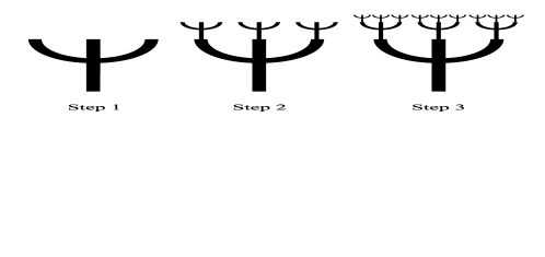
Figure 1: A simple fractal model of a tree.

Nowadays, fractals usually are used to describe objects (see, e.g., a tree presented in Fig. 1, Step 3) where one basic figure often called generator can be determined; they are rarely used for modeling processes where appearance of the studied objects is changed in time without preserving the generator. For example, the model from Fig. 1 cannot be used to describe a tree if we take into account season changes because in summer the tree has green leafs, in autumn the leafs are yellow, in winter there are no leafs at all and branches of the tree are under the snow. Thus, we are not able to distinguish one basic figure that maintains its form during the whole process and can be observed at all four seasons.

In nature, there exist processes and objects that evidently are very similar to classical fractals but cannot be covered by the traditional approaches because several self-similarity mechanisms participate in the process of their construction. A new methodology (see [15, 24]) allowing one not only to study traditional fractals but also to introduce and to investigate a new class of objects – blinking fractals – that are not covered by traditional theories studying self-similarity processes can be used for describing such processes.

The new methodology allowing one to work with such processes can be found in a rather comprehensive form in [18, 24] downloadable from [16] (see also the monograph [15] written in a popular manner and the survey [9] where the new methodology is considered in a historical panorama of views on infinities and infinitesimals). Numerous examples of the usage of the methodology [18, 24] for mathematical modelling in several fields can be found in [3, 10, 11, 14, 15, 17, 22, 20, 21, 23, 25, 26, 28, 29, 30]. The goal of the entire operation is to propose a way of thinking that would allow us to work with finite, infinite, and infinitesimal numbers in the same way and to create mathematical models better describing the natural phenomena.

In this paper, blinking fractals (see [17]) are used to model season changes and processes of growth in biological systems. The paper not only proposes such a modeling but also describes mathematical tools allowing one to study the properties of processes of growth in the limit even in the situations where various kinds of divergency take place.

The rest of the paper is organized as follows. Section 2 introduces the notion of blinking fractals, presents some examples, and briefly introduces the methodology used in the further investigation. In Section 3, it is shown how the blinking fractals can be investigated by using the infinite and infinitesimal numbers from [18, 24]. Section 4 shows how processes of growth of biological systems can be modelled by using the blinking fractals, particularly, the new applied approach to infinity is used to study a model of the growth of a forest. Section 5 concludes the paper.

In conclusion of the Introduction I am happy to dedicate this paper to Professor Jonas Mockus in the occasion of his 80 year jubilee.

2 Blinking fractals and infinite integers

Before going to a general definition of blinking fractals let us consider a process shown in Fig. 2. At the first moment we see a grey square with the side equal to 1. At the second moment we see two white circles with the diameter equal to $\frac{1}{2}$. Then each white circle is substituted by to grey squares $\frac{1}{2}$ on side. This process of substitution continues in time as it shown in Fig. 2.

It is clear that the process shown in Fig. 2 is not a fractal process because at each even iteration squares are not transformed in smaller copies of themselves but in circles (see Fig. 2 and Fig. 3, left). Analogously, at odd iterations circles are transformed in squares instead of smaller circles (see Fig. 2 and Fig. 3, right). Thus, the process shown in Fig. 2 is a mixture of two fractal processes with the rules shown in Fig. 4: the first of them works with grey squares and the second with white circles.

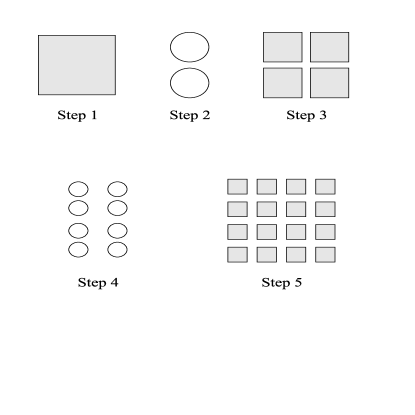
Figure 2: Results of the first five iterations.

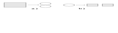
Figure 3: At each even iteration every square with a side equal to $h$ is substituted by two circles having the diameter $\frac{h}{2}$. At each odd iteration every circle with a diameter $d$ is substituted by two squares with $d$ on side.

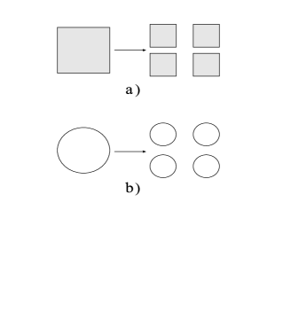
Figure 4: Two traditional fractal processes that can be extracted from the blinking fractal process shown in Fig. 2.

Traditional approaches are not able to say anything about the behavior of this process from Fig. 2 at infinity. Does there exist a limit object of this process? If it exists, what can we say about its structure? Does it consist of white circles or grey squares and how many of them take part of this limit object? All these questions remain without answers if traditional mathematical tools are used for analysis of such processes.

In this paper, we give answers to these questions by using a new approach developed in [15, 18, 24] for dealing with infinite, finite, and infinitesimal numbers. The new methodology will be applied to study traditional fractals and new objects constructed using the principle of self-similarity with an infinite cyclic application of several fractal rules. These objects are called hereinafter blinking fractals.

Usually, when mathematicians deal with infinite objects (sets or processes) it is supposed that human beings are able to execute certain operations infinitely many times (see [1, 2, 8, 13]). For example, in a fixed numeral system it is possible to write down a numeral with any number of digits. However, this supposition is an abstraction because we live in a finite world and all human beings and/or computers finish operations they have started.

The new computational paradigm introduced in [15, 18, 24] does not use this abstraction and, therefore, is closer to the world of practical calculations than traditional approaches. Its strong computational character is enforced also by the fact that the first simulator of the Infinity Computer able to work with infinite, finite, and infinitesimal numbers introduced in [15, 18, 24] has been already realized (see [16, 19]).

The main idea of the new approach consists of the possibility to measure infinite and infinitesimal quantities by different (infinite, finite, and infinitesimal) units of measure. A new infinite unit of measure has been introduced for this purpose as the number of elements of the set $\mathbb{N}$ of natural numbers. The new number is called grossone and is expressed by the numeral ①. It is necessary to stress immediately that ① is not related either to non-standard analysis or to Cantor’s $\aleph_{0}$ and $\omega$. Particularly, ① has both cardinal and ordinal properties as usual finite natural numbers (see [18, 23, 24]). In fact, infinite positive integers that can be viewed through numerals including grossone can be interpreted in the terms of the number of elements of certain infinite sets.

For instance, the set of even numbers has $\frac{\hbox{$\displaystyle{\mbox{\char 172}}$}}{2}$ elements and the set of integers has $2\mbox{\hbox{$\displaystyle{\mbox{\char 172}}$}\small{+}}1$ elements (see [18, 23, 24]). Thus, the new numeral system allows one to distinguish within countable sets many different sets having the different infinite number of elements. Analogously, within uncountable sets it is possible to distinguish sets having, for instance, $2^{\mbox{\tiny{\hbox{$\displaystyle{\mbox{\char 172}}$}}}}$ elements, $10^{\mbox{\tiny{\hbox{$\displaystyle{\mbox{\char 172}}$}}}}$ elements, and even $\hbox{$\displaystyle{\mbox{\char 172}}$}^{\mbox{\tiny{\hbox{$\displaystyle{\mbox{\char 172}}$}}}}-1$, $\hbox{$\displaystyle{\mbox{\char 172}}$}^{\mbox{\tiny{\hbox{$\displaystyle{\mbox{\char 172}}$}}}}$, and $\hbox{$\displaystyle{\mbox{\char 172}}$}^{\mbox{\tiny{\hbox{$\displaystyle{\mbox{\char 172}}$}}}}+1$ elements and to show (see [18, 23, 24]) that

$$\frac{\hbox{$\displaystyle{\mbox{\char 172}}$}}{2}<\hbox{$\displaystyle{\mbox{\char 172}}$}<2\mbox{\hbox{$\displaystyle{\mbox{\char 172}}$}\small{+}}1<2^{\mbox{\tiny{\hbox{$\displaystyle{\mbox{\char 172}}$}}}}<10^{\mbox{\tiny{\hbox{$\displaystyle{\mbox{\char 172}}$}}}}<\hbox{$\displaystyle{\mbox{\char 172}}$}^{\mbox{\tiny{\hbox{$\displaystyle{\mbox{\char 172}}$}}}}-1<\hbox{$\displaystyle{\mbox{\char 172}}$}^{\mbox{\tiny{\hbox{$\displaystyle{\mbox{\char 172}}$}}}}<\hbox{$\displaystyle{\mbox{\char 172}}$}^{\mbox{\tiny{\hbox{$\displaystyle{\mbox{\char 172}}$}}}}+1.$$

It is worthwhile to emphasize that since ①, on the one hand, and $\aleph_{0}$ (and $\omega$), on the other hand, belong to different mathematical languages working with different theoretical assumptions, they cannot be used together. Analogously, it is not possible to use together Piraha’s ‘many’ (see the primitive numeral system described in [6]) and the modern numeral 4.

Formally, grossone is introduced as a new number by describing its properties postulated by the Infinite Unit Axiom (IUA) (see [15, 18]). This axiom is added to axioms for real numbers similarly to addition of the axiom determining zero to axioms of natural numbers when integer numbers are introduced. It is important to emphasize that we speak about axioms for real numbers in the following applied sense: axioms do not define real numbers, they just define formal rules of operations with numerals in given numeral systems (tools of the observation) reflecting so certain (not all) properties of the object of the observation, i.e., properties of real numbers.

Inasmuch as it has been postulated that grossone is a number, all other axioms for numbers hold for it, too. Particularly, associative and commutative properties of multiplication and addition, distributive property of multiplication over addition, existence of inverse elements with respect to addition and multiplication hold for grossone as for finite numbers. This means that the following relations hold for grossone, as for any other number

$$0\cdot\hbox{$\displaystyle{\mbox{\char 172}}$}=\hbox{$\displaystyle{\mbox{\char 172}}$}\cdot 0=0,\hskip 8.53581pt\hbox{$\displaystyle{\mbox{\char 172}}$}-\hbox{$\displaystyle{\mbox{\char 172}}$}=0,\hskip 8.53581pt\frac{\hbox{$\displaystyle{\mbox{\char 172}}$}}{\hbox{$\displaystyle{\mbox{\char 172}}$}}=1,\hskip 8.53581pt\hbox{$\displaystyle{\mbox{\char 172}}$}^{0}=1,\hskip 8.53581pt1^{\mbox{\tiny{\hbox{$\displaystyle{\mbox{\char 172}}$}}}}=1,\hskip 8.53581pt0^{\mbox{\tiny{\hbox{$\displaystyle{\mbox{\char 172}}$}}}}=0.$$ (1)

The introduction of the new numeral allows us to use it for construction of various new numerals expressing infinite and infinitesimal numbers and to operate with them as with usual finite constants. As a consequence, the numeral $\infty$ is excluded from our new mathematical language (together with numerals $\aleph_{0},\aleph_{1},\ldots$ and $\omega$). In fact, since we are able now to express explicitly different infinite numbers, records of the type $\sum_{i=1}^{\infty}a_{i}$ are not sufficiently precise. It becomes necessary not only to say that $i$ goes to infinity, it is necessary to indicate to which point in infinity (e.g., $\hbox{$\displaystyle{\mbox{\char 172}}$},7\hbox{$\displaystyle{\mbox{\char 172}}$}-1,3\hbox{$\displaystyle{\mbox{\char 172}}$}^{2}+4$, etc.) we want to sum up. Note that for sums having a finite number of items the situation is the same: it is not sufficient to say that the number of items in the sum is finite, it is necessary to indicate explicitly the number of items in the sum.

The appearance of new numerals expressing infinite and infinitesimal numbers gives us a lot of new possibilities. For example, it becomes possible to develop a Differential Calculus (see [22]) for functions that can assume finite, infinite, and infinitesimal values and can be defined over finite, infinite, and infinitesimal domains avoiding indeterminate forms and divergences (all these concepts just do not appear in the new Calculus). This approach allows us to work with derivatives and integrals that can assume not only finite but infinite and infinitesimal values, as well. Infinite and infinitesimal numbers are not auxiliary entities in the new Calculus, they are full members in it and can be used in the same way as finite constants.

These numerals give us a possibility to study traditional fractals and blinking fractals at different points of infinity and to use them for modeling the nature. In this section, we investigate the blinking fractal introduced in Section 2 and infinite sequences will be used for this goal. Naturally, we need first to understand what can we say about the infinite sequences using the new mathematical language.

3 Quantitative analysis of blinking fractals

We start by reminding traditional definitions of the infinite sequences and subsequences. An infinite sequence $\{a_{n}\},a_{n}\in A,n\in\mathbb{N},$ is a function having as the domain the set of natural numbers, $\mathbb{N}$, and as the codomain a set $A$. A subsequence is a sequence from which some of its elements have been cancelled. The IUA allows us to prove the following result.

Theorem 1.

The number of elements of any infinite sequence is less or equal to ①.

Proof. The IUA states that the set $\mathbb{N}$ has ① elements. Thus, due to the sequence definition given above, any sequence having $\mathbb{N}$ as the domain has ① elements.

The notion of subsequence is introduced as a sequence from which some of its elements have been cancelled. Thus, this definition gives infinite sequences having the number of members less than grossone. $\Box$

It becomes appropriate now to define the complete sequence as an infinite sequence containing ① elements. For example, the sequence $\{n\}$ of natural numbers is complete, the sequences of even and odd natural numbers are not complete.

One of the immediate consequences of the understanding of this result is that any sequential process can have at maximum ① elements and (see [15, 18]) it depends on the chosen numeral system which numbers among ① members of the process we can observe.

Example 1.

Let us consider the set, $\widehat{\mathbb{N}}$, the set of extended natural numbers indicated as $\widehat{\mathbb{N}}$ and including $\mathbb{N}$ as a proper subset

$$\widehat{\mathbb{N}}=\{1,2,\ldots,\mbox{\char 172}-1,\mbox{\char 172},\mbox{\char 172}+1,\ldots,\mbox{\char 172}^{2}-1,\mbox{\char 172}^{2},\mbox{\char 172}^{2}+1,\ldots\}.$$ (2)

Then, starting from the number 1, the process of the sequential counting can arrive at maximum to ①

$$\underbrace{1,2,3,4,\hskip 2.84526pt\ldots\hskip 2.84526pt\mbox{\char 172}-2,\hskip 2.84526pt\mbox{\char 172}-1,\mbox{\char 172}}_{\mbox{\char 172}},\mbox{\char 172}+1,\mbox{\char 172}+2,\mbox{\char 172}+3,\ldots$$

Starting from 2 it arrives at maximum to $\mbox{\char 172}+1$

$$1,\underbrace{2,3,4,\hskip 2.84526pt\ldots\hskip 2.84526pt\mbox{\char 172}-2,\hskip 2.84526pt\mbox{\char 172}-1,\mbox{\char 172},\mbox{\char 172}+1}_{\mbox{\char 172}},\mbox{\char 172}+2,\mbox{\char 172}+3,\ldots$$

Starting from 3 it arrives at maximum to $\mbox{\char 172}+2$

                 $$1,2,\underbrace{3,4,\hskip 2.84526pt\ldots\hskip 2.84526pt\mbox{\char 172}-2,\hskip 2.84526pt\mbox{\char 172}-1,\mbox{\char 172},\mbox{\char 172}+1,\mbox{\char 172}+2}_{\mbox{\char 172}},\mbox{\char 172}+3,\ldots$$             

Similarly to infinite sets, the IUA imposes a more precise description of infinite sequences. To define a sequence $\{a_{n}\}$ it is not sufficient just to give a formula for $a_{n}$. It is necessary to indicate explicitly its number of elements.

Example 2.

Let us consider the following three sequences, $\{a_{n}\},\{b_{n}\},$ and $\{c_{n}\}$:

$$\{a_{n}\}=\{2,\hskip 8.53581pt4,\hskip 8.53581pt\ldots\hskip 8.53581pt2(\mbox{\char 172}-1),\hskip 8.53581pt2\mbox{\char 172}\},$$

$$\{b_{n}\}=\{2,\hskip 8.53581pt4,\hskip 8.53581pt\ldots\hskip 8.53581pt2(\frac{2\mbox{\char 172}}{5}-1),\hskip 8.53581pt2\cdot\frac{2\mbox{\char 172}}{5}\},$$ (3)

$$\{c_{n}\}=\{2,\hskip 8.53581pt4,\hskip 8.53581pt\ldots\hskip 8.53581pt2(\frac{4\mbox{\char 172}}{5}-1),\hskip 8.53581pt2\cdot\frac{4\mbox{\char 172}}{5}\}.$$ (4)

They have the same general element equal to $2n$ but they are different because they have different number of members. The first sequence has ① elements and is thus complete, the other two sequences are not complete: $\{b_{n}\}$ has $\frac{2\mbox{\char 172}}{5}$ elements and $\{c_{n}\}$ has $\frac{4\mbox{\char 172}}{5}$ members. Note also that among these three sequences only $\{b_{n}\}$ is a subsequence of the sequence of even natural numbers because its last element has the number $\frac{2\mbox{\char 172}}{5}\leq\frac{\mbox{\char 172}}{2}$. Since ① is the last even natural number, elements of $\{a_{n}\}$ and $\{c_{n}\}$ having $n>\frac{\mbox{\char 172}}{2}$ are not natural but extended natural numbers (see (2)). $\Box$

Thus, to describe a sequence we should use the record $\{a_{n}:k\}$ where $a_{n}$ is, as usual, the general element and $k$ is the number (finite or infinite) of members of the sequence. In connection to this definition the following natural question arises inevitably. Suppose that we have two sequences, for example, $\{b_{n}:\frac{2\mbox{\char 172}}{5}\}$ and $\{c_{n}:\frac{4\mbox{\char 172}}{5}\}$ from (3) and (4). Can we create a new sequence, $\{d_{n}:k\}$, composed from both of them, for instance, as it is shown below

$$b_{1},\hskip 2.84526ptb_{2},\hskip 2.84526pt\ldots\hskip 2.84526ptb_{\frac{2\mbox{\tiny{\char 172}}}{5}-2},\hskip 2.84526ptb_{\frac{2\mbox{\tiny{\char 172}}}{5}-1},\hskip 2.84526ptb_{\frac{2\mbox{\tiny{\char 172}}}{5}},\hskip 2.84526ptc_{1},\hskip 2.84526ptc_{2},\hskip 2.84526pt\ldots\hskip 2.84526ptc_{\frac{4\mbox{\tiny{\char 172}}}{5}-2},\hskip 2.84526ptc_{\frac{4\mbox{\tiny{\char 172}}}{5}-1},\hskip 2.84526ptc_{\frac{4\mbox{\tiny{\char 172}}}{5}}$$

and which will be the value of the number of its elements $k$?

The answer is ‘no’ because due to the definition of the infinite sequence, a sequence can be at maximum complete, i.e., it cannot have more than ① elements. Starting from the element $b_{1}$ we can arrive at maximum to the element $c_{\frac{3\mbox{\tiny{\char 172}}}{5}}$ being the element number ① in the sequence $\{d_{n}:k\}$ which we try to construct. Therefore, $k=\mbox{\char 172}$ and

$$\underbrace{b_{1},\hskip 2.84526pt\ldots\hskip 2.84526ptb_{\frac{2\mbox{\tiny{\char 172}}}{5}},\hskip 2.84526ptc_{1},\hskip 2.84526pt\ldots c_{\frac{3\mbox{\tiny{\char 172}}}{5}}}_{\mbox{\char 172 elements}},\hskip 2.84526pt\underbrace{c_{\frac{3\mbox{\tiny{\char 172}}}{5}+1},\ldots\hskip 2.84526ptc_{\frac{4\mbox{\tiny{\char 172}}}{5}}}_{\frac{\mbox{\tiny{\char 172}}}{5}\mbox{ elements }}.$$

The remaining members of the sequence $\{c_{n}:\frac{4\mbox{\char 172}}{5}\}$ will form the second sequence, $\{g_{n}:l\}$ having $l=\frac{4\mbox{\char 172}}{5}-\frac{3\mbox{\char 172}}{5}=\frac{\mbox{\char 172}}{5}$ elements. Thus, we have formed two sequences, the first of them is complete and the second is not.

The introduced more precise description of sequences allows us to observe fractal processes at different points of infinity by indicating the number of a step, $n,1\leq n\leq\mbox{\char 172},$ that we want to study. For example, for our blinking fractal from Fig. 2 we are able to say that we observe grey squares at all odd steps and white circles at even steps independently of the fact $n$ is finite or infinite. Particularly, since due to the Infinite Unit Axiom $\frac{\mbox{\char 172}}{2}$ is integer, for $n=\mbox{\char 172}$ we have white circles and for $n=\mbox{\char 172}-1$ – grey squares.

In order to be able to measure fractals at infinity (e.g., to calculate the number of squares or circles at a step $n$ in our blinking fractal from Fig. 2), we should reconsider the theory of divergent series from the new viewpoint introduced in the previous sections. The introduced numeral system allows us to express not only different finite numbers but also different infinite numbers. Therefore (see [15, 18]) we should explicitly indicate the number of items in all sums independently on the fact whether this number is finite or infinite. We shall be able to calculate the sum if its items, the number of items, and the result are expressible in the numeral system used for calculations. It is important to notice that even though a sequence cannot have more than ① elements, the number of items in a sum can be greater than grossone because the process of summing up not necessary should be executed by a sequential addition of items.

For instance, let us consider two infinite series

$$S_{1}=1+2+4+8+16+\ldots,\hskip 42.67912ptS_{2}=1+2+1+2+1+2+1\ldots$$

The traditional analysis gives us a very poor answer that both of them diverge to infinity. Such operations as $S_{1}-S_{2}$ or $\frac{S_{1}}{S_{2}}$ are not defined. From the new point of view, the sums $S_{1}$ and $S_{2}$ can be calculated because it is necessary to indicate explicitly the number of items in both sums.

Suppose that the sum $S_{1}$ has $m+1$ items and the sum $S_{2}$ has $n$ items:

$$S_{1}(m)=\underbrace{1+2+4+8+\ldots+2^{m}}_{m+1},\hskip 17.07164ptS_{2}(n)=\underbrace{1+2+1+2+1+\ldots}_{n}.$$ (5)

Let us first calculate the sum $S_{1}(m)$. It is evident that it is a particular case of the sum

$$Q_{m}=\sum_{i=0}^{m}q^{i}=1+q+q^{2}+\ldots+q^{m},$$ (6)

where $m$ can be finite or infinite. Traditional analysis proves that the geometric series $\sum_{i=0}^{\infty}q^{i}$ converges to $\frac{1}{1-q}$ for $q$ such that $-1<q<1$. We are able to give a more precise answer for all values of $q$ and finite and infinite values of $m$.

By multiplying the left hand and the right hand parts of this equality by $q$ and by subtracting the result from (6) we obtain

$$Q_{m}-qQ_{m}=1-q^{m+1}$$

and, as a consequence, for all $q\neq 1$ the formula

$$Q_{m}=\frac{1-q^{m+1}}{1-q}$$ (7)

holds for finite and infinite $m$. Thus, the possibility to express infinite and infinitesimal numbers allows us to take into account infinite $m$ too and the value $q^{m+1}$ being infinitesimal for a finite $q<1$ and infinite for $q>1$. Moreover, we can calculate $Q_{m}$ for $q=1$. In fact, in this case we have just

$$Q_{m}=\underbrace{1+1+1+\ldots+1}_{m+1}=m+1.$$

Now, to calculate the sum $S_{1}(m)$ it is sufficient to take $q=2$

$$S_{1}(m)=\underbrace{1+2+4+8+16+\ldots+2^{m}}_{m+1}=\frac{1-2^{m+1}}{1-2}=2^{m+1}-1.$$

This formula can be used for finite and infinite values of $m$. For instance, if $m=\frac{\mbox{\char 172}}{2}-1$ then $S_{1}(\frac{\mbox{\char 172}}{2}-1)=2^{\frac{\mbox{\tiny{\char 172}}}{2}}-1$; if $m=\frac{\mbox{\char 172}}{2}$ then $S_{1}(\frac{\mbox{\char 172}}{2})=2^{\frac{\mbox{\tiny{\char 172}}}{2}+1}-1$. Note that the sum $S_{1}(\frac{\mbox{\char 172}}{2})$ has been obtained by adding $2^{\frac{\mbox{\tiny{\char 172}}}{2}}$ to the sum $S_{1}(\frac{\mbox{\char 172}}{2}-1)$. In fact, if we subtract from the obtained number $2^{\frac{\mbox{\tiny{\char 172}}}{2}+1}-1$ this value, we obtain exactly $S_{1}(\frac{\mbox{\char 172}}{2}-1)$:

$$S_{1}(\frac{\mbox{\char 172}}{2})-2^{\frac{\mbox{\tiny{\char 172}}}{2}}=2^{\frac{\mbox{\tiny{\char 172}}}{2}+1}-1-2^{\frac{\mbox{\tiny{\char 172}}}{2}}=2^{\frac{\mbox{\tiny{\char 172}}}{2}}-1=S_{1}(\frac{\mbox{\char 172}}{2}-1).$$

The second sum, $S_{2}(n)$, from (5) is calculated as follows

$$S_{2}(n)=\underbrace{1+2+1+2+1+\ldots}_{n}=\left\{\begin{array}[]{ll}k+2k=3k,&\mbox{if }n=2k,\\ k+2k+1=3k+1,&\mbox{if }n=2k+1.\\ \end{array}\right.$$

By giving numerical values (finite or infinite) to $n$ we obtain numerical values for results of the sum. If, for instance, $n=3\mbox{\char 172}$ then we obtain $S_{2}(3\mbox{\char 172})=4.5\mbox{\char 172}$ because ① is even. If $n=3\mbox{\char 172}+1$ then we obtain $S_{2}(3\mbox{\char 172}+1)=4.5\mbox{\char 172}+1$. Note, that we have no indeterminate expressions and the results such as $S_{2}(m)-S_{2}(n),$ $S_{1}(m)-S_{2}(n),$ $\frac{S_{2}(m)}{S_{2}(n)},$ etc. can be easily calculated.

Let us now return to fractals. First of all, it is evident that the number of circles or squares at a step $i,1\leq i\leq\mbox{\char 172}$, in the blinking process from Fig. 2 is defined by the sum $S_{1}(i-1)$. It is important to remind that, due to the IUA, a process cannot have more than grossone steps but a sum can have more than grossone items because it can be calculated in parallel (it is important that it is not calculated in sequence). Thus, if we consider the process from Fig. 2, then in $S_{1}(i)$ it follows $1\leq i\leq\mbox{\char 172}$. It is possible to calculate $S_{1}(i),i>\mbox{\char 172},$ if this is done without any connection to processes (i.e., $S_{1}(i)$ can be computed in parallel) or in connection with another process with other different initial conditions. For instance, starting the process from Fig. 2 from two circles instead of one square, it is possible to arrive to $S_{1}(\mbox{\char 172}+1),$ see discussion in Example 1).

We conclude this section by calculating the side of the squares, $s(i),i=2k-1,1\leq k\leq\frac{\mbox{\char 172}}{2}$, and the diameter of circles, $d(i),i=2k,1\leq k\leq\frac{\mbox{\char 172}}{2}$, for the blinking fractal from Fig. 2. It is easily to show that

$$s(i)=\frac{1}{2^{k-1}},\hskip 28.45274pti=2k-1,\hskip 14.22636pt1\leq k\leq\frac{\mbox{\char 172}}{2},$$

$$d(i)=\frac{1}{2^{k}},\hskip 28.45274pti=2k,\hskip 14.22636pt1\leq k\leq\frac{\mbox{\char 172}}{2}.$$

For finite values of $i$ we obtain finite values of $s(i)$ and $d(i)$, whereas for infinite values of $i$ we obtain infinitesimal values of $s(i)$ and $d(i)$. For example, for $i=\frac{\mbox{\char 172}}{3}$ it follows that we have white circles (because due to the IUA, for all finite integer $n$ the numbers of the form $\frac{\mbox{\char 172}}{n}$ are integer and, therefore, $i=\frac{\mbox{\char 172}}{3}$ is even) and their diameter $d(\frac{\mbox{\char 172}}{3})=2^{-\frac{\mbox{\tiny{\char 172}}}{6}}$. Analogously, for $i=\frac{\mbox{\char 172}}{3}-1$ we have grey squares having the side $s(\frac{\mbox{\char 172}}{3}-1)=2^{1-\frac{\mbox{\tiny{\char 172}}}{6}}$.

Thus, the new infinite and infinitesimal numerals allow us to observe and to measure the traditional and blinking fractals at different points of infinity.

4 A blinking fractals model of the growth of a forest and its analysis at infinity

Figure 5: The first year of growth.

The analysis performed in the previous section allows us to pass to modeling processes in nature having a blinking fractals structure. Without loss of the generality we consider biennial plants (called hereinafter for simplicity trees) that will be observed four times a year: in spring, in summer, in autumn, and in winter. The process of growth starts in spring by planting two small trees (see Fig. 5, spring) in a line. In summer, the trees grow up and green leafs (shown by grey color) appear. During summer new branches appear and when we observe our trees in autumn, we see these new branches and leafs that meanwhile have became yellow (shown in Fig. 5 by the light grey color). When we observe our small forest in winter, there are no leafs and the trees are under the snow.

Figure 6: The second year of growth.

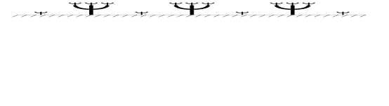
Figure 7: Spring of the third year of growth.

When we observe our forest in spring of the second year (see Fig. 6, spring), we see that three new trees have appeared (we suppose that the growth goes along the line defined by the first two trees). In summer of the second year, we see green leafs and observe that the new trees have grown up but the old two trees are not able to grow up and remain the same. In autumn, all five trees have the same measure and yellow leafs. In winter, all of them are under the snow. During the winter two old trees die and at their places new young trees appear. Two more new trees appear also at the free places on the left and the right ends of our forest. Thus, in spring of the third year we observe the situation shown in Fig. 7.

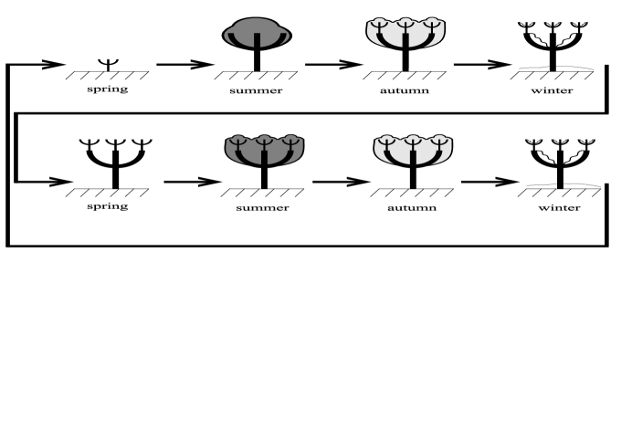
Figure 8: The two years cycle of growth.

The process then continues to infinity and at each place where a tree appears we can observe the two years cycle shown in Fig. 8. It is evident that the described model is not a fractal. By using traditional mathematics we are not able to answer to the following questions: How many trees and how many branches will have our forest at infinity? What will be color of the leafs? However, we can separate from the process of growth several processes behaving as fractals and, as a consequence, the process of growth of our forest is a blinking fractal. The new approach introduced in the previous section will allow us to give quantitative answers to the questions above easily.

Figure 9: The winter process.

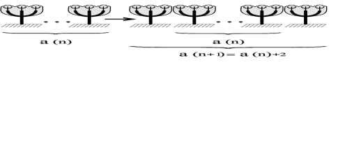
Figure 10: The autumn process.

It is evident that during each season we have different basic figures and it is necessary to consider the forest at each season separately by applying the methodology of blinking fractals. Let us start from winter. If $n$ is the number of the year then (see Fig. 9) we can easily calculate the number of trees at the forest, $\omega(n)$, for each year $n$ as follows

$$\omega(1)=2,\,\,\,\,\omega(2)=5,\,\,\,\,\omega(3)=7,\ldots\,\,\,\,\omega(n)=2n+1,\,\,\,\,n\geq 2.$$

An analogous formula for calculating the number of the trees in autumn, $a(n)$, can be obtained (see Fig. 10) for the autumn process

$$a(1)=2,\,\,\,\,a(2)=5,\,\,\,\,a(3)=7,\ldots\,\,\,\,a(n)=2n+1,\,\,\,\,n\geq 2.$$

The same formulae for calculating the number of trees can be obtained for spring and summer, because the number of trees is the same during four seasons of each fixed year. Note that since we observe our forest four time per year and any process, due to the IUA, cannot have more than ① elements, the following restriction exists for the number, $n$, of the years of observations of our forest: $1\leq n\leq\frac{\mbox{\char 172}}{4}$. This means, particularly, that the number of the trees at the last year $a(\frac{\mbox{\char 172}}{4})=\frac{\mbox{\char 172}}{2}+1$.

Figure 11: Two summer processes.

Figure 12: Two spring processes.

Although the number of the trees does not change during each fixed year, the changes take place for the number of branches; the form of the basic figures is also different for each season. Moreover, as it emphasized in Figs. 11 and 12, the processes in summer and spring are more complex than the processes in winter and autumn because we can distinguish the processes of growth of the same tree (parts a) in both figures) and the process of substitution of an old tree by the young one (shown in parts b) in both figures). For these two seasons we are able to calculate the number of old trees, the number of young trees, and even the number of branches in the forest for each of four seasons.

Let us first calculate the number of young and old trees in summer indicated as $y(i)$ and $o(i)$, respectively, that there are in the forest during an observation $i$ made in the year $n$ (as it can be seen from Figs. 5 and 6, in spring we have the same quantities that can be calculated by a complete analogy). Since it can be done at maximum grossone observations, it follows from description of the process of the growth that for years $n=1,2,3,\,\,\ldots,\frac{\mbox{\char 172}}{4},$ the numbers of observations corresponding to summer are $i=2,6,10,\,\,\ldots,\,\,2+4(n-1),\ldots,\mbox{\char 172}-2$. Thus, the numbers of young and old trees in summer are calculated as follows

$$y(2+4(n-1))=n+1,\hskip 28.45274pt1\leq n\leq\frac{\mbox{\char 172}}{4},$$ (8)

$$o(2)=0,\hskip 14.22636pto(2+4(n-1))=n,\hskip 28.45274pt2\leq n\leq\frac{\mbox{\char 172}}{4}.$$ (9)

Let us calculate now the number of the branches in the forest for each season. We indicate this number as $b(i)$ where $i$ is the number of observation. In winter, all the trees have the same number of branches: three big and nine small. The observations $i=4n$ correspond to winter at the year $n$ and there are $2n+1$ trees in the forest. Thus, we obtain $b(4n)=12(2n+1)$. Analogously, the observations $i=3+4(n-1)$ correspond to autumn at the year $n$ and, consequently, the number of branches in autumn $b(3+4(n-1))=12(2n+1)$ as well.

In spring and summer, the situation is different: young and old trees have different number of branches (see Figs. 5,6,11, and 12). Let us consider summer (spring can be studied by a complete analogy). In summer young trees have three big branches each and old trees have 12 branches each: three big and nine small.

Remind, that the observations at the year $n$ corresponding to summer have numbers $i=2+4(n-1)$. Thus, in order to obtain the required result it is sufficient to use formulae (8) and (9) that give us

$$b(2)=6,\hskip 14.22636ptb(2+4(n-1))=3(n+1)+9n=12n+3,\hskip 28.45274pt2\leq n\leq\frac{\mbox{\char 172}}{4}.$$

For example, in summer of the last possible year of observation, $n=\frac{\mbox{\char 172}}{4}$, our forest has $3\mbox{\char 172}+3$ branches.

5 Concluding remarks

Fractals have been widely used in literature to model complex systems. In this paper, a new type of objects – blinking fractals – that are not covered by traditional theories studying self-similarity processes have been used for studying season changes during the growth of biological systems. The behavior of blinking fractals at infinity has been investigated using infinite and infinitesimal numbers proposed recently and a number of quantitative characteristics has been obtained.

As an example of application of the developed mathematical tools for describing the behavior of complex biological systems a new model of growth of a forest has been introduced and investigated using the notion of the blinking fractals. The new mathematical tools introduced in the paper have allowed us to separate in this complex model several fractal processes and to perform their accurate quantitative analysis. It is evident that the introduced model can be easily generalized to describe more complex objects and systems. For example, it is possible to introduce plants with the cycle of life superior to two years, the plants having a more complex structure can be also described by the introduced approach. In the future it is possible also to study some additional mechanisms (for instance, plant pests or nature disasters) that influence the process of growth.

References

- [1] G. Cantor. Contributions to the founding of the theory of transfinite numbers. Dover Publications, New York, 1955.
- [2] J.H. Conway and R.K. Guy. The Book of Numbers. Springer-Verlag, New York, 1996.
- [3] S. De Cosmis and R. De Leone. The use of grossone in mathematical programming and operations research. Applied Mathematics and Computation, (to appear).
- [4] R.L. Devaney. An Introduction to Chaotic Dynamical Systems. Westview Press Inc., New York, 2003.
- [5] K. Falconer. Fractal Geometry: Mathematical foundations and applications. John Wiley Sons, Chichester, 1995.
- [6] P. Gordon. Numerical cognition without words: Evidence from Amazonia. Science, 306(15 October):496–499, 2004.
- [7] H.M. Hastings and G. Sugihara. Fractals: A user’s guide for the natural sciences. Oxford University Press, Oxford, 1994.
- [8] P.A. Loeb and M.P.H. Wolff. Nonstandard Analysis for the Working Mathematician. Kluwer Academic Publishers, Dordrecht, 2000.
- [9] G. Lolli. Infinitesimals and infinites in the history of mathematics: A brief survey. Applied Mathematics and Computation, (to appear).
- [10] M. Margenstern. Using grossone to count the number of elements of infinite sets and the connection with bijections. p-Adic Numbers, Ultrametric Analysis and Applications, 3(3):196–204, 2011.
- [11] M. Margenstern. An application of grossone to the study of a family of tilings of the hyperbolic plane. Applied Mathematics and Computation, (to appear).
- [12] H.-O. Peitgen, H. Jürgens, and D. Saupe. Chaos and Fractals. Springer-Verlag, New York, 1992.
- [13] A. Robinson. Non-standard Analysis. Princeton Univ. Press, Princeton, 1996.
- [14] E.E. Rosinger. Microscopes and telescopes for theoretical physics: How rich locally and large globally is the geometric straight line? Prespacetime Journal, 2(4):601–624, 2011.
- [15] Ya.D. Sergeyev. Arithmetic of Infinity. Edizioni Orizzonti Meridionali, CS, 2003.
- [16] Ya.D. Sergeyev. http://www.theinfinitycomputer.com. 2004.
- [17] Ya.D. Sergeyev. Blinking fractals and their quantitative analysis using infinite and infinitesimal numbers. Chaos, Solitons Fractals, 33(1):50–75, 2007.
- [18] Ya.D. Sergeyev. A new applied approach for executing computations with infinite and infinitesimal quantities. Informatica, 19(4):567–596, 2008.
- [19] Ya.D. Sergeyev. Computer system for storing infinite, infinitesimal, and finite quantities and executing arithmetical operations with them. EU patent 1728149, 2009.
- [20] Ya.D. Sergeyev. Evaluating the exact infinitesimal values of area of Sierpinski’s carpet and volume of Menger’s sponge. Chaos, Solitons Fractals, 42(5):3042–3046, 2009.
- [21] Ya.D. Sergeyev. Numerical computations and mathematical modelling with infinite and infinitesimal numbers. Journal of Applied Mathematics and Computing, 29:177–195, 2009.
- [22] Ya.D. Sergeyev. Numerical point of view on Calculus for functions assuming finite, infinite, and infinitesimal values over finite, infinite, and infinitesimal domains. Nonlinear Analysis Series A: Theory, Methods Applications, 71(12):e1688–e1707, 2009.
- [23] Ya.D. Sergeyev. Counting systems and the First Hilbert problem. Nonlinear Analysis Series A: Theory, Methods Applications, 72(3-4):1701–1708, 2010.
- [24] Ya.D. Sergeyev. Lagrange Lecture: Methodology of numerical computations with infinities and infinitesimals. Rendiconti del Seminario Matematico dell’Università e del Politecnico di Torino, 68(2):95–113, 2010.
- [25] Ya.D. Sergeyev. On accuracy of mathematical languages used to deal with the Riemann zeta function and the Dirichlet eta function. p-Adic Numbers, Ultrametric Analysis and Applications, 3(2):129–148, 2011.
- [26] Ya.D. Sergeyev and A. Garro. Observability of Turing machines: A refinement of the theory of computation. Informatica, 21(3):425 454, 2010.
- [27] R.G. Strongin and Ya.D. Sergeyev. Global Optimization and Non-Convex Constraints: Sequential and Parallel Algorithms. Kluwer Academic Publishers, Dordrecht, 2000.
- [28] M.C. Vita, S. De Bartolo, C. Fallico, and M. Veltri. Usage of infinitesimals in the Menger’s Sponge model of porosity. Applied Mathematics and Computation, (to appear).
- [29] A.A. Zhigljavsky. Computing the sums of conditionally convergent and divergent series using the concept of grossone. (submitted).
- [30] A. Žilinskas. On strong homogeneity of two global optimization algorithms based on statistical models of multimodal objective functions. Applied Mathematics and Computation, (to appear).