Multiple testing of local maxima for detection of peaks in 1D

Abstract

A topological multiple testing scheme for one-dimensional domains is proposed where, rather than testing every spatial or temporal location for the presence of a signal, tests are performed only at the local maxima of the smoothed observed sequence. Assuming unimodal true peaks with finite support and Gaussian stationary ergodic noise, it is shown that the algorithm with Bonferroni or Benjamini–Hochberg correction provides asymptotic strong control of the family wise error rate and false discovery rate, and is power consistent, as the search space and the signal strength get large, where the search space may grow exponentially faster than the signal strength. Simulations show that error levels are maintained for nonasymptotic conditions, and that power is maximized when the smoothing kernel is close in shape and bandwidth to the signal peaks, akin to the matched filter theorem in signal processing. The methods are illustrated in an analysis of electrical recordings of neuronal cell activity.

, and

t1Supported in part by the Claudia Adams Barr Program in Cancer Research, the William F. Milton Fund and NIH Grant P01-CA134294.

t2Supported in part by US–Israel Binational Science Foundation, 2008262 and Israel Science Foundation, 853/10.

1 Introduction

One of the most challenging aspects of multiple testing problems in spatial and temporal domains is how to account for the spatial or temporal structure in the underlying signal. The usual paradigm considers a separate test at each observed location. However, the interest is usually in detecting signal regions that span several neighboring locations. This paper considers a new multiple testing paradigm for spatial and temporal domains where tests are not performed at every observed location, but only at the local maxima of the observed data, seen as representatives of underlying signal peak regions. The proposed inference is not pointwise but topological, based on the observed local maxima as topological features.

In pointwise testing, the control of family-wise error rate (FWER), now common in neuroimaging, was established by Keith Worsley [Taylor and Worsley (2007), Worsley et al. (1996b, 2004)], who exploited the Euler characteristic heuristic for approximating the distribution of the maximum of a random field [Adler and Taylor (2007), Adler, Taylor and Worsley (2010)]. Methods for controlling the false discovery rate (FDR) [Benjamini and Hochberg (1995)] are also applied routinely in this setting, but the spatial structure is difficult to incorporate and often ignored [Genovese, Lazar and Nichols (2002), Nichols and Hayasaka (2003), Schwartzman, Dougherty and Taylor (2008)].

Despite pointwise testing being so common, the real interest is usually not in detecting individual locations, but connected regions or clusters. This has prompted the adaptation of discrete FDR methods to pre-defined clusters [Benjamini and Heller (2007), Heller et al. (2006)], and the use of Gaussian random field theory for computing $p$-values corresponding to the height, extent and mass of clusters obtained by pre-thresholding the observed random field [Poline et al. (1997), Zhang, Nichols and Johnson (2009)]. Perone Pacifico et al. (2004, 2007) proposed data-dependent thresholds so that FDR is controlled at the cluster level, using Gaussian random field theory to approximate the null distribution. However, the definition of Type I error for clusters requires a tolerance parameter for the overlap between a discovered cluster and the null region [Perone Pacifico et al. (2004)], while spatial smoothing, which is often applied for improving signal-to-noise ratio (SNR), creates the need to remove the spread of the signal over the null region to avoid error inflation [Perone Pacifico et al. (2007)]. Chumbley and Friston (2009) have argued that current cluster methods are unsatisfactory because, just like marginal FDR procedures, they rely on the basic premise of having a test at each spatial location; instead, inference should be topological.

This article proposes a different multiple testing paradigm where tests are performed, not at each spatial or temporal location, but only at the local maxima of the smoothed data, seen as topological representatives of their neighborhood region or cluster. A similar idea was recently proposed independently by Chumbley et al. (2010), but they did not consider whether Type I error could be controlled. Here we extend the classical control of FWER via the global maximum to control of both FWER and FDR via local maxima. Because the distributional theory for local maxima of random fields is more difficult than that for global maxima, this paper only considers one-dimensional domains (spatial or temporal), where closed-form solutions exist, leaving the two- and three-dimensional cases for future work.

Our general proposed algorithm consists of the following steps:

Kernel smoothing: to increase SNR [Smith and Nichols (2009), Worsley et al. (1996a)].

Candidate peaks: find local maxima of the smoothed sequence.

$p$-values: computed at each local maximum under the complete null hypothesis of no signal anywhere.

Multiple testing: apply a multiple testing procedure and declare as detected peaks those local maxima whose $p$-values are significant. In this paper, the $p$-values in step (3) are computed using theory of Gaussian processes. For step (4), we consider two standard multiple testing procedures: Bonferroni to control FWER and Benjamini–Hochberg (BH) [Benjamini and Hochberg (1995)] to control FDR. The algorithm is illustrated by a simulated example in Figure 1.

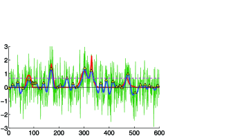
Figure 1: Simulated observed sequence $y(t)$ (green) and smoothed sequence $y_{\gamma}(t)$ (blue) over five underlying true peaks of different shapes comprising $\mu(t)$ (red). Out of 33 local maxima of $y_{\gamma}(t)$ (yellow), the BH detection threshold at FDR level 0.2 (dashed magenta) selects five, one of which is a false positive. At this noise level, four out of five true peaks are detected. Note that this bandwidth is able to distinguish the overlapping peaks.

We study the theoretical properties of the above algorithm under a specific signal-plus-noise model and then relax these assumptions in the simulations. For Type I errors to be well defined, the signal is modeled as if composed of unimodal peak regions, each considered detected if a significant local maximum occurs inside its finite support. For simplicity, we concentrate on positive signals and one-sided tests, but this is not crucial. For tractability, the theory assumes that the observation noise follows a smooth stationary ergodic Gaussian process. This assumption permits an explicit formula for computing the $p$-values corresponding to local maxima of the observed process. The distribution of the height of a local maximum of a Gaussian process is not Gaussian but has a heavier tail, and its computation requires careful conditioning based on the calculus of Palm probabilities [Adler, Taylor and Worsley (2010), Cramér and Leadbetter (1967)].

An interesting and challenging aspect of inference for local maxima is the fact that the number of tests, equal to the number of observed local maxima, is random. The multiple testing literature usually assumes the number of tests to be fixed. We overcome this difficulty with an asymptotic argument for large search space, so that by ergodicity, the error behaves approximately as it would if the number of tests were equal to its expected value.

In order to achieve strong control of FWER and FDR, the asymptotics for large search space are combined with asymptotics for strong signal. The strong signal assumption asymptotically eliminates the false positives caused by the smoothed signal spreading into the null regions, by assuring that each signal peak region is represented by only one observed local maximum within the true domain with probability tending to one. The strong signal assumption is not restrictive in the sense that the search space may grow exponentially faster. Simulations show that error levels are maintained at finite search spaces and moderate signal strength.

Defining detection power as the expected fraction of true peaks detected, we prove that the algorithm is consistent in the sense that its power tends to one under the above asymptotic conditions. We find that the optimal smoothing kernel is approximately that which is closest in shape and bandwidth to the signal peaks to be detected, akin to the so-called matched filter theorem in signal processing [Pratt (1991), Simon (1995)]. This optimal bandwidth is much larger than the usual optimal bandwidth for nonparametric regression.

In one dimension, the problem of identifying significant local maxima is similar to that of peak detection in signal processing [e.g., Arzeno, Deng and Poon (2008), Baccus and Meister (2002), Brutti et al. (2005), Harezlak et al. (2008), Morris et al. (2006), Yasui et al. (2003)]. In this literature, though large, the detection threshold is predominantly chosen heuristically and conservatively. Our multiple testing viewpoint provides a formal mechanism for choosing the detection threshold, allowing detection under higher noise conditions. This view also eliminates the need to estimate an unknown number of peak location parameters, encountered in the signal estimation approach [Li and Speed (2000, 2004), O’Brien, Sinclair and Kramer (1994), Tibshirani et al. (2005)].

We illustrate our procedure with a data set of neural electrical recordings, where the objective is to detect action potentials representing cell activity [Baccus and Meister (2002), Segev et al. (2004)]. The noise parameters and signal peak shape are estimated from a training set and then applied to a test set for peak detection.

The data analysis and all simulations were implemented in Matlab.

2 Theory

2.1 The model

Consider the signal-plus-noise model

$$y(t)=\mu(t)+z(t),\qquad t\in\mathbb{R},$$ (1)

where the signal $\mu(t)$ is a train of unimodal positive peaks of the form

$$\mu(t)=\sum_{j=-\infty}^{\infty}a_{j}h_{j}(t),\qquad a_{j}>0,$$ (2)

and the peak shape $h_{j}(t)\geq 0$ has compact connected support $S_{j}=\{t\dvtx h_{j}(t)>0\}$ and unit action $\int_{S_{j}}h_{j}(t)\,dt=1$ for each $j$. Let $w_{\gamma}(t)\geq 0$ with bandwidth parameter $\gamma>0$ be a unimodal kernel with compact connected support and unit action. Convolving the process (1) with the kernel $w_{\gamma}(t)$ results in the smoothed process

$$y_{\gamma}(t)=w_{\gamma}(t)*y(t)=\int_{-\infty}^{\infty}w_{\gamma}(t-s)y(s)\,ds=\mu_{\gamma}(t)+z_{\gamma}(t),$$ (3)

where the smoothed signal and smoothed noise are defined as

$$\mu_{\gamma}(t)=w_{\gamma}(t)*\mu(t)=\sum_{j=-\infty}^{\infty}a_{j}h_{j,\gamma}(t),\qquad z_{\gamma}(t)=w_{\gamma}(t)*z(t).$$ (4)

For each $j$, the smoothed peak shape $h_{j,\gamma}(t)=w_{\gamma}(t)*h_{j}(t)\geq 0$ is unimodal and has compact connected support $S_{j,\gamma}$ and unit action. For each $j$, we require that $h_{j,\gamma}(t)$ is twice differentiable in the interior of $S_{j,\gamma}$ and has no other critical points within its support. For simplicity, the theory requires that the supports $S_{j,\gamma}$ do not overlap (but this is not required in practice, as shown via simulations in Section 3). The smoothed noise $z_{\gamma}(t)$ defined by (3) and (4) is assumed to be a zero-mean thrice differentiable stationary ergodic Gaussian process.

2.2 The STEM algorithm

Suppose we observe $y(t)$ defined by (1) in the segment $[-L/2,L/2]$, which contains $J$ peaks. We call the following procedure STEM (Smoothing and TEsting of Maxima).

Algorithm 1 ((STEM algorithm)).

(1) Kernel smoothing: construct the process (3), ignoring the boundary effects at $\pm L/2$. [(2)]

Candidate peaks: find the set of local maxima of $y_{\gamma}(t)$ in $[-L/2,L/2]$

$$\tilde{T}=\biggl{\{}t\in\biggl{[}-\frac{L}{2},\frac{L}{2}\biggr{]}\dvtx\dot{y}_{\gamma}(t)=\frac{dy_{\gamma}(t)}{dt}=0,\ddot{y}_{\gamma}(t)=\frac{d^{2}y_{\gamma}(t)}{dt^{2}}<0\biggr{\}}.$$ (5)

$p$-values: for each $t\in\tilde{T}$ compute the $p$-value $p_{\gamma}(t)$ for testing the (conditional) hypothesis

$$\mathcal{H}_{0}(t)\dvtx\mu(t)=0\quad\mbox{vs.}\quad\mathcal{H}_{A}(t)\dvtx\mu(t)>0,\qquad t\in\tilde{T}.$$

Multiple testing: let $\tilde{m}$ be the number of tested hypotheses, equal to the number of local maxima in $\tilde{T}$. Apply a multiple testing procedure on the set of $\tilde{m}$ $p$-values $\{p_{\gamma}(t),t\in\tilde{T}\}$, and declare significant all peaks whose $p$-values are smaller than the significance threshold.

Steps (1) and (2) above are well defined under the model assumptions (for data on a grid, local maxima are defined as points higher than their neighbors). Step (3) is detailed in Section 2.3 below. For step (4), we use the Bonferroni procedure to control FWER and the BH procedure to control FDR. To apply Bonferroni at level $\alpha$, declare significant all peaks whose $p$-values are smaller than $\alpha/\tilde{m}$. To apply BH at level $\alpha$, find the largest index $k$ for which the $i$th smallest $p$-value is smaller than $i\alpha/\tilde{m}$, and declare as significant the $k$ peaks with smallest $p$-values. Notice that, in contrast to the usual application of the Bonferroni and BH procedures, the number of tests $\tilde{m}$ is random.

2.3 $p$-values

Given the observed heights $y_{\gamma}(t)$ at the local maxima $t\in\tilde{T}$, the $p$-values in step (3) of Algorithm 1 are computed as

$$p_{\gamma}(t)=F_{\gamma}[y_{\gamma}(t)],\qquad t\in\tilde{T},$$ (6)

where

$$F_{\gamma}(u)=\mathrm{P}\{z_{\gamma}(t)>u|t\in\tilde{T}\}$$ (7)

denotes the right cumulative distribution function (cdf) of $z_{\gamma}(t)$ at the local maxima $t\in\tilde{T}$, evaluated under the complete null hypothesis $\mu(t)=0,\forall t$.

The conditional distribution (7) is called a Palm distribution [Adler, Taylor and Worsley (2010), Chapter 6]. Unlike the marginal distribution of $z_{\gamma}(t)$, it is not Gaussian but stochastically greater. This is because the point of evaluation $t\in\tilde{T}$ is not a fixed point $t\in\mathbb{R}$, but the random location of a local maximum of $z_{\gamma}(t)$. Moreover, the conditioning event has probability zero. The Palm distribution (7) has a closed-form expression, originally obtained by Cramér and Leadbetter [(1967), Chapter 11] (equation 11.6.14), using the well-known Kac–Rice formula [Rice (1945), Adler and Taylor (2007), Chapter 11]. A direct application, borrowing notation from those sources, gives the following.

Proposition 2

Suppose the assumptions of Section 2.1 hold and that $\mu(t)=0,\forall t$. Define the moments

$$\sigma^{2}_{\gamma}=\operatorname{var}[z_{\gamma}(t)],\qquad\lambda_{2,\gamma}=\operatorname{var}[\dot{z}_{\gamma}(t)],\qquad\lambda_{4,\gamma}=\operatorname{var}[\ddot{z}_{\gamma}(t)].$$ (8)

Then the distribution (7) is given by

$$F_{\gamma}(u)=1-\Phi\Biggl{(}u\sqrt{\frac{\lambda_{4,\gamma}}{\Delta}}\Biggr{)}+\sqrt{\frac{2\pi\lambda^{2}_{2,\gamma}}{\lambda_{4,\gamma}\sigma^{2}_{\gamma}}}\phi\biggl{(}\frac{u}{\sigma_{\gamma}}\biggr{)}\Phi\Biggl{(}u\sqrt{\frac{\lambda^{2}_{2,\gamma}}{\Delta\sigma_{\gamma}^{2}}}\Biggr{)},$$ (9)

where $\Delta=\sigma^{2}_{\gamma}\lambda_{4,\gamma}-\lambda_{2,\gamma}^{2}$, and $\phi(x)$, $\Phi(x)$ are the standard normal density and cdf, respectively.

The quantities $\sigma^{2}_{\gamma}$, $\lambda_{2,\gamma}$ and $\lambda_{4,\gamma}$ in Proposition 2 depend on the kernel $w_{\gamma}(t)$ and the autocorrelation function of the original noise process $z(t)$. Explicit expressions may be obtained, for instance, for the following Gaussian autocorrelation model, which we use later in the simulations.

Example 3 ((Gaussian autocorrelation model)).

Let the noise $z(t)$ in (1) be constructed as

$$z(t)=\sigma\int_{-\infty}^{\infty}\frac{1}{\nu}\phi\biggl{(}\frac{t-s}{\nu}\biggr{)}\,dB(s),\qquad\sigma,\nu>0,$$

where $B(s)$ is standard Brownian motion and $\nu>0$. Convolving with a Gaussian kernel $w_{\gamma}(t)=(1/\gamma)\phi(t/\gamma)$ with $\gamma>0$ as in (4) produces a zero-mean infinitely differentiable stationary ergodic Gaussian process

$$z_{\gamma}(t)=w_{\gamma}(t)*z(t)=\sigma\int_{-\infty}^{\infty}\frac{1}{\xi}\phi\biggl{(}\frac{t-s}{\xi}\biggr{)}\,dB(s),\qquad\xi=\sqrt{\gamma^{2}+\nu^{2}},$$

with moments (8) given by $\sigma^{2}_{\gamma}=\sigma^{2}/(2\sqrt{\pi}\xi)$, $\lambda_{2,\gamma}=\sigma^{2}/(4\sqrt{\pi}\xi^{3})$, $\lambda_{4,\gamma}=3\sigma^{2}/(8\sqrt{\pi}\xi^{5})$. The above expressions may be used as approximations if the kernel, required to have finite support, is truncated at $t=\pm\gamma d$ for moderately large $d$, say $d=3$.

2.4 Error definitions

Because truly detected peaks may be shifted with respect to the true peaks as a result of noise, we define a significant local maximum to be a true positive if it falls anywhere inside the support of a true peak. Conversely, we define it to be a false positive if it falls outside the support of any true peak. Assuming the model of Section 2.1, define the signal region $\mathbb{S}_{1}$ and null region $\mathbb{S}_{0}$, respectively, by

$$\mathbb{S}_{1}=\bigcup_{j=1}^{J}S_{j}\quad\mbox{and}\quad\mathbb{S}_{0}=\biggl{[}-\frac{L}{2},\frac{L}{2}\biggr{]}\Bigm{\backslash}\Biggl{(}\bigcup_{j=1}^{J}S_{j}\Biggr{)}.$$ (10)

For a significance threshold $u$, the total number of detected peaks and the number of falsely detected peaks are

$$R(u)=\#\{t\in\tilde{T}\dvtx y_{\gamma}(t)>u\}\quad\mbox{and}\quad V(u)=\#\{t\in\tilde{T}\cap\mathbb{S}_{0}\dvtx y_{\gamma}(t)>u\},$$

respectively. Both are defined as zero if $\tilde{T}$ is empty. The FWER is defined as the probability of obtaining at least one falsely detected peak

$$\qquad\operatorname{FWER}(u)=\mathrm{P}\{V(u)\geq 1\}=\mathrm{P}\Bigl{\{}\tilde{T}\cap\mathbb{S}_{0}\neq\varnothing\mbox{ and }\max_{t\in\tilde{T}\cap\mathbb{S}_{0}}y_{\gamma}(t)>u\Bigr{\}}.$$ (11)

The FDR is defined as the expected proportion of falsely detected peaks

$$\operatorname{FDR}(u)=\mathrm{E}\biggl{\{}\frac{V(u)}{R(u)\vee 1}\biggr{\}}.$$ (12)

Figure 2: Schematic signal and null regions, before and after smoothing, in the vicinity of one signal peak.

Note that the above definitions are with respect to the original signal support $\mathbb{S}_{1}$, while the inference is carried out using the smoothed observed process $y_{\gamma}(t)$. Kernel smoothing enlarges the signal support and increases the probability of obtaining false positives in the null regions neighboring the signal [Perone Pacifico et al. (2007)]. In contrast to (10), the smoothed signal region $\mathbb{S}_{1,\gamma}\supset\mathbb{S}_{1}$ and smoothed null region $\mathbb{S}_{0,\gamma}\subset\mathbb{S}_{0}$ are

$$\mathbb{S}_{1,\gamma}=\bigcup_{j=1}^{J}S_{j,\gamma}\quad\mbox{and}\quad\mathbb{S}_{0,\gamma}=\biggl{[}-\frac{L}{2},\frac{L}{2}\biggr{]}\Bigm{\backslash}\Biggl{(}\bigcup_{j=1}^{J}S_{j,\gamma}\Biggr{)},$$ (13)

respectively (Figure 2). We call the difference between the expanded signal support and the true signal support the transition region

$$\mathbb{T}_{\gamma}=\mathbb{S}_{1,\gamma}\setminus\mathbb{S}_{1}=\mathbb{S}_{0}\setminus\mathbb{S}_{0,\gamma}=\bigcup_{j=1}^{J}T_{j,\gamma},$$ (14)

where $T_{j,\gamma}=S_{j,\gamma}\setminus S_{j}$ is the transition region corresponding to each peak $j$.

In general, a true peak may produce more than one significant local maximum, affecting the interpretation of definition (12) and the nonasymptotic validity of the FDR controlling procedure. However, as explained below, this multiplicity is unlikely to occur for strong signals, assuring validity at least asymptotically under that regime. The simulations of Section 3.1 show it not to be problematic in nonasymptotic situations for moderate signals and appropriate smoothing.

2.5 Strong control of FWER

In Algorithm 1, step (3) produces a list of $\tilde{m}$ $p$-values. If the Bonferroni correction is applied in step (4) with level $\alpha\in(0,1)$, then the null hypothesis $\mathcal{H}_{0}(t)$ at $t\in\tilde{T}$ is rejected if

$$p_{\gamma}(t)<\frac{\alpha}{\tilde{m}}\quad\iff\quad y_{\gamma}(t)>\tilde{u}_{\operatorname{Bon}}=F_{\gamma}^{-1}\biggl{(}\frac{\alpha}{\tilde{m}}\biggr{)},$$ (15)

where $\alpha/\tilde{m}$ is defined as 1 if $\tilde{m}=0$. Recall that, in contrast to the usual Bonferroni algorithm, the number of $p$-values $\tilde{m}$ is random.

Define the conditions: [(C2)]

The assumptions of Section 2.1 hold.

$L\to\infty$ and $a=\inf_{j}a_{j}\to\infty$, such that $(\log L)/a^{2}\to 0$ and $J/L\to A_{1}$ with $0<A_{1}<1$.

Theorem 4

Suppose that Algorithm 1 is applied with the Bonferroni threshold $\tilde{u}_{\operatorname{Bon}}$ (15). Then, under conditions (C1) and (C2),

$$\limsup\operatorname{FWER}(\tilde{u}_{\operatorname{Bon}})\leq\alpha.$$

The proof of Theorem 4 is given in Section 6.2. The large search space assumption in (C2) solves the problem of $\tilde{m}$ being random, implying that by the weak law of large numbers, the ratio $\tilde{m}/L$ is close to its expectation $\mathrm{E}[\tilde{m}/L]$ for large $L$. Thus the Bonferroni procedure with random threshold (15) has asymptotically the same error control properties as if the threshold were deterministic and equal to

$$u_{\operatorname{Bon}}^{*}=F_{\gamma}^{-1}\biggl{(}\frac{\alpha}{\mathrm{E}[\tilde{m}]}\biggr{)}\approx F_{\gamma}^{-1}\biggl{(}\frac{\alpha/L}{A_{1}+\mathrm{E}[\tilde{m}_{0,\gamma}(0,1)]}\biggr{)},$$ (16)

where

$$\mathrm{E}[\tilde{m}_{0,\gamma}(0,1)]=\frac{1}{2\pi}\sqrt{\frac{\lambda_{4,\gamma}}{\lambda_{2,\gamma}}}$$ (17)

is the expected number of local maxima of $z_{\gamma}(t)$ in the unit interval $(0,1)$ [Cramér and Leadbetter (1967), Chapter 10].

The strong signal assumption in (C2) implies (Lemma 10 in Section 6.1) that, with probability tending to 1, no local maxima are obtained in the transition region $\mathbb{T}_{\gamma}$ (14), and exactly one local maxima is obtained for each signal peak in $\mathbb{S}_{1}$. This avoids the error inflation due to smoothing and provides the approximation in (16). The proof of Lemma 10 shows that the asymptotic rates are exponential and controlled partially by the smallest absolute derivative of the smoothed peak shape in the transition region and the curvature of the smoothed peak shape at the mode.

2.6 Control of FDR

Suppose the BH procedure is applied in step (4) of Algorithm 1. For a fixed $\alpha\in(0,1)$, let $k$ be the largest index for which the $i$th smallest $p$-value is less than $i\alpha/\tilde{m}$. Then the null hypothesis $\mathcal{H}_{0}(t)$ at $t\in\tilde{T}$ is rejected if

$$p_{\gamma}(t)<\frac{k\alpha}{\tilde{m}}\quad\iff\quad y_{\gamma}(t)>\tilde{u}_{\operatorname{BH}}=F_{\gamma}^{-1}\biggl{(}\frac{k\alpha}{\tilde{m}}\biggr{)},$$ (18)

where $k\alpha/\tilde{m}$ is defined as 1 if $\tilde{m}=0$.

Theorem 5

Suppose that Algorithm 1 is applied with the BH threshold $\tilde{u}_{\operatorname{BH}}$ (18). Then, under conditions (C1) and (C2),

$$\limsup\operatorname{FDR}(\tilde{u}_{\operatorname{BH}})\leq\alpha.$$

The proof of Theorem 5 is given in Section 6.3. The asymptotic assumptions (C2), imply that the BH procedure with random threshold (18) has asymptotically the same error control properties as if the threshold were deterministic and equal to

$$u^{*}_{\operatorname{BH}}=F_{\gamma}^{-1}\biggl{(}\frac{\alpha A_{1}}{A_{1}+\mathrm{E}[\tilde{m}_{0,\gamma}(0,1)](1-\alpha)}\biggr{)},$$ (19)

where $\mathrm{E}[\tilde{m}_{0,\gamma}(0,1)]$ is given by (17). The threshold (18) can be viewed as the largest solution of the equation $\alpha G(u)=F_{\gamma}(u)$, where $G(u)$ is the empirical right cumulative distribution function of $y_{\gamma}(t),t\in\tilde{T}$ [Genovese, Lazar and Nichols (2002)]. Taking the limit of that equation as $L$ gets large yields the solution (19).

As before, the strong signal assumption in (C2) implies that there exists exactly one significant local maximum at each true peak with probability tending to 1 (Lemma 10 in Section 6.1), avoiding error inflation in the transition region and justifying the interpretation of definition (12) as the expected proportion of falsely discovered peaks. Again, the asymptotic rates are exponential and controlled partially by the smallest absolute derivative of the smoothed peak shape in the transition region and the curvature of the smoothed peak shape at the mode.

Notice that, in contrast to the asymptotic Bonferroni threshold $u^{*}_{\operatorname{Bon}}$ (16) which grows unbounded with increasing $L$, the asymptotic BH thresh-old $u^{*}_{\operatorname{BH}}$ (19) is finite.

2.7 Power

Recall from Section 2.4 that a significant local maximum is considered a true positive if it falls in the true signal region $\mathbb{S}_{1}$. We define the power of Algorithm 1 as the expected fraction of true discovered peaks

$$\operatorname{Power}(u) = \mathrm{E}\Biggl{[}\frac{1}{J}\sum_{j=1}^{J}1\Bigl{(}\tilde{T}\cap S_{j}\neq\varnothing\mbox{ and }\max_{\tilde{t}\in\tilde{T}\cap S_{j}}y_{\gamma}(\tilde{t})>u\Bigr{)}\Biggr{]}$$

$$= \frac{1}{J}\sum_{j=1}^{J}\operatorname{Power}_{j}(u),$$

where $\operatorname{Power}_{j}(u)$ is the probability of detecting peak $j$

$$\operatorname{Power}_{j}(u)=\mathrm{P}\Bigl{\{}\tilde{T}\cap S_{j}\neq\varnothing\mbox{ and }\max_{t\in\tilde{T}\cap S_{j}}y_{\gamma}(t)>u\Bigr{\}}.$$ (21)

The maximum operator above indicates that if more than one significant local maximum fall within the same peak support, only one is counted, so power is not inflated. However, this has no effect asymptotically because each true peak is represented by exactly one local maximum of the smoothed observed process with probability tending to 1 (Lemma 10 in Section 6.1). The next result indicates that both the Bonferroni and BH procedures are asymptotically consistent. The proof is given in Section 6.4.

Theorem 6

Let the power be defined by (2.7), and let $\tilde{u}_{\operatorname{Bon}}$ and $\tilde{u}_{\operatorname{BH}}$ be the Bonferroni and BH thresholds (15) and (18), respectively. Under conditions (C1) and (C2),

$$\operatorname{Power}(\tilde{u}_{\operatorname{Bon}})\to 1,\qquad\operatorname{Power}(\tilde{u}_{\operatorname{BH}})\to 1.$$

For pointwise tests, if there exists a signal anywhere, the BH procedure is more powerful than the Bonferroni procedure [Benjamini and Hochberg (1995)]. This is also true in our case. Comparing (16) and (19), if $J\geq 1$, the threshold $u^{*}_{\operatorname{Bon}}$ is higher than the threshold $u^{*}_{\operatorname{BH}}$, promising a larger power for the BH procedure.

2.8 Optimal smoothing kernel

The best smoothing kernel $w_{\gamma}(t)$ is that which maximizes the power (2.7) under the true model. Because this maximization is analytically difficult, we resort to a less formal argument here. Lemma 10 in Section 6.1 shows that, under conditions (C1) and (C2), every true peak $j$ is represented by exactly one significant local maximum located in a small neighborhood containing the true peak mode $\tau_{j}$ with probability tending to 1. Thus the power for peak $j$ (21) may be approximated as

$$\operatorname{Power}_{j}(u)\approx\mathrm{P}\{y_{\gamma}(\tau_{j})>u\}=\Phi\biggl{[}\frac{a_{j}h_{j,\gamma}(\tau_{j})-u}{\sigma_{\gamma}}\biggr{]},$$ (22)

because $y_{\gamma}(\tau_{j})\sim N(a_{j}h_{j,\gamma}(\tau_{j}),\sigma_{\gamma}^{2})$. By Lemma 13 in Section 6.4, the asymptotically equivalent thresholds (16) and (19) for the Bonferroni and BH procedures satisfy $u^{*}_{\operatorname{Bon}}/a_{j}\to 0$ and $u^{*}_{\operatorname{BH}}/a_{j}\to 0$ for any $j$. Thus, for large $a_{j}$, the power (22) is maximized approximately by maximizing the SNR

$$\operatorname{SNR}_{\gamma}=\frac{a_{j}h_{j,\gamma}(\tau_{j})}{\sigma_{\gamma}}=\frac{a_{j}\int_{-\infty}^{\infty}w_{\gamma}(s)h_{j}(s)\,ds}{\sigma\sqrt{\int_{-\infty}^{\infty}w^{2}_{\gamma}(s)\,ds}},$$ (23)

where $\sigma$ is the standard deviation of the observed process $y(t)$. The optimal smoothing kernel $w_{\gamma}(t)$ is that which is closest to $h_{j}(t)$ in an $L_{2}$ sense. This result is similar to the matched filter theorem for detecting a single signal peak of known shape at a fixed time location $t$ [Pratt (1991), Simon (1995)]. The result only holds approximately in our case because the peak locations are unknown.

Example 7 ((Gaussian autocorrelation model)).

Suppose the signal peak $j$ is a truncated Gaussian density $h_{j}(t)=(1/b_{j})\phi[(t-\tau_{j})/b_{j}]\mathbf{1}[-c_{j},c_{j}]$, $b_{j},\break c_{j}>0$, and let the noise be generated as in Example 3. Ignoring the truncation, $h_{j,\gamma}(t)=w_{\gamma}(t)*h_{j}(t)$ in (23) is the convolution of two Gaussian densities with variances $\gamma^{2}$ and $b_{j}^{2}$, which is another Gaussian density with variance $\gamma^{2}+b_{j}^{2}$. Using the moments from Example 3, we have that

$$\operatorname{SNR}_{\gamma}=\frac{a_{j}h_{j,\gamma}(\tau_{j})}{\sigma_{\gamma}}=\frac{a_{j}}{\sigma\pi^{1/4}}\biggl{[}\frac{\gamma^{2}+\nu^{2}}{(\gamma^{2}+b_{j}^{2})^{2}}\biggr{]}^{1/4}.$$ (24)

As a function of $\gamma$, the SNR is maximized at

$$\mathop{\arg\max}_{\gamma}\operatorname{SNR}_{\gamma}=\cases{\sqrt{b_{j}^{2}-2\nu^{2}},&\quad$\nu<b_{j}/\sqrt{2}$,\cr 0,&\quad$\nu>b_{j}/\sqrt{2}$.}$$ (25)

In particular, when $\nu=0$, we have that the optimal bandwidth for peak $j$ is $\gamma=b_{j}$, the same as the signal bandwidth. We show in the simulations below that the optimal $\gamma$ is indeed close to (25).

3 Simulation studies

3.1 Nonasymptotic performance

Simulations were used to evaluate the performance and limitations of the STEM algorithm for finite range $L$ and moderate signal strength $a$. In a segment of length $L=1000$, $J=10$ equal truncated Gaussian peaks $a_{j}h_{j}(t)=a/b\phi[(t-\tau_{j})/b]\mathbf{1}[-cb,cb]$, $j=1,\ldots,J$, as in Example 7 with $b=3$, $c=3$ and varying $a$, were placed at uniformly spaced locations $\tau_{j}=(j-1/2)L/J$, $j=1,\ldots,J$, and sampled at integer values of $t$. The noise $z(t)$ was constructed as in Example 3 with $\sigma=1$ and varying $\nu$. Algorithm 1 was carried out using as smoothing kernel a truncated Gaussian density $w_{\gamma}(t)=(1/\gamma)\phi(t/\gamma)\mathbf{1}[-c\gamma,c\gamma]$ as in Example 3 with $c=3$ and varying $\gamma$. The noise parameters (8) were estimated independently as the empirical moments of smoothed sequences i.i.d. Gaussian noise of length 1000 and their first and second-order differences, using the same smoothing kernel. The Bonferroni and BH procedures were applied at level $\alpha=0.05$.

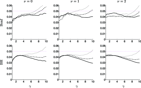
Figure 3: FWER of the Bonferroni procedure (top row) and FDR of the BH procedure (bottom row) for $a=15$ (solid), $a=12$ (dashed) and $a=9$ (dotted). Nominal error level is 0.05.

Figure 3 shows the realized FWER and FDR levels of the Bonferroni and BH procedures, evaluated according to (11) and (12) with the expectations replaced by ensemble averages over 10,000 replications. Error rates are maintained below the nominal level $\alpha=0.05$ for all bandwidths and large enough signal strength $a$. The convergence is slower, however, when the bandwidth $\gamma$ is much larger than the signal peak bandwidth $b=3$. The increased error rates are the result of true peak maxima being shifted from the original signal region $\mathbb{S}_{1}$ into the transition region $\mathbb{T}_{\gamma}$, where they are counted as false positives. This phenomenon disappears with increasing signal strength $a$ because the probability of obtaining any local maxima in the transition region goes to zero asymptotically (Lemma 10 in Section 6.1).

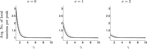
Figure 4: Average number of local maxima for each true peak for $a=15$ (solid), $a=12$ (dashed) and $a=9$ (dotted).

As noted in Section 2.4, each true peak may contain more than one local maximum of the smoothed data $y_{\gamma}(t)$. Figure 4 shows that the expected number of local maxima per true peak decreases with increasing bandwidth, and is essentially equal to 1 for bandwidths equal to or greater than the optimal bandwidth. It also gets closer to 1 with increasing signal strength, consistent with the result of Lemma 10.

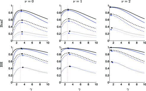
Figure 5: Realized (black) and “theoretical” (blue) power of the Bonferroni (top row) and BH (bottom row) procedures for $a=15$ (solid), $a=12$ (dashed) and $a=9$ (dotted). The maxima of the curves (solid circles) approach the asymptotic optimal bandwidth (vertical dashed).

Figure 5 shows the realized power of the Bonferroni and BH procedures, evaluated according to (2.7) with the expectations replaced by ensemble averages over the same 10,000 replications. In all cases, the power increases asymptotically to 1 with the signal strength for every fixed bandwidth, and is always larger for BH than it is for Bonferroni. The convergence is slower, however, when the bandwidth $\gamma$ is far from the optimal value. To understand the dependence on bandwidth, superimposed is the theoretical approximate power (22) evaluated at the asymptotic thresholds $u^{*}_{\operatorname{Bon}}$ (16) and $u^{*}_{\operatorname{BH}}$ (19) and plugging in the SNR (24). The “theoretical” power curves largely capture the shape of the realized ones, but are lower because the asymptotic thresholds are more conservative. The curve shape is mostly determined by the SNR (24) as a function of $\gamma$. The bandwidth $\gamma$ producing the largest power is always larger than the theoretical optimal bandwidth (25), but it approaches it from the right as $a$ increases.

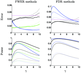
Figure 6: Left panels: FWER and power of three FWER methods: STEM with Bonferroni (black), Bonferroni on all $L$ locations (blue) and Supremum (green). Right panels: FDR and power of three FDR methods: STEM with BH (black), BH on all $L$ locations (blue). Results in all panels are for $a=15$ (solid), $a=12$ (dashed) and $a=9$ (dotted). Nominal error level is 0.05.

3.2 Unequal peaks

By assumption (Section 2.1), the signal peaks need not be equal. As in Figure 1, $J=5$ unequal peaks (Epanechnikov, triangular and truncated Gaussian, Laplace and Cauchy, with average half-support 24) were corrupted with white standard normal noise. Algorithm 1 was applied using a quartic smoothing kernel $w_{\gamma}(t)=15/(16\gamma)[1-(t/\gamma)^{2}]^{2}\mathbf{1}[-\gamma,\gamma]$ with varying $\gamma$, the noise parameters estimated independently as in Section 3.1. For this configuration and 10,000 repetitions, the error was controlled below the nominal level 0.05 for values of $\gamma$ up to 40, obtaining a maximum power of 0.81 and 0.88 for the Bonferroni and BH procedures at $\gamma=18$. The maximizing bandwidth represents the average best match between the quartic smoothing kernel and the peaks present in the data.

3.3 Overlapping peaks

The theory of Section 2 assumed that the signal peaks had nonoverlapping supports. Simulations similar to those of Section 3.1 with $J=10$ partially overlapping peaks showed that the error rates were below the nominal level regardless of the amount of overlap between peaks. The detection power, however, deceptively increased with increasing overlap. This is because definition (2.7) counts two overlapping peaks as detected even if only one significant local maximum is found in the overlapping region between them, as it belongs to both. Definition (2.7) does not measure the ability to distinguish between overlapping peaks.

3.4 Comparison with pointwise testing

To see the benefits of testing local maxima, Figure 6 compares the performance of the STEM algorithm (with Bonferroni and BH corrections) to three other methods that test at every single location. Simulated data sets as in Section 3.1 with $b=3$ and $\nu=0$ were smoothed with varying $\gamma$. For the pointwise Bonferroni and BH methods, $p$-values for testing $H_{0}\dvtx\mu(t)=0$ at each $t=1,\ldots,L=1000$ were computed as $p(t)=1-\Phi[y_{\gamma}(t)/\sigma_{\gamma}]$ and then corrected using Bonferroni and BH, respectively. The method “Supremum” was adapted from Worsley et al. (1996a) as follows. The probability that the supremum of any differentiable random process $f(t)$ in the interval $[0,T]$ exceeds $u$ is bounded by [Adler and Taylor (2007)]

$$\mathrm{P}\Bigl{(}\sup_{t\in[0,T]}f(t)\geq u\Bigr{)}\leq\mathrm{P}[f(0)\geq u]+\mathrm{E}[N_{u}],$$ (26)

where $N_{u}$ is the number of up-crossings by $f(t)$ of the level $u$ in $[0,T]$. For the stationary Gaussian process $z_{\gamma}(t)$, application of the Kac–Rice formula [Cramér and Leadbetter (1967), page 194] gives that $\mathrm{E}[N_{u}]=L(\sqrt{\lambda_{2,\gamma}}/\allowbreak\sigma_{\gamma})\phi(u/\sigma_{\gamma})$. The significance threshold is found as the largest $u$ such that

$$\mathrm{P}\Bigl{(}\sup_{t\in[-L/2,L/2]}z_{\gamma}(t)\geq u\Bigr{)}\leq 1-\Phi\biggl{(}\frac{u}{\sigma_{\gamma}}\biggr{)}+L\frac{\sqrt{\lambda_{2,\gamma}}}{\sigma_{\gamma}}\phi\biggl{(}\frac{u}{\sigma_{\gamma}}\biggr{)}\leq\alpha.$$ (27)

Figure 6 indicates that the pointwise Bonferroni correction is too conservative. The Supremum method, despite accounting explicitly for the noise autocorrelation, performs only slightly better than pointwise Bonferroni, and not as well as Bonferroni performed on local maxima. The pointwise BH correction is designed to control FDR at the level of individual locations, and thus produces too many false positives when the FDR is measured in terms of detected peaks using (12). Further simulations with $\nu=1$ and $\nu=2$ yielded similar results (not shown).

3.5 Automatic bandwidth selection

Rather than using a fixed smoothing bandwidth $\gamma$, the bandwidth may be chosen automatically from the data as the one that yields the largest number of discoveries for a fixed error level. For simulated data sets as in Section 3.1 with $b=3$ and $\nu=0$, the STEM algorithm was applied with $\gamma$ ranging from $\gamma=b/2=1.5$ to $\gamma=2b=6$, and results were retained for the bandwidth $\hat{\gamma}$ that yielded the largest number of discoveries in each run. Figure 7(a) shows that this automatic criterion biases the results toward more detected peaks and therefore results in higher

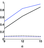
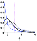
(a)	(b)

Figure 7: (a) Power (solid) and realized error rate (dashed) for Bonferroni (black) and BH (blue) with automatic bandwidth selection as a function of signal strength $a$. Nominal error level is 0.05. (b) Proportion of automatically chosen smoothing bandwidth $\hat{\gamma}$ over 1000 simulations for Bonferroni (black) and BH (blue); results are for $a=15$ (solid), $a=12$ (dashed) and $a=9$ (dotted). Nominal optimal bandwidth is $\gamma=3$.

error rates (and power) than those obtained when $\gamma$ is fixed (Figure 5). It also tends to select bandwidths that are smaller than the nominal optimal value $\gamma=b$ [Figure 7(b)], with averages ranging between about 2.1 and 2.9.

4 Data example

The data consists of recordings from a single electrode inserted in a salamander’s retina, digitized at a sampling frequency of 10 kHz. Data of these kind are routinely collected in large amounts in neuroscience experiments [Baccus and Meister (2002), Segev et al. (2004)]. For the purposes of this paper, three data sets were used: [(3)]

Test set: 60 seconds of recordings of live cells in the dark.

Training set 1: 60 seconds of recordings of live cells in the dark.

Training set 2: 60 seconds of recordings after the retina was allowed to die. Each period of 60 seconds corresponds to $L=6\times 10^{5}$ samples. The goal of the analysis was to detect neuronal spikes in the test set (Figure 8, top left).

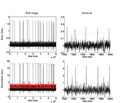
Figure 8: Top row: the neural spike data (test set); the stars in the right panel indicate peaks that are higher than 4 standard deviations of the raw data (dashed line), as suggested by Segev et al. (2004). Bottom row: the data smoothed using the estimated peak shape as kernel; the stars indicate significant local maxima higher than the BH threshold (magenta dashed line) at level 0.01. The Bonferroni threshold is indicated by the cyan dashed line.

Assuming that neuronal action potentials have similar shapes, to maximize the SNR (23), the smoothing filter should be close in shape and bandwidth to that of the peaks to be detected. Training set 1 was used to estimate the peak shape. In training set 1, spikes with raw maximum exceeding 1 were selected and aligned by their maxima [Figure 9(a)]. The peak shape template was obtained as the average of the 23 selected major spikes and truncated to a length of 100 samples.

Training set 2, recorded under pure noise conditions, was used to estimate the noise parameters. The noise in training set 2 can be well modeled by an AR(3) process with autoregressive coefficients $-$1.13, 0.42 and $-$0.13, estimated by the Yule–Walker algorithm, so that whitening with these coefficients produces a process whose autocovariance function cannot be distinguished from that of white noise using a Bartlett’s test. A similar analysis in segments of length $L/10$ showed that the estimated AR coefficients have a coefficient of variation of no more than 1% over the 10 segments, supporting the stationarity assumption. A Jarque–Bera test of normality for the entire sequence returned a $p$-value of 0.224, supporting the Gaussianity assumption.

Convolving training set 2 with the template of Figure 9(a) produced smoothed noise with spectral moments $\hat{\sigma}_{\gamma}^{2}=4.22\times 10^{-4}$, $\hat{\lambda}_{2,\gamma}^{2}=1.20\times 10^{-4}$ and $\hat{\lambda}_{4,\gamma}^{2}=1.96\times 10^{-4}$, estimated respectively by the empirical variances of the observed process, its first-order difference and its second-order difference. Given the length of the process, the standard error of these estimates is negligible.

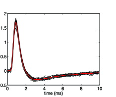
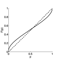
(a)	(b)

Figure 9: (a) 23 strongest spikes aligned by their maximum (black); their average (red) is the estimated template. (b) Empirical cdf of $p$-values for the test set (solid) and training set 2 (dashed).

Algorithm 1 was applied to the test set (Figure 8, top left) by convolving it with the template of Figure 9(a), producing the smoothed process in Figure 8 (bottom left). In $L=6\times 10^{5}$ samples, $\tilde{m}=30\mbox{,}426$ local maxima were found and their $p$-values were computed according to (6) and (9), plugging in the estimates $\hat{\sigma}_{\gamma}^{2}$, $\hat{\lambda}_{2,\gamma}^{2}$ and $\hat{\lambda}_{4,\gamma}$ found above. The empirical cdf of the $p$-values [Figure 9(b)] shows a large fraction of nonnull $p$-values near 0. For comparison, the same procedure of smoothing, finding local maxima and computing their $p$-values was applied to training set 2. The empirical cdf of those $p$-values is virtually uniform, emphasizing that formula (9) for Gaussian noise is appropriate. Also in Figure 9(b), the excess of large $p$-values from the test set is due to the negative portions of the smoothing function [Figure 9(a)]. These produce small negative anti-spikes whose $p$-values are large when tested for positiveness.

Applying the BH procedure to the $\tilde{m}=30\mbox{,}426$ $p$-values obtained from the test set at FDR level 0.01 resulted in a $p$-value threshold of $2.76\times 10^{-4}$ and $R=843$ significant local maxima. These are indicated in Figure 8 (bottom left), showing three levels of spike strengths. Figure 8 (bottom right) zooms in to show a few of the weaker spikes. Applying the Bonferroni procedure instead in Algorithm 1 resulted in a $p$-value threshold of $3.29\times 10^{-7}$ and only 411 detected spikes.

For comparison, Figure 8 (top right) shows the same segment of the raw data and the spikes selected using one of the recommended methods in the neuroscience literature, which is to threshold at 4 standard deviations of the raw data [Segev et al. (2004)]. Our method is able to identify more spikes at a low FDR level of 0.01, but more importantly, it attaches to the findings a significance level, expecting about 1% of the detected spikes to be false. The conventional method does not offer this useful statistical interpretation.

As in Section 3.4, computing $p$-values at each location as $p(t)=1-\Phi(y_{\gamma}(t)/\hat{\sigma}_{\gamma})$, $t=1,\ldots,L$, and applying a global Bonferroni at level 0.01 was more conservative, resulting in a height threshold of 1.235 (comparable to Figure 8 bottom right) and detecting only 393 spikes. Similarly, the “Supremum” method, applied by replacing $\hat{\sigma}_{\gamma}$ and $\hat{\lambda}_{\gamma}$ in (27) at level 0.01, yielded a height threshold 1.229 and 394 detected spikes. Finally, applying the global BH procedure at level 0.01 with $L$ $p$-values gave a height threshold of 0.780 detecting 1149 spikes, but as shown in Section 3.4, this result is too optimistic because the actual error rate for peaks is higher than 0.01.

5 Discussion

For the theoretical results, the most critical assumptions were that the noise process is stationary ergodic Gaussian and that the signal peaks are unimodal with compact support. The Gaussianity assumption was chosen because it enabled a closed formula for computing the $p$-values associated with the heights of local maxima. For non-Gaussian noise, $p$-values could be computed via Monte Carlo simulation.

The assumption of compact support for the signal peaks was necessary for true and false positives to be well defined. Chumbley et al. (2010) argued for testing local maxima when the signal spreads over the entire domain, but in that case every positive is a true positive, making the inference unclear. On the other hand, agreeing with Chumbley and Friston (2009), applying BH globally resulted in inflated error rates for peaks, while applying Bonferroni or the Supremum method globally was too conservative. The unimodality assumption made local maxima good representatives of true peaks, being unique for medium to large bandwidths and asymptotically for increasing signal strength.

The strong signal assumption in condition (C2) was introduced to remove the excess error produced by the smoothed signal spreading into the neighboring null regions, thereby enabling asymptotic error control. The assumption is not restrictive in the sense that the search space may grow exponentially faster. Similar conditions are common for high-dimensional data. If the data are pointwise test statistics based on a sample of size $n$, with SNR increasing as $a=\sqrt{n}\to\infty$, then the condition $(\log L)/a^{2}\to 0$ becomes $(\log L)/n\to 0$. This is similar to the condition $(\log p)/n\to 0$ required for consistent model selection in high-dimensional regression under sparsity where $p$ is the number of features [Candes and Tao (2007), Zhang (2010)]. Our results, however, do not require sparsity. Condition (C2) is easy to state but stronger than needed; upon close inspection of the proof of Lemma 10 in Section 6.1, the limit of $(\log L)/a^{2}$ need not be zero but need only be bounded by a constant that depends on the signal and noise first and second derivatives.

While the theory was developed for continuous processes, in practice the observations are given in a discrete grid. In our simulations we found that the results were not reliable when the smoothing bandwidth was smaller than the grid spacing, as the theory for continuous random processes is no longer a good approximation in that case.

The asymptotic error control and power consistency did not require the peaks to have the same shape or width. The asymptotic results were found to hold in practice for a wide range of bandwithds and strong enough signal. However, the convergence rate was slower for bandwidths less than half or more than double the optimal value. The matched filter principle suggests that the smoothing kernel should be chosen to be as close as possible in an $L^{2}$ sense to the peaks to be detected. In the neuronal data analyzed, the peak shape and width were estimated from the data, dictating the best smoothing kernel. If the peaks to be detected have different widths, then the bandwidth may be adapted to the width of each peak. We leave this possibility for future work, as well as the obliged extension of the proposed methods to two- and three-dimensional domains.

6 Technical details

6.1 Supporting results

Lemma 8

Let $\tilde{m}_{0,\gamma}=\#\{t\in\tilde{T}\cap\mathbb{S}_{0,\gamma}\}$ be be the number of local maxima of $y_{\gamma}(t)$ [or $z_{\gamma}(t)$] in $\mathbb{S}_{0,\gamma}$. Let $V_{\gamma}(u)=\#\{t\in\tilde{T}\cap\mathbb{S}_{0,\gamma}\dvtx y_{\gamma}(t)>u\}$ be the number of local maxima of $y_{\gamma}(t)$ [or $z_{\gamma}(t)$] in $\mathbb{S}_{0,\gamma}$ whose heights are above the level $u$. Then

$$\frac{V_{\gamma}(u)}{\tilde{m}_{0,\gamma}}\to\frac{\mathrm{E}[V_{\gamma}(u)]}{\mathrm{E}[\tilde{m}_{0,\gamma}]}=F_{\gamma}(u)$$

in probability as $L\to\infty$, where $F_{\gamma}(u)$ is the Palm distribution (7).

Notice that $y_{\gamma}(t)=z_{\gamma}(t)$ for all $t\in\mathbb{S}_{0,\gamma}$, so the process $y_{\gamma}(t)$ has the same properties as the stationary process $z_{\gamma}(t)$ on the set $\mathbb{S}_{0,\gamma}$. By ergodicity, the weak law of large numbers applied to the numerator and denominator gives that

$$\frac{V_{\gamma}(u)}{\tilde{m}_{0,\gamma}}=\frac{\#\{t\in\tilde{T}\cap\mathbb{S}_{0,\gamma}\dvtx z_{\gamma}(t)>u\}/L}{\#\{t\in\tilde{T}\cap\mathbb{S}_{0,\gamma}\}/L}$$ (28)

converges to [Cramér and Leadbetter (1967)]

$$\frac{\mathrm{E}[\#\{t\in\tilde{T}\cap\mathbb{S}_{0,\gamma}\dvtx z_{\gamma}(t)>u\}]}{\mathrm{E}[\#\{t\in\tilde{T}\cap\mathbb{S}_{0,\gamma}\}]}=\frac{\mathrm{E}[V_{\gamma}(u)]}{\mathrm{E}[\tilde{m}_{0,\gamma}]}.$$

But also by ergodicity, ratio (28) converges to the conditional probability $\mathrm{P}[z_{\gamma}(t)>u|t\in\tilde{T}\cap\mathbb{S}_{0,\gamma}]=F_{\gamma}(u)$ by Definition (7). The two limits must be equal.

Lemma 9

Assume the model of Section 2.1. Let $S_{j,\gamma}=I_{j}^{\mathrm{left}}\cup I_{j}^{\mathrm{mode}}\cup I_{j}^{\mathrm{right}}$ be a partition, where $I_{j}^{\mathrm{mode}}=[c_{j},d_{j}]\subset S_{j}$ is a fixed interval containing the mode of $\mu_{\gamma}(t)=a_{j}h_{j,\gamma}(t)$ in $S_{j}$ as an interior point, such that $\ddot{h}_{j,\gamma}(t)<0$ for $t\in I_{j}^{\mathrm{mode}}$, $\dot{h}_{j,\gamma}(t)>0$ for $t\in I_{j}^{\mathrm{left}}$ and $\dot{h}_{j,\gamma}(t)<0$ for $t\in I_{j}^{\mathrm{right}}$. Let:

• $M_{j}$ be the largest value of $|h_{j,\gamma}(t)|$ in $S_{j,\gamma}$;

• $C_{j}$ be the smallest value of $|\dot{h}_{j,\gamma}(t)|$ in $I_{j}^{\mathrm{side}}=I_{j}^{\mathrm{left}}\cup I_{j}^{\mathrm{right}}$;

• $D_{j}$ be the smallest value of $|\ddot{h}_{j,\gamma}(t)|$ in $I_{j}^{\mathrm{mode}}$.

For $\tilde{T}$ given by (5) and any threshold $u$,

$$\mathrm{P}(\#\{t\in\tilde{T}\cap I_{j}^{\mathrm{side}}\}=0)$$

$$\qquad\geq 2\Phi\biggl{(}\frac{a_{j}C_{j}}{\sqrt{\lambda_{2,\gamma}}}\biggr{)}-1-|I_{j}^{\mathrm{side}}|\sqrt{\frac{\lambda_{4,\gamma}}{\lambda_{2,\gamma}}}\phi\biggl{(}\frac{a_{j}C_{j}}{\sqrt{\lambda_{2,\gamma}}}\biggr{)},$$

$$\mathrm{P}(\#\{t\in\tilde{T}\cap I_{j}^{\mathrm{mode}}\}=1)$$

$$\qquad\geq\Phi\biggl{(}\frac{a_{j}D_{j}}{\sqrt{\lambda_{4,\gamma}}}\biggr{)}-|I_{j}^{\mathrm{mode}}|\sqrt{\frac{\lambda_{6,\gamma}}{\lambda_{4,\gamma}}}\phi\biggl{(}\frac{a_{j}D_{j}}{\sqrt{\lambda_{4,\gamma}}}\biggr{)}-2\Phi\biggl{(}\frac{-a_{j}C_{j}}{\sqrt{\lambda_{2,\gamma}}}\biggr{)},$$

$$\mathrm{P}\bigl{(}\#\{t\in\tilde{T}\cap I_{j}^{\mathrm{mode}}\dvtx y_{\gamma}(t)>u\}=1\bigr{)}$$

$$\qquad\geq\Phi\biggl{(}\frac{a_{j}D_{j}}{\sqrt{\lambda_{4,\gamma}}}\biggr{)}-|I_{j}^{\mathrm{mode}}|\sqrt{\frac{\lambda_{6,\gamma}}{\lambda_{4,\gamma}}}\phi\biggl{(}\frac{a_{j}D_{j}}{\sqrt{\lambda_{4,\gamma}}}\biggr{)}-\Phi\biggl{(}\frac{u-a_{j}M_{j}}{\sigma_{\gamma}}\biggr{)},$$

where $\sigma_{\gamma}$, $\lambda_{2,\gamma}$ and $\lambda_{4,\gamma}$ are given by (8) and $\lambda_{6,\gamma}=\mathrm{E}[\dot{\hphantom{z}}\ddot{\hphantom{0}}z_{\gamma}(t)]$.

(1) Consider first the compact interval $I_{j}^{\mathrm{left}}$. The probability that there are no local maxima of $y_{\gamma}(t)$ in $I_{j}^{\mathrm{left}}$ is greater than the probability that $\dot{y}_{\gamma}(t)>0$ for all $t$ in the interval. This probability is equal to

$$\mathrm{P}\Bigl{(}\inf_{I_{j}^{\mathrm{left}}}\dot{y}_{\gamma}(t)>0\Bigr{)} \geq \mathrm{P}\Bigl{(}\inf_{I_{j}^{\mathrm{left}}}\dot{z}_{\gamma}(t)>-\inf_{I_{j}^{\mathrm{left}}}\dot{\mu}_{\gamma}(t)\Bigr{)}$$

$$= 1-\mathrm{P}\Bigl{(}\sup_{I_{j}^{\mathrm{left}}}[-\dot{z}_{\gamma}(t)]>a_{j}C_{j}^{\mathrm{left}}\Bigr{)},$$

where $C_{j}^{\mathrm{left}}>0$ is the smallest value of $\dot{h}_{j,\gamma}(t)$ in $I_{j}^{\mathrm{left}}$. Inequality (26) applies above to the stationary Gaussian process $-\dot{z}_{\gamma}(t)$. The Kac–Rice formula [Cramér and Leadbetter (1967), page 194] gives in this case that $\mathrm{E}[N_{u}]=|I_{j}^{\mathrm{left}}|\sqrt{\lambda_{4,\gamma}}/\sqrt{\lambda_{2,\gamma}}\phi(u/\sqrt{\lambda_{2,\gamma}})$. Thus (6.1) has the lower bound

$$\mathrm{P}(\#\{t\in\tilde{T}\cap I_{j}^{\mathrm{left}}\}=0)\geq\Phi\biggl{(}\frac{a_{j}C_{j}^{\mathrm{left}}}{\sqrt{\lambda_{2,\gamma}}}\biggr{)}-|I_{j}^{\mathrm{left}}|\sqrt{\frac{\lambda_{4,\gamma}}{\lambda_{2,\gamma}}}\phi\biggl{(}\frac{a_{j}C_{j}^{\mathrm{left}}}{\sqrt{\lambda_{2,\gamma}}}\biggr{)}.$$

A similar calculation for $I_{j}^{\mathrm{right}}$ gives a similar bound with the superscript “left” replaced by “right” and $C_{j}^{\mathrm{right}}>0$ being the smallest value of $|\dot{h}_{j,\gamma}(t)|$ in $I_{j}^{\mathrm{right}}$. Putting the two together, the required probability $\mathrm{P}(\#\{t\in\tilde{T}\cap I_{j}^{\mathrm{side}}\})$ that there are no local maxima in $I_{j}^{\mathrm{left}}$ nor $I_{j}^{\mathrm{right}}$ is bounded as in the first row of (9).

(2) The probability that $y_{\gamma}(t)$ has no local maxima in $I_{j}^{\mathrm{mode}}$ is less than the probability that $\dot{y}_{\gamma}(c_{j})\leq 0$ or $\dot{y}_{\gamma}(d_{j})\geq 0$, for a positive derivative at $c_{j}$ and a negative one at $d_{j}$ would imply the existence of at least one local maximum in $I_{j}$. Thus, the probability of no local maxima in $I_{j}^{\mathrm{mode}}$ is bounded above by

$$\quad\mathrm{P}(\#\{t\in\tilde{T}\cap I_{j}^{\mathrm{mode}}\}=0) \leq \mathrm{P}[\dot{y}_{\gamma}(c_{j})\leq 0]+\mathrm{P}[\dot{y}_{\gamma}(d_{j})\geq 0]$$

$$= \Phi\biggl{(}\frac{-a_{j}\dot{h}_{j,\gamma}(c_{j})}{\sqrt{\lambda_{2,\gamma}}}\biggr{)}+1-\Phi\biggl{(}\frac{-a_{j}\dot{h}_{j,\gamma}(d_{j})}{\sqrt{\lambda_{2,\gamma}}}\biggr{)}$$

$$\leq 2-2\Phi\biggl{(}\frac{a_{j}C_{j}}{\sqrt{\lambda_{2,\gamma}}}\biggr{)},$$

because $\dot{y}_{\gamma}(t)\sim N(\dot{\mu}_{\gamma}(t),\lambda_{2,\gamma})$ and $\dot{h}_{\gamma}(c_{j})>C_{j}>0$ and $-\dot{h}_{\gamma}(d_{j})>C_{j}>0$.

On the other hand, the probability that $y_{\gamma}(t)$ has more than one local maxima in $I_{j}^{\mathrm{mode}}$ is less than the probability that $\ddot{y}_{\gamma}(t)>0$ for some $t$ in $I_{j}^{\mathrm{mode}}$. This probability is

$$\mathrm{P}\Bigl{(}\sup_{I_{j}^{\mathrm{mode}}}\ddot{y}_{\gamma}(t)>0\Bigr{)}\leq\mathrm{P}\Bigl{(}\sup_{I_{j}^{\mathrm{mode}}}\ddot{z}_{\gamma}(t)>a_{j}D_{j}\Bigr{)},$$

where $D_{j}<0$ is the largest value of $\ddot{\mu}_{\gamma}(t)<0$ in $I_{j}^{\mathrm{mode}}$. Applying (26) to the process $\ddot{z}_{\gamma}(t)$ gives the further upper bound

$$\qquad\mathrm{P}(\#\{t\in\tilde{T}\cap I_{j}^{\mathrm{mode}}\}\geq 1)\leq 1-\Phi\biggl{(}\frac{a_{j}D_{j}}{\sqrt{\lambda_{4,\gamma}}}\biggr{)}+|I_{j}^{\mathrm{mode}}|\sqrt{\frac{\lambda_{6,\gamma}}{\lambda_{4,\gamma}}}\phi\biggl{(}\frac{a_{j}D_{j}}{\sqrt{\lambda_{4,\gamma}}}\biggr{)}.$$ (32)

Putting (6.1) and (32) together gives the bound in the second row of (9).

(3) The probability that no local maxima of $y_{\gamma}(t)$ in $I_{j}^{\mathrm{mode}}$ exceed the threshold $u$ is less than the probability that $y_{\gamma}(t)$ is below $u$ anywhere in $I_{j}^{\mathrm{mode}}$, so it is bounded above by $\Phi[(u-a_{j}M_{j})/\sigma_{\gamma}]$. On the other hand, the probability that more than one local maxima of $y_{\gamma}(t)$ in $I_{j}^{\mathrm{mode}}$ exceed $u$ is less than the probability that there exist more than one local maximum, which is bounded above by (32). Putting the two together gives the bound in the third row of (9).

Lemma 10

Assume the model of Section 2.1. For $\tilde{T}$ given by (5), let $\tilde{m}_{1,\gamma}=\#\{\tilde{T}\cap\mathbb{S}_{1,\gamma}\}$ be the number of local maxima in the set $\mathbb{S}_{1,\gamma}$, and recall that $W_{\gamma}(u)=\#\{t\in\tilde{T}\cap\mathbb{S}_{1,\gamma}\dvtx y_{\gamma}(t)>u\}$ is the number of local maxima in $\mathbb{S}_{1,\gamma}$ above threshold $u$. Under conditions (C1) and (C2): [(5)]

The probability that $y_{\gamma}(t)$ has any local maxima in the transition region $\mathbb{T}_{\gamma}$ tends to 0.

$$\mathrm{P}(\#\{t\in\tilde{T}\cap\mathbb{T}_{\gamma}\}\geq 1)\to 0.$$

The probability to get exactly $J$ local maxima in the set $\mathbb{S}_{1,\gamma}$,

$$\mathrm{P}(\tilde{m}_{1,\gamma}=J)=\mathrm{P}(\#\{t\in\tilde{T}\cap\mathbb{S}_{1,\gamma}\}=J)\to 1.$$

The probability to get exactly $J$ local maxima in the set $\mathbb{S}_{1,\gamma}$ that exceed any fixed threshold $u$,

$$\mathrm{P}[W_{\gamma}(u)=J]=\mathrm{P}[\#\{t\in\tilde{T}\cap\mathbb{S}_{1,\gamma}\dvtx y_{\gamma}(t)>u\}=J]\to 1.$$

$\tilde{m}_{1,\gamma}/L\to A_{1}$ in probability.

$W_{\gamma}(u)/\tilde{m}_{1,\gamma}\to 1$ in probability.

(1) Write $\mathbb{T}_{\gamma}=\bigcup_{j=1}^{J}T_{j,\gamma}$, where $T_{j,\gamma}=S_{j,\gamma}\setminus S_{j}$ is the transition region for peak $j$ (Figure 2). Under the assumptions of Lemma 9, $T_{j,\gamma}$ is a subset of $I_{j}^{\mathrm{side}}$ because $I_{j}^{\mathrm{left}}$ or $I_{j}^{\mathrm{right}}$ may include points inside $S_{j}$. Using (9), the required probability $\mathrm{P}(\#\{t\in\tilde{T}\cap\mathbb{T}_{\gamma}\}\geq 1)$ that $y_{\gamma}(t)$ has any local maxima in the transition region $\mathbb{T}_{\gamma}$ is bounded above by

$$\sum_{j=1}^{J}\biggl{[}2-2\Phi\biggl{(}\frac{a_{j}C_{j}}{\sqrt{\lambda_{2,\gamma}}}\biggr{)}+|I_{j}^{\mathrm{side}}|\sqrt{\frac{\lambda_{4,\gamma}}{\lambda_{2,\gamma}}}\phi\biggl{(}\frac{a_{j}C_{j}}{\sqrt{\lambda_{2,\gamma}}}\biggr{)}\biggr{]}$$

$$\qquad\leq 2\frac{J}{L}L\biggl{[}1-\Phi\biggl{(}\frac{aC}{\sqrt{\lambda_{2,\gamma}}}\biggr{)}\biggr{]}+L\sqrt{\frac{\lambda_{4,\gamma}}{\lambda_{2,\gamma}}}\phi\biggl{(}\frac{aC}{\sqrt{\lambda_{2,\gamma}}}\biggr{)},$$

where $a>0$ is the infimum of the $a_{j}$’s and $C>0$ is the infimum of the $C_{j}$’s, that is, the infimum of $|\dot{h}_{j,\gamma}(t)|$ for $t\in\bigcup_{j=1}^{J}I_{j}^{\mathrm{side}}$ [recall that every peak $h_{j,\gamma}(t)$ has no critical points in the transition region for any $j$]. But the expression above goes to zero under condition (C2) because, for any $K>0$,

$$L\phi(Ka)=\frac{1}{\sqrt{2\pi}}\exp\biggl{[}a^{2}\biggl{(}\frac{\log L}{a^{2}}-\frac{K^{2}}{2}\biggr{)}\biggr{]}\to 0$$

and $L[1-\Phi(Ka)]\leq L\phi(Ka)/(Ka)\to 0$.

(2) The required probability to obtain exactly $J$ local maxima in the set $\mathbb{S}_{1,\gamma}=\bigcup_{j=1}^{J}S_{j,\gamma}$ is greater than the probability of obtaining exactly one local maximum in each interval $I_{j}^{\mathrm{mode}}\subset S_{j}$ and none in $I_{j}^{\mathrm{side}}$ for any $j$. Thus, using (9), the required probability is bounded below by

$$\mathrm{P}\Biggl{[}\bigcap_{j=1}^{J}(\#\{t\in\tilde{T}\cap I_{j}^{\mathrm{mode}}\}=1\cap\#\{t\in\tilde{T}\cap I_{j}^{\mathrm{side}}\}=0)\Biggr{]}$$

$$\qquad\geq 1-\sum_{j=1}^{J}[1-\mathrm{P}(\#\{t\in\tilde{T}\cap I_{j}^{\mathrm{mode}}\}=1\cap\#\{t\in\tilde{T}\cap I_{j}^{\mathrm{side}}\}=0)]$$

$$\qquad\geq 1-\sum_{j=1}^{J}\Biggl{[}5-4\Phi\biggl{(}\frac{a_{j}C_{j}}{\sqrt{\lambda_{2,\gamma}}}\biggr{)}-\Phi\biggl{(}\frac{a_{j}D_{j}}{\sqrt{\lambda_{4,\gamma}}}\biggr{)}$$

$$\qquad\quad\hskip 38.0pt{}+|I_{j}^{\mathrm{side}}|\sqrt{\frac{\lambda_{4,\gamma}}{\lambda_{2,\gamma}}}\phi\biggl{(}\frac{a_{j}C_{j}}{\sqrt{\lambda_{4,\gamma}}}\biggr{)}+|I_{j}^{\mathrm{mode}}|\sqrt{\frac{\lambda_{6,\gamma}}{\lambda_{4,\gamma}}}\phi\biggl{(}\frac{a_{j}D_{j}}{\sqrt{\lambda_{4,\gamma}}}\biggr{)}\Biggr{]}$$

$$\qquad\geq 1-\frac{J}{L}L\biggl{[}5-4\Phi\biggl{(}\frac{aC}{\sqrt{\lambda_{2,\gamma}}}\biggr{)}-\Phi\biggl{(}\frac{aD}{\sqrt{\lambda_{4,\gamma}}}\biggr{)}\biggr{]}$$

$$\qquad\quad{}-L\sqrt{\frac{\lambda_{4,\gamma}}{\lambda_{2,\gamma}}}\phi\biggl{(}\frac{aC}{\sqrt{\lambda_{4,\gamma}}}\biggr{)}-L\sqrt{\frac{\lambda_{6,\gamma}}{\lambda_{4,\gamma}}}\phi\biggl{(}\frac{aD}{\sqrt{\lambda_{4,\gamma}}}\biggr{)}.$$

But this bound goes to 1 under condition (C2) as in part (1).

(3) The required probability to obtain exactly $J$ local maxima in the set $\mathbb{S}_{1,\gamma}=\bigcup_{j=1}^{J}S_{j,\gamma}$ that exceed $u$ is greater than the probability that exactly one local maximum exceeds $u$ in each interval $I_{j}^{\mathrm{mode}}$. This probability is bounded below by

$$\mathrm{P}\Biggl{[}\bigcap_{j=1}^{J}\bigl{(}\#\{t\in\tilde{T}\cap I_{j}^{\mathrm{mode}}\dvtx y_{\gamma}(t)>u\}=1\cap\#\{t\in\tilde{T}\cap I_{j}^{\mathrm{side}}\}=0\bigr{)}\Biggr{]},$$

but this goes to 1 by a similar argument as the one in part (2) of this lemma.

(4) Since $\tilde{m}_{1,\gamma}/L=(\tilde{m}_{1,\gamma}/J)(J/L)$, with $J/L\to A_{1}$, we need to show that $\tilde{m}_{1,\gamma}/J\to 1$ in probability. For any fixed $\varepsilon>0$,

$$0\leq\mathrm{P}\biggl{(}\biggl{|}\frac{\tilde{m}_{1,\gamma}}{J}-1\biggr{|}\geq\varepsilon\biggr{)}=\mathrm{P}(|\tilde{m}_{1,\gamma}-J|\geq J\varepsilon)\leq\mathrm{P}(\tilde{m}_{1,\gamma}\neq J)=1-\mathrm{P}(\tilde{m}_{1,\gamma}=J)$$

since $\tilde{m}_{1,\gamma}$ and $J$ are integers. But the probability to get exactly $J$ local maxima goes to 1 by part (2) of this lemma.

(5) By part (2) of this lemma, $\mathrm{P}[W_{\gamma}(u)=J]\to 1$ in probability; therefore, using the same arguments as in part (4) of this lemma, we get $W_{\gamma}(u)/J\to 1$. Now,

$$\frac{W_{\gamma}(u)}{\tilde{m}_{1,\gamma}}=\frac{W_{\gamma}(u)}{J}\frac{J}{\tilde{m}_{1,\gamma}}.$$

But $\tilde{m}_{1,\gamma}/J\to 1$ by part (3) of this lemma.

6.2 Strong control of FWER

Lemma 11

Let $\tilde{m}_{0,\gamma}$ be the number of local maxima in $\mathbb{S}_{0,\gamma}$ as in Lemma 8. Define the thresholds $\tilde{v}_{\operatorname{Bon}}=F_{\gamma}^{-1}(\alpha/\tilde{m}_{0,\gamma})$, random, and $v^{*}_{\operatorname{Bon}}=\break F_{\gamma}^{-1}(\alpha/\mathrm{E}[\tilde{m}_{0,\gamma}])$, deterministic. Then $|\tilde{v}_{\operatorname{Bon}}-v^{*}_{\operatorname{Bon}}|\to 0$ in probability as $L\to\infty$.

By ergodicity, the weak law of large numbers gives that

$$\biggl{|}\frac{\tilde{m}_{0,\gamma}}{L}-\mathrm{E}[\tilde{m}_{0,\gamma}(0,1)]\biggr{|}\to 0$$ (33)

in probability as $L\to\infty$, where $\mathrm{E}[\tilde{m}_{0,\gamma}(0,1)]=\mathrm{E}[\tilde{m}_{0,\gamma}]/L$, given by (17), does not depend on $L$ [Cramér and Leadbetter (1967)]. Since $\log(\cdot)$ is continuous, the continuous mapping theorem gives that

$$\biggl{|}\log\frac{\tilde{m}_{0}}{L}-\log\frac{\mathrm{E}[\tilde{m}_{0,\gamma}]}{L}\biggr{|}=\biggl{|}\log\frac{\tilde{m}_{0}}{\alpha}-\log\frac{\mathrm{E}[\tilde{m}_{0,\gamma}]}{\alpha}\biggr{|}\to 0,$$

where we have used the additive property of the logarithm.

Define now the monotone increasing function $\psi_{\gamma}(x)=F^{-1}_{\gamma}(1-e^{-x})$. The function $\psi_{\gamma}(x)$ is Lipschitz continuous for all $x>1$ because its derivative $d\psi_{\gamma}(x)/dx=e^{-x}/\dot{F}_{\gamma}[\psi_{\gamma}(x)]$ is bounded for all $x>1$. Hence, as $L\to\infty$,

$$\biggl{|}\psi_{\gamma}\biggl{(}\log\frac{\tilde{m}_{0,\gamma}}{\alpha}\biggr{)}-\psi_{\gamma}\biggl{(}\log\frac{\mathrm{E}[\tilde{m}_{0,\gamma}]}{\alpha}\biggr{)}\biggr{|}=|\tilde{v}_{\operatorname{Bon}}-v^{*}_{\operatorname{Bon}}|\to 0.$$

Proof of Theorem 4 Let $\tilde{m}_{0,\gamma}\leq\tilde{m}$ be the number of local maxima in the set $\mathbb{S}_{0,\gamma}$ as in Lemma 11, and let $\tilde{v}_{\operatorname{Bon}}=F_{\gamma}^{-1}(\alpha/\tilde{m}_{0,\gamma})\leq\tilde{u}_{\operatorname{Bon}}$. Then $\operatorname{FWER}(\tilde{u}_{\operatorname{Bon}})\leq\operatorname{FWER}(\tilde{v}_{\operatorname{Bon}})$. Further, the bound $\operatorname{FWER}(\tilde{v}_{\operatorname{Bon}})$ is the probability of obtaining at least one local maximum greater than $\tilde{v}_{\operatorname{Bon}}$ in $\mathbb{S}_{0}=\mathbb{S}_{0,\gamma}\cup\mathbb{T}_{\gamma}$, which is less than the probability of obtaining at least one local maximum greater than $\tilde{v}_{\operatorname{Bon}}$ in $\mathbb{S}_{0,\gamma}$ or at least one local maximum in $\mathbb{T}_{\gamma}$.

$$\operatorname{FWER}(\tilde{u}_{\operatorname{Bon}})\leq\mathrm{P}[V_{\gamma}(\tilde{v}_{\operatorname{Bon}})\geq 1]+\mathrm{P}(\#\{t\in\tilde{T}\cap\mathbb{T}_{\gamma}\}\geq 1),$$ (34)

where $V_{\gamma}(u)=\#\{t\in\tilde{T}\cap\mathbb{S}_{0,\gamma}\dvtx y_{\gamma}(t)>u\}$ as in Lemma 8.

The second probability in (34) goes to zero by Lemma 10, part (1). To bound the first probability in (34), write

$$\mathrm{P}[V_{\gamma}(\tilde{v}_{\operatorname{Bon}})\geq 1]=\mathrm{P}\Bigl{\{}\tilde{T}\cap\mathbb{S}_{0,\gamma}\neq\varnothing\mbox{ and }\max_{t\in\tilde{T}}y_{\gamma}(t)>(\tilde{v}_{\operatorname{Bon}}-v^{*}_{\operatorname{Bon}})+v^{*}_{\operatorname{Bon}}\Bigr{\}},$$

where $v^{*}_{\operatorname{Bon}}=F_{\gamma}^{-1}(\alpha/\mathrm{E}[\tilde{m}_{0,\gamma}])$ is deterministic. For any two random variables $X$, $Y$ and any two constants $c$, $\varepsilon$: $\mathrm{P}(X>Y+c)\leq\mathrm{P}(X>c-\varepsilon)+\mathrm{P}(|Y|>\varepsilon)$. Applying this inequality with $X=\max_{t\in\tilde{T}}y_{\gamma}(t)$, $Y=\tilde{v}_{\operatorname{Bon}}-v^{*}_{\operatorname{Bon}}$ and $c=v^{*}_{\operatorname{Bon}}$,

$$\mathrm{P}[V_{\gamma}(\tilde{v}_{\operatorname{Bon}})\geq 1] \leq \mathrm{P}[V_{\gamma}(v^{*}_{\operatorname{Bon}}-\varepsilon)\geq 1]$$

$${}+\mathrm{P}\{\tilde{T}\cap\mathbb{S}_{0,\gamma}\neq\varnothing\mbox{ and }|\tilde{v}_{\operatorname{Bon}}-v^{*}_{\operatorname{Bon}}|>\varepsilon\}.$$

The second summand goes to 0 in probability as $L\to\infty$ by Lemma 11. For the first summand, Lemma 8 with level $v^{*}_{\operatorname{Bon}}-\varepsilon$ gives that

$$\mathrm{P}[V_{\gamma}(v^{*}_{\operatorname{Bon}}-\varepsilon)\geq 1] \leq \mathrm{E}[V_{\gamma}(v^{*}_{\operatorname{Bon}}-\varepsilon)]=\mathrm{E}[\tilde{m}_{0,\gamma}]F_{\gamma}(v^{*}_{\operatorname{Bon}}-\varepsilon)$$

$$= \alpha\frac{F_{\gamma}(v^{*}_{\operatorname{Bon}}-\varepsilon)}{F_{\gamma}(v^{*}_{\operatorname{Bon}})},$$

but the last fraction goes to 1 as $L\to\infty$. Replacing in (6.2) and (34) gives the result.

6.3 Control of FDR

Lemma 12

For any nonnegative integer random variables $V$, $W$ and fixed positive integer $J$,

$$\mathrm{E}\biggl{(}\frac{V}{V+W}\biggr{)}\leq\mathrm{P}(W\leq J-1)+\frac{\mathrm{E}[V]}{\mathrm{E}[V]+J}.$$

$$\mathrm{E}\biggl{(}\frac{V}{V+W}\biggr{)} = \sum_{v=0}^{\infty}\sum_{w=0}^{J-1}\biggl{(}\frac{v}{v+w}\biggr{)}\mathrm{P}(V=v,W=w)$$

$${}+\sum_{v=0}^{\infty}\sum_{w=J}^{\infty}\biggl{(}\frac{v}{v+w}\biggr{)}\mathrm{P}(V=v,W=w)$$

$$\leq \sum_{w=0}^{J-1}\sum_{v=0}^{\infty}\mathrm{P}(V=v,W=w)$$

$${}+\sum_{v=0}^{\infty}\sum_{w=J}^{\infty}\biggl{(}\frac{v}{v+J}\biggr{)}\mathrm{P}(V=v,W=w)$$

$$\leq \mathrm{P}(W\leq J-1)+\mathrm{E}\biggl{(}\frac{V}{V+J}\biggr{)}$$

$$\leq \mathrm{P}(W\leq J-1)+\frac{\mathrm{E}(V)}{\mathrm{E}(V)+J}.$$

The last inequality holds by Jensen’s inequality, since $V/(V+J)$ is a concave function of $V$ for $V\geq 0$ and $J\geq 1$. Proof of Theorem 5 Let $\tilde{G}(u)=\#\{t\in\tilde{T}\dvtx y_{\gamma}(t)>u\}/\#\{t\in\tilde{T}\}$ be the empirical marginal right cdf of $y_{\gamma}(t)$ given $t\in\tilde{T}$. Then the BH threshold $\tilde{u}_{\operatorname{BH}}$ (18) satisfies $\alpha\tilde{G}(\tilde{u}_{\operatorname{BH}})=k\alpha/\tilde{m}=F_{\gamma}(\tilde{u}_{\operatorname{BH}})$, so $\tilde{u}_{\operatorname{BH}}$ is the largest $u$ that solves the equation

$$\alpha\tilde{G}(u)=F_{\gamma}(u).$$ (36)

The strategy is to solve equation (36) in the limit when $L,a\to\infty$. We first find the limit of $\tilde{G}(u)$. Letting $V_{\gamma}(u)=\#\{t\in\tilde{T}\cap\mathbb{S}_{0,\gamma}\dvtx y_{\gamma}(t)>u\}$ as in Lemma 8 and $W_{\gamma}(u)=\#\{t\in\tilde{T}\cap\mathbb{S}_{1,\gamma}\dvtx y_{\gamma}(t)>u\}$, so that $R_{\gamma}(u)=V_{\gamma}(u)+W_{\gamma}(u)$, write

$$\tilde{G}(u)=\frac{R_{\gamma}(u)}{\tilde{m}}=\frac{V_{\gamma}(u)}{\tilde{m}_{0,\gamma}}\frac{\tilde{m}_{0,\gamma}}{\tilde{m}_{0,\gamma}+\tilde{m}_{1,\gamma}}+\frac{W_{\gamma}(u)}{\tilde{m}_{1,\gamma}}\frac{\tilde{m}_{1,\gamma}}{\tilde{m}_{0,\gamma}+\tilde{m}_{1,\gamma}}.$$ (37)

By the weak law of large numbers (33) and Lemma 10, part (3),

$$\frac{\tilde{m}_{0,\gamma}}{\tilde{m}_{0,\gamma}+\tilde{m}_{1,\gamma}}=\frac{\tilde{m}_{0,\gamma}/L}{\tilde{m}_{0,\gamma}/L+\tilde{m}_{1,\gamma}/L}\to\frac{\mathrm{E}[\tilde{m}_{0,\gamma}(0,1)]}{\mathrm{E}[\tilde{m}_{0,\gamma}(0,1)]+A_{1}}$$

as $L\to\infty$, where the expectation is given by (17). In addition we have the results of Lemma 8 and Lemma 10, parts (4) and (5). Replacing these three limits in (37), we obtain

$$\tilde{G}(u)\to F_{\gamma}(u)\frac{\mathrm{E}[\tilde{m}_{0,\gamma}(0,1)]}{\mathrm{E}[\tilde{m}_{0,\gamma}(0,1)]+A_{1}}+\frac{A_{1}}{\mathrm{E}[\tilde{m}_{0,\gamma}(0,1)]+A_{1}}.$$

Now replacing $\tilde{G}(u)$ by its limit in (36), and solving for $u$ gives the deterministic solution

$$F_{\gamma}(u^{*}_{\operatorname{BH}})=\frac{\alpha A_{1}}{A_{1}+\mathrm{E}[\tilde{m}_{0,\gamma}(0,1)](1-\alpha)}.$$ (38)

The FDR at the threshold $u^{*}_{\operatorname{BH}}$ is bounded by Lemma 12 by

$$\operatorname{FDR}(u^{*}_{\operatorname{BH}}) \leq \mathrm{P}\bigl{(}W(u^{*}_{\operatorname{BH}})\leq J-1\bigr{)}+\frac{\mathrm{E}[V(u^{*}_{\operatorname{BH}})]}{\mathrm{E}[V(u^{*}_{\operatorname{BH}})]+J}$$

$$= \mathrm{P}\bigl{(}W(u^{*}_{\operatorname{BH}})\leq J-1\bigr{)}$$

$${}+\frac{\mathrm{E}[V_{\gamma}(u^{*}_{\operatorname{BH}})]+\mathrm{E}[\#\{t\in\tilde{T}\cap\mathbb{T}_{\gamma}\dvtx y_{\gamma}(t)>u^{*}_{\operatorname{BH}}\}]}{\mathrm{E}[V_{\gamma}(u^{*}_{\operatorname{BH}})]+\mathrm{E}[\#\{t\in\tilde{T}\cap\mathbb{T}_{\gamma}\dvtx y_{\gamma}(t)>u^{*}_{\operatorname{BH}}\}]+J},$$

where we have split $V_{\gamma}(u^{*}_{\operatorname{BH}})$ into the reduced null region $\mathbb{S}_{0,\gamma}$ and the transition region $\mathbb{T}_{\gamma}=\mathbb{S}_{0}\setminus\mathbb{S}_{0,\gamma}$. Under condition (C2), Lemma 10, part (1), gives

$$0\leq\mathrm{E}[\#\{t\in\tilde{T}\cap\mathbb{T}_{\gamma}\dvtx y_{\gamma}(t)>u^{*}_{\operatorname{BH}}\}]\leq\mathrm{E}[\#\{t\in\tilde{T}\cap\mathbb{T}_{\gamma}\}]\to 0.$$ (40)

By Lemma 8, the remaining terms of the last fraction in (6.3) can be written as

$$\frac{\mathrm{E}[V_{\gamma}(u^{*}_{\operatorname{BH}})]}{\mathrm{E}[V_{\gamma}(u^{*}_{\operatorname{BH}})]+J} = \frac{F_{\gamma}(u^{*}_{\operatorname{BH}})\mathrm{E}[\tilde{m}_{0,\gamma}(0,1)]L}{F_{\gamma}(u^{*}_{\operatorname{BH}})\mathrm{E}[\tilde{m}_{0,\gamma}(0,1)]L+J}$$

$$= \frac{F_{\gamma}(u^{*}_{\operatorname{BH}})\mathrm{E}[\tilde{m}_{0,\gamma}(0,1)]}{F_{\gamma}(u^{*}_{\operatorname{BH}})\mathrm{E}[\tilde{m}_{0,\gamma}(0,1)]+J/L}.$$

Since $u^{*}_{\operatorname{BH}}$ solves (38), for $L\to\infty$ such that $J/L\to A_{1}$, the above expression tends to

$$\frac{\alpha\mathrm{E}[\tilde{m}_{0,\gamma}(0,1)]}{\alpha\mathrm{E}[\tilde{m}_{0,\gamma}(0,1)]+A_{1}+(1-\alpha)\mathrm{E}[\tilde{m}_{0,\gamma}(0,1)]}=\alpha\frac{\mathrm{E}[\tilde{m}_{0,\gamma}(0,1)]}{\mathrm{E}[\tilde{m}_{0,\gamma}(0,1)]+A_{1}}\leq\alpha.$$ (41)

Combining equations (40), (41) and Lemma 10, part (3), in (6.3), we obtain $\lim\sup\operatorname{FDR}(u^{*}_{\operatorname{BH}})\leq\alpha$.

Recall that the BH threshold $\tilde{u}_{\operatorname{BH}}$ solves equation (36), and $u^{*}_{\operatorname{BH}}$ satisfies (38), where the empirical marginal distribution, $\tilde{G}(u)$, is replaced by its limit. Since $F_{\gamma}(t)$ is continuous, $F_{\gamma}(\tilde{u}_{\operatorname{BH}})\to F_{\gamma}(u^{*}_{\operatorname{BH}})$, leading to$\lim\sup\operatorname{FDR}(\tilde{u}_{\operatorname{BH}})\leq\alpha$.

6.4 Power

Lemma 13

For any $j=1,\ldots,J$, let $t$ be any interior point of the support $S_{j}$ of peak $j$. Under conditions (C1) and (C2),

$$u^{*}_{\operatorname{Bon}}/[a_{j}h_{j,\gamma}(t)]\to 0,\qquad u^{*}_{\operatorname{BH}}/[a_{j}h_{j,\gamma}(t)]\to 0$$

in probability, where $u^{*}_{\operatorname{Bon}}$ and $u^{*}_{\operatorname{BH}}$ are given by (16) and (19), respectively.

(1) From (9), for $u>\sigma_{\gamma}$, $F_{\gamma}(u)$ is bounded above and below by

$$\frac{C_{1}}{2}\phi\biggl{(}\frac{u}{\sigma_{\gamma}}\biggr{)}<F_{\gamma}(u)<(C_{1}+1)\phi\biggl{(}\frac{u}{\sigma_{\gamma}}\biggr{)},\qquad C_{1}=\sqrt{\frac{2\pi\lambda_{2,\gamma}^{2}}{\lambda_{4,\gamma}\sigma^{2}_{\gamma}}},$$ (42)

where the lower bound was obtained using $\Phi(x)>1/2$ for $x>1$, and the upper bound used the fact that $\sqrt{\lambda_{4,\gamma}/\Delta}\geq 1/\sigma_{\gamma}$ and $1-\Phi(x)<\phi(x)/x$ for $x>1$. Let $v=F_{\gamma}(u)$. Inverting the bounds in (42) we obtain

$$2\sigma^{2}_{\gamma}\biggl{(}\log{\frac{C_{1}}{2\sqrt{2\pi}}}-\log v\biggr{)}<u^{2}<2\sigma^{2}_{\gamma}\biggl{(}\log{\frac{C_{1}+1}{\sqrt{2\pi}}}-\log v\biggr{)}.$$ (43)

Applying these inequalities to $v^{*}=F_{\gamma}(u^{*}_{\operatorname{Bon}})$ and $w=F_{\gamma}[a_{j}h_{j,\gamma}(t)]$ gives that

$$0\leq\frac{(u^{*}_{\operatorname{Bon}})^{2}}{[a_{j}h_{j,\gamma}(t)]^{2}}<\frac{\log[(C_{1}+1)/\sqrt{2\pi}]-\log(v^{*})}{\log[C_{1}/(2\sqrt{2\pi})]-\log(w)}.$$

Applying L’Hôpital’s rule, the limit of the above fraction when $v^{*}$ and $w$ go to zero is the same as the limit of $w/v^{*}$. But this limit is zero because, by the upper bound in (42) and (16),

$$\frac{F_{\gamma}[a_{j}h_{j,\gamma}(t)]}{F_{\gamma}(u^{*}_{\operatorname{Bon}})}<(C_{1}+1)\frac{A_{1}+\mathrm{E}[\tilde{m}_{0,\gamma}(0,1)]}{\alpha}L\phi\biggl{(}\frac{a_{j}h_{j,\gamma}(t)}{\sigma_{\gamma}}\biggr{)},$$

which goes to zero by the lemma’s conditions.

(2) The FDR threshold $u^{*}_{\operatorname{BH}}$ (19) is bounded, so the result is immediate. Proof of Theorem 6 For any threshold $u$, the detection power$\operatorname{Power}(u)$ (2.7) is greater than $\mathrm{E}[W_{\gamma}(u)]/J\geq\mathrm{P}[W_{\gamma}(u)=J]$. But this probability goes to 1 by Lemma 10, part (3), particularly for the deterministic thresholds $u^{*}_{\operatorname{Bon}}$ and $u^{*}_{\operatorname{BH}}$. It was shown in the proofs of Theorems 4 and 5 that the gap between the deterministic thresholds and the random thresholds $\tilde{u}_{\operatorname{Bon}}$ and $\tilde{u}_{\operatorname{BH}}$ narrows to zero asymptotically. Therefore the power for these thresholds goes to 1 as well.

References

• Adler and Taylor (2007) {bbook}[mr] \bauthor\bsnmAdler, \bfnmRobert J.\binitsR. J. and \bauthor\bsnmTaylor, \bfnmJonathan E.\binitsJ. E. (\byear2007). \btitleRandom Fields and Geometry. \bpublisherSpringer, \baddressNew York. \bidmr=2319516 \bptokimsref \endbibitem
• Adler, Taylor and Worsley (2010) {bmisc}[auto:STB—2012/01/04—15:28:23] \bauthor\bsnmAdler, \bfnmRobert J.\binitsR. J., \bauthor\bsnmTaylor, \bfnmJonathan E.\binitsJ. E. and \bauthor\bsnmWorsley, \bfnmKeith J.\binitsK. J. (\byear2010). \bhowpublishedApplications of random fields and geometry: Foundations and case studies. Available at http://webee.technion. ac.il/people/adler/publications.html. \bptokimsref \endbibitem
• Arzeno, Deng and Poon (2008) {barticle}[pbm] \bauthor\bsnmArzeno, \bfnmNatalia M.\binitsN. M., \bauthor\bsnmDeng, \bfnmZhi-De\binitsZ.-D. and \bauthor\bsnmPoon, \bfnmChi-Sang\binitsC.-S. (\byear2008). \btitleAnalysis of first-derivative based QRS detection algorithms. \bjournalIEEE Trans. Biomed. Eng. \bvolume55 \bpages478–484. \biddoi=10.1109/TBME.2007.912658, issn=1558-2531, mid=NIHMS63627, pmcid=2532677, pmid=18269982 \bptokimsref \endbibitem
• Baccus and Meister (2002) {barticle}[pbm] \bauthor\bsnmBaccus, \bfnmStephen A.\binitsS. A. and \bauthor\bsnmMeister, \bfnmMarkus\binitsM. (\byear2002). \btitleFast and slow contrast adaptation in retinal circuitry. \bjournalNeuron \bvolume36 \bpages909–919. \bidissn=0896-6273, pii=S0896627302010504, pmid=12467594 \bptokimsref \endbibitem
• Benjamini and Heller (2007) {barticle}[mr] \bauthor\bsnmBenjamini, \bfnmYoav\binitsY. and \bauthor\bsnmHeller, \bfnmRuth\binitsR. (\byear2007). \btitleFalse discovery rates for spatial signals. \bjournalJ. Amer. Statist. Assoc. \bvolume102 \bpages1272–1281. \biddoi=10.1198/016214507000000941, issn=0162-1459, mr=2412549 \bptokimsref \endbibitem
• Benjamini and Hochberg (1995) {barticle}[mr] \bauthor\bsnmBenjamini, \bfnmYoav\binitsY. and \bauthor\bsnmHochberg, \bfnmYosef\binitsY. (\byear1995). \btitleControlling the false discovery rate: A practical and powerful approach to multiple testing. \bjournalJ. Roy. Statist. Soc. Ser. B \bvolume57 \bpages289–300. \bidissn=0035-9246, mr=1325392 \bptokimsref \endbibitem
• Brutti et al. (2005) {bmisc}[auto:STB—2012/01/04—15:28:23] \bauthor\bsnmBrutti, \bfnmPierpaolo\binitsP., \bauthor\bsnmGenovese, \bfnmChristopher R.\binitsC. R., \bauthor\bsnmMiller, \bfnmChristopher J.\binitsC. J., \bauthor\bsnmNichol, \bfnmRobert C.\binitsR. C. and \bauthor\bsnmWasserman, \bfnmLarry\binitsL. (\byear2005). \bhowpublishedSpike hunting in galaxy spectra. Technical report, Libera Univ. Internazionale degli Studi Sociali Guido Carli di Roma. Available at http://www.stat.cmu.edu/tr/ tr828/tr828.html. \bptokimsref \endbibitem
• Candes and Tao (2007) {barticle}[mr] \bauthor\bsnmCandes, \bfnmEmmanuel\binitsE. and \bauthor\bsnmTao, \bfnmTerence\binitsT. (\byear2007). \btitleThe Dantzig selector: Statistical estimation when $p$ is much larger than $n$. \bjournalAnn. Statist. \bvolume35 \bpages2313–2351. \biddoi=10.1214/009053606000001523, issn=0090-5364, mr=2382644 \bptokimsref \endbibitem
• Chumbley and Friston (2009) {barticle}[pbm] \bauthor\bsnmChumbley, \bfnmJustin R.\binitsJ. R. and \bauthor\bsnmFriston, \bfnmKarl J.\binitsK. J. (\byear2009). \btitleFalse discovery rate revisited: FDR and topological inference using Gaussian random fields. \bjournalNeuroimage \bvolume44 \bpages62–70. \biddoi=10.1016/j.neuroimage.2008.05.021, issn=1095-9572, pii=S1053-8119(08)00647-2, pmid=18603449 \bptokimsref \endbibitem
• Chumbley et al. (2010) {barticle}[auto:STB—2012/01/04—15:28:23] \bauthor\bsnmChumbley, \bfnmJustin R.\binitsJ. R., \bauthor\bsnmWorsley, \bfnmKeith\binitsK., \bauthor\bsnmFlandin, \bfnmGuillaume\binitsG. and \bauthor\bsnmFriston, \bfnmKarl J.\binitsK. J. (\byear2010). \btitleTopological fdr for neuroimaging. \bjournalNeuroimage \bvolume49 \bpages3057–3064. \bptokimsref \endbibitem
• Cramér and Leadbetter (1967) {bbook}[mr] \bauthor\bsnmCramér, \bfnmHarald\binitsH. and \bauthor\bsnmLeadbetter, \bfnmM. R.\binitsM. R. (\byear1967). \btitleStationary and Related Stochastic Processes. Sample Function Properties and Their Applications. \bpublisherWiley, \baddressNew York. \bidmr=0217860 \bptokimsref \endbibitem
• Genovese, Lazar and Nichols (2002) {barticle}[auto:STB—2012/01/04—15:28:23] \bauthor\bsnmGenovese, \bfnmChristopher R.\binitsC. R., \bauthor\bsnmLazar, \bfnmNicole A.\binitsN. A. and \bauthor\bsnmNichols, \bfnmThomas E.\binitsT. E. (\byear2002). \btitleThresholding of statistical maps in functional neuroimaging using the false discovery rate. \bjournalNeuroimage \bvolume15 \bpages870–878. \bptokimsref \endbibitem
• Harezlak et al. (2008) {barticle}[pbm] \bauthor\bsnmHarezlak, \bfnmJaroslaw\binitsJ., \bauthor\bsnmWu, \bfnmMichael C.\binitsM. C., \bauthor\bsnmWang, \bfnmMike\binitsM., \bauthor\bsnmSchwartzman, \bfnmArmin\binitsA., \bauthor\bsnmChristiani, \bfnmDavid C.\binitsD. C. and \bauthor\bsnmLin, \bfnmXihong\binitsX. (\byear2008). \btitleBiomarker discovery for arsenic exposure using functional data. Analysis and feature learning of mass spectrometry proteomic data. \bjournalJ. Proteome Res. \bvolume7 \bpages217–224. \biddoi=10.1021/pr070491n, issn=1535-3893, pmid=18173220 \bptokimsref \endbibitem
• Heller et al. (2006) {barticle}[pbm] \bauthor\bsnmHeller, \bfnmRuth\binitsR., \bauthor\bsnmStanley, \bfnmDamian\binitsD., \bauthor\bsnmYekutieli, \bfnmDaniel\binitsD., \bauthor\bsnmRubin, \bfnmNava\binitsN. and \bauthor\bsnmBenjamini, \bfnmYoav\binitsY. (\byear2006). \btitleCluster-based analysis of FMRI data. \bjournalNeuroimage \bvolume33 \bpages599–608. \biddoi=10.1016/j.neuroimage.2006.04.233, issn=1053-8119, pii=S1053-8119(06)00528-3, pmid=16952467 \bptokimsref \endbibitem
• Li and Speed (2000) {barticle}[mr] \bauthor\bsnmLi, \bfnmLei\binitsL. and \bauthor\bsnmSpeed, \bfnmTerence P.\binitsT. P. (\byear2000). \btitleParametric deconvolution of positive spike trains. \bjournalAnn. Statist. \bvolume28 \bpages1279–1301. \biddoi=10.1214/aos/1015957394, issn=0090-5364, mr=1805784 \bptokimsref \endbibitem
• Li and Speed (2004) {barticle}[mr] \bauthor\bsnmLi, \bfnmLei M.\binitsL. M. and \bauthor\bsnmSpeed, \bfnmTerence P.\binitsT. P. (\byear2004). \btitleDeconvolution of sparse positive spikes. \bjournalJ. Comput. Graph. Statist. \bvolume13 \bpages853–870. \biddoi=10.1198/106186004X13118, issn=1061-8600, mr=2109055 \bptokimsref \endbibitem
• Morris et al. (2006) {barticle}[auto:STB—2012/01/04—15:28:23] \bauthor\bsnmMorris, \bfnmJeffrey S.\binitsJ. S., \bauthor\bsnmCoombes, \bfnmKevin R.\binitsK. R., \bauthor\bsnmKoomen, \bfnmJohn\binitsJ., \bauthor\bsnmBaggerly, \bfnmKeith A.\binitsK. A. and \bauthor\bsnmKobayashi, \bfnmRyuji\binitsR. (\byear2006). \btitleFeature extraction and quantification for mass spectrometry in biomedical applications using the mean spectrum. \bjournalBioinformatics \bvolume21 \bpages1764–1775. \bptokimsref \endbibitem
• Nichols and Hayasaka (2003) {barticle}[mr] \bauthor\bsnmNichols, \bfnmThomas\binitsT. and \bauthor\bsnmHayasaka, \bfnmSatoru\binitsS. (\byear2003). \btitleControlling the familywise error rate in functional neuroimaging: A comparative review. \bjournalStat. Methods Med. Res. \bvolume12 \bpages419–446. \biddoi=10.1191/0962280203sm341ra, issn=0962-2802, mr=2005445 \bptokimsref \endbibitem
• O’Brien, Sinclair and Kramer (1994) {barticle}[auto:STB—2012/01/04—15:28:23] \bauthor\bsnmO’Brien, \bfnmMichael S.\binitsM. S., \bauthor\bsnmSinclair, \bfnmAnthony N.\binitsA. N. and \bauthor\bsnmKramer, \bfnmStuart M.\binitsS. M. (\byear1994). \btitleRecovery of a sparse spike train time series by $l_{1}$ norm deconvolution. \bjournalIEEE Trans. Signal Process. \bvolume42 \bpages3353–3365. \bptokimsref \endbibitem
• Perone Pacifico et al. (2004) {barticle}[mr] \bauthor\bsnmPerone Pacifico, \bfnmM.\binitsM., \bauthor\bsnmGenovese, \bfnmC.\binitsC., \bauthor\bsnmVerdinelli, \bfnmI.\binitsI. and \bauthor\bsnmWasserman, \bfnmL.\binitsL. (\byear2004). \btitleFalse discovery control for random fields. \bjournalJ. Amer. Statist. Assoc. \bvolume99 \bpages1002–1014. \biddoi=10.1198/0162145000001655, issn=0162-1459, mr=2109490 \bptokimsref \endbibitem
• Perone Pacifico et al. (2007) {barticle}[mr] \bauthor\bsnmPerone Pacifico, \bfnmM.\binitsM., \bauthor\bsnmGenovese, \bfnmC.\binitsC., \bauthor\bsnmVerdinelli, \bfnmI.\binitsI. and \bauthor\bsnmWasserman, \bfnmL.\binitsL. (\byear2007). \btitleScan clustering: A false discovery approach. \bjournalJ. Multivariate Anal. \bvolume98 \bpages1441–1469. \biddoi=10.1016/j.jmva.2006.11.011, issn=0047-259X, mr=2364129 \bptnotecheck year\bptokimsref \endbibitem
• Poline et al. (1997) {barticle}[auto:STB—2012/01/04—15:28:23] \bauthor\bsnmPoline, \bfnmJ. B.\binitsJ. B., \bauthor\bsnmWorsley, \bfnmK. J.\binitsK. J., \bauthor\bsnmEvans, \bfnmA. C.\binitsA. C. and \bauthor\bsnmFriston, \bfnmK. J.\binitsK. J. (\byear1997). \btitleCombining spatial extent and peak intensity to test for activations in functional imaging. \bjournalNeuroimage \bvolume5 \bpages83–96. \bptokimsref \endbibitem
• Pratt (1991) {bbook}[auto:STB—2012/01/04—15:28:23] \bauthor\bsnmPratt, \bfnmWilliam K.\binitsW. K. (\byear1991). \btitleDigital Image Processing. \bpublisherWiley, \baddressNew York. \bptokimsref \endbibitem
• Rice (1945) {barticle}[mr] \bauthor\bsnmRice, \bfnmS. O.\binitsS. O. (\byear1945). \btitleMathematical analysis of random noise. \bjournalBell System Tech. J. \bvolume24 \bpages46–156. \bidissn=0005-8580, mr=0011918 \bptokimsref \endbibitem
• Schwartzman, Dougherty and Taylor (2008) {barticle}[mr] \bauthor\bsnmSchwartzman, \bfnmArmin\binitsA., \bauthor\bsnmDougherty, \bfnmRobert F.\binitsR. F. and \bauthor\bsnmTaylor, \bfnmJonathan E.\binitsJ. E. (\byear2008). \btitleFalse discovery rate analysis of brain diffusion direction maps. \bjournalAnn. Appl. Stat. \bvolume2 \bpages153–175. \biddoi=10.1214/07-AOAS133, issn=1932-6157, mr=2415598 \bptokimsref \endbibitem
• Segev et al. (2004) {barticle}[auto:STB—2012/01/04—15:28:23] \bauthor\bsnmSegev, \bfnmRonen\binitsR., \bauthor\bsnmGoodhouse, \bfnmJoe\binitsJ., \bauthor\bsnmPuchalla, \bfnmJason\binitsJ. and \bauthor\bsnmBerry, \bfnmMichael J.\binitsM. J. II (\byear2004). \btitleRecording spikes from a large fraction of the ganglion cells in a retinal patch. \bjournalNature Neuroscience \bvolume7 \bpages1155–1162. \bptokimsref \endbibitem
• Simon (1995) {bbook}[auto:STB—2012/01/04—15:28:23] \bauthor\bsnmSimon, \bfnmMarvin\binitsM. (\byear1995). \btitleDigital Communication Techniques: Signal Design and Detection. \bpublisherPrentice Hall, \baddressEnglewood Cliffs, NJ. \bptokimsref \endbibitem
• Smith and Nichols (2009) {barticle}[pbm] \bauthor\bsnmSmith, \bfnmStephen M.\binitsS. M. and \bauthor\bsnmNichols, \bfnmThomas E.\binitsT. E. (\byear2009). \btitleThreshold-free cluster enhancement: Addressing problems of smoothing, threshold dependence and localisation in cluster inference. \bjournalNeuroimage \bvolume44 \bpages83–98. \biddoi=10.1016/j.neuroimage.2008.03.061, issn=1095-9572, pii=S1053-8119(08)00297-8, pmid=18501637 \bptokimsref \endbibitem
• Taylor and Worsley (2007) {barticle}[mr] \bauthor\bsnmTaylor, \bfnmJonathan E.\binitsJ. E. and \bauthor\bsnmWorsley, \bfnmKeith J.\binitsK. J. (\byear2007). \btitleDetecting sparse signals in random fields, with an application to brain mapping. \bjournalJ. Amer. Statist. Assoc. \bvolume102 \bpages913–928. \biddoi=10.1198/016214507000000815, issn=0162-1459, mr=2354405 \bptokimsref \endbibitem
• Tibshirani et al. (2005) {barticle}[mr] \bauthor\bsnmTibshirani, \bfnmRobert\binitsR., \bauthor\bsnmSaunders, \bfnmMichael\binitsM., \bauthor\bsnmRosset, \bfnmSaharon\binitsS., \bauthor\bsnmZhu, \bfnmJi\binitsJ. and \bauthor\bsnmKnight, \bfnmKeith\binitsK. (\byear2005). \btitleSparsity and smoothness via the fused lasso. \bjournalJ. R. Stat. Soc. Ser. B Stat. Methodol. \bvolume67 \bpages91–108. \biddoi=10.1111/j.1467-9868.2005.00490.x, issn=1369-7412, mr=2136641 \bptokimsref \endbibitem
• Worsley et al. (1996a) {barticle}[auto:STB—2012/01/04—15:28:23] \bauthor\bsnmWorsley, \bfnmKeith J.\binitsK. J., \bauthor\bsnmMarrett, \bfnmS.\binitsS., \bauthor\bsnmNeelin, \bfnmP.\binitsP. and \bauthor\bsnmEvans, \bfnmA. C.\binitsA. C. (\byear1996a). \btitleSearching scale space for activation in PET images. \bjournalHuman Brain Mapping \bvolume4 \bpages74–90. \bptokimsref \endbibitem
• Worsley et al. (1996b) {barticle}[auto:STB—2012/01/04—15:28:23] \bauthor\bsnmWorsley, \bfnmKeith J.\binitsK. J., \bauthor\bsnmMarrett, \bfnmS.\binitsS., \bauthor\bsnmNeelin, \bfnmP.\binitsP., \bauthor\bsnmVandal, \bfnmA. C.\binitsA. C., \bauthor\bsnmFriston, \bfnmKarl J.\binitsK. J. and \bauthor\bsnmEvans, \bfnmA. C.\binitsA. C. (\byear1996b). \btitleA unified statistical approach for determining significant signals in images of cerebral activation. \bjournalHuman Brain Mapping \bvolume4 \bpages58–73. \bptokimsref \endbibitem
• Worsley et al. (2004) {barticle}[auto:STB—2012/01/04—15:28:23] \bauthor\bsnmWorsley, \bfnmKeith J.\binitsK. J., \bauthor\bsnmTaylor, \bfnmJonathan E.\binitsJ. E., \bauthor\bsnmTomaiuolo, \bfnmF.\binitsF. and \bauthor\bsnmLerch, \bfnmJ.\binitsJ. (\byear2004). \btitleUnified univariate and multivariate random field theory. \bjournalNeuroimage \bvolume23 \bpagesS189–195. \bptokimsref \endbibitem
• Yasui et al. (2003) {barticle}[auto:STB—2012/01/04—15:28:23] \bauthor\bsnmYasui, \bfnmYutaka\binitsY., \bauthor\bsnmPepe, \bfnmMargaret\binitsM., \bauthor\bsnmThompson, \bfnmMary Lou\binitsM. L., \bauthor\bsnmBao-Ling, \bfnmAdam\binitsA., \bauthor\bsnmWright, \bfnmJr. George L.\binitsJ. G. L., \bauthor\bsnmYinsheng, \bfnmQu.\binitsQ., \bauthor\bsnmPotter, \bfnmJohn D.\binitsJ. D., \bauthor\bsnmWinget, \bfnmMarcy\binitsM., \bauthor\bsnmThornquist, \bfnmMark\binitsM. and \bauthor\bsnmZiding, \bfnmFeng\binitsF. (\byear2003). \btitleA data-analytic strategy for protein biomarker discovery: Profiling of high-dimensional proteomic data for cancer detection. \bjournalBiostatistics \bvolume4 \bpages449–463. \bptokimsref \endbibitem
• Zhang (2010) {barticle}[mr] \bauthor\bsnmZhang, \bfnmCun-Hui\binitsC.-H. (\byear2010). \btitleNearly unbiased variable selection under minimax concave penalty. \bjournalAnn. Statist. \bvolume38 \bpages894–942. \biddoi=10.1214/09-AOS729, issn=0090-5364, mr=2604701 \bptokimsref \endbibitem
• Zhang, Nichols and Johnson (2009) {barticle}[pbm] \bauthor\bsnmZhang, \bfnmHui\binitsH., \bauthor\bsnmNichols, \bfnmThomas E.\binitsT. E. and \bauthor\bsnmJohnson, \bfnmTimothy D.\binitsT. D. (\byear2009). \btitleCluster mass inference via random field theory. \bjournalNeuroimage \bvolume44 \bpages51–61. \biddoi=10.1016/j.neuroimage.2008.08.017, issn=1095-9572, mid=NIHMS130470, pii=S1053-8119(08)00911-7, pmcid=2739659, pmid=18805493 \bptokimsref \endbibitem