Anisotropic anomalous diffusion modulated by log-periodic oscillations

Abstract

We introduce finite ramified self-affine substrates in two dimensions with a set of appropriate hopping rates between nearest-neighbor sites, where the diffusion of a single random walk presents an anomalous anisotropic behavior modulated by log-periodic oscillations. The anisotropy is revealed by two different random walk exponents, $\nu_{x}$ and $\nu_{y}$, in the x and y direction, respectively. The values of these exponents, as well as the period of the oscillation, are analytically obtained and confirmed by Monte Carlo simulations.

I Introduction

The underlying mechanisms of anomalous diffusion on fractal structures has attracted the attention of scientists for many years (see, for example Ref. ale and references therein). In this regard, it has been recently found that, on some kind of self-similar substrates, in addition to the well-known subdiffusive behavior, the mean-square displacement of a random walk (RW) is modulated by logarithmic periodic oscillations woess ; lore1 ; lore2 . The same kind of modulation was also observed in biased diffusion on random systems bernas , earthquake dynamics huang , escape probabilities in chaotic maps pola , processes on random quenched and fractal media kut , diffusion-limited aggregates sor1i , growth models huang2 , and stock markets sor2 . There is general agreement that this ubiquitous phenomenon appears because of an inherent self-similarity dou , responsible for a discrete scale invariance sor1 . Nevertheless, this self-similarity has to be identified for every system.

The origin of log-periodic modulation can be easily determined for a minimal model of RW introduced in lore1 . This model, which depends on two parameters, $L\in\mathbb{N}$ and $0<\delta\in\mathbb{R}$, consists of a one-dimensional lattice and a single particle moving by jumps between nearest-neighbor (NN) sites. The hopping rates are defined in a way that a region of size $L^{n}$ (with $n=0,1,2...$) is characterized by a diffusion coefficient $D^{(n)}$, and the ratio between any two consecutive coefficients is a constant, i. e., $D^{(n+1)}/D^{(n)}=\delta$ for all $n\in\mathbb{N}$. As a result, the RW mean-square displacement is modulated by log-periodic oscillations and, both the RW exponent and the period of the oscillations can be obtained using rather simple arguments and calculations (for more details, see lore1 ).

This method can also be applied to the study of RW on a self-similar substrate in two dimensions. It has been shown lore2 that, in this case, each region of size $L^{n}\times L^{n}$ ($L$ is the basic length of the substrate, and $n=0,1,2,...$) is characterized by a diffusion coefficient $D^{(n)}$. Here again a subdiffusive behavior modulated by log-periodic oscillations arises, because the ratio $D^{(n+1)}/D^{(n)}$ takes a constant value. It is the symmetry between x and y directions which allows the heuristic arguments used in the one-dimensional case to be easily generalized to calculate de values of the RW exponent and the period of the oscillations. The important point is that, for a particle in a central square of size $L^{n}\times L^{n}$, the typical time to leave this square along the x direction is the same as that along the y direction.

In this paper we investigate single particle diffusion on self-affine structures. In general, the lack of symmetry between the two main directions ($x$ and $y$) makes the analytical treatment difficult. However, the problem simplifies considerably for a special kind of substrate, that in which the space explored by a RW grows with the same anisotropy as the substrate itself does. We study this case first. The same kind of arguments employed to analyze diffusion on self-similar substrates allows us to show that, in this case, the mean-square displacement as a function of time is a power-law modulated by log-periodic oscillations but, in contrast with its self-similar analog, the specific properties of this function are now direction-dependent. Indeed, although the period of the modulation is isotropic, two different RW exponents exist, one for the displacement in the $x$ direction, another for the displacement in the $y$ direction. We compute analytically the RW exponents and the period of the modulating oscillation, and confirm these results by Monte Carlo simulations.

For the sake of completeness, we then study numerically the RW behavior on a more general self-affine substrate. The outcomes of these simulations suggest that, also here, the mean-square displacements along the $x$ and $y$ directions, as a function of time, follow log-periodic modulated power-laws, which are independent of each other.

II Analytical Approach

We study the behavior of a RW on two self-affine substrates, referred in what follows as model I and model II. Each substrate is built in stages, and the result of every stage is called a generation: a periodic array of basic or unit cells which consists of sites connected by bonds. We denote by $L_{x}$ and $L_{y}$ the linear size of the unit cell of the first generation in the x and y directions, respectively. On these substrates the motion of a single particle occurs stochastically. At every time step, the particle jumps with a non-zero probability only between NN sites which are connected by a bond. The details of each models are given below.

II.1 Model I

The building process is illustrated in Fig. 1, which shows the unit cell for the zeroth, first, and second generation. It is easy to see that, for this model, $L_{x}=5$ and $L_{y}=3$, where the length unit is the distance between NN sites. It is also apparent from this figure that the second-generation unit cell has linear sizes $L^{2}_{x}$ and $L^{2}_{y}$, in x and y direction, respectively, and is built from the first-generation one in a self-affine way. In general, the linear sizes of the nth-generation unit cell are $L^{n}_{x}$ and $L^{n}_{y}$, and the corresponding two-dimensional periodic substrate is obtained by connecting these cells (the first-generation substrate is sketched at the top of Fig. 2)

Figure 1: The unit cells of model I. The zeroth, first, and second generation are drawn in (a), (b), and (c), respectively. The basic length-scales are $L_{x}=5$ and $L_{y}=3$. A thin bond (thick bond) represents a hopping rate $k^{(0)}$ ($k^{(i)},\;\;\;i\geq 1$). More details in the text.

The full self-affine substrate, we are interested in, is the result of an infinite number of iterations. Note that this substrate is finitely ramified, and that a region of size $L^{n}_{x}\times L^{n}_{y}$ can be separated from the rest by cutting four bonds.

The hopping rate between any NN connected sites in the x direction is always $k^{(0)}$. On the other hand, the hopping rate in the y direction depends on the site and on the generation. Their values are determined by asking that the mean time to leave a $n$th-generation unit cell along the $x$ and $y$ directions coincide. We call $t^{(n)}$ this escape time. Because of this constraint, there will be $n+1$ different hopping rates ($k^{(i)},\;\;\;i=0,...,n$) related to the $n$th generation. As an example, in Fig. 1 we show an schematics of the the zeroth, first and second generation, with one, two and three kinds of hopping rates, respectively. In this sketch, a thin bond represents $k^{(0)}$, while the other hopping rates are represented by thicker bonds. We can observe that $k^{(1)}$, appears at the top of the first generation unit cell, and $k^{(2)}$ appears at the top of the second generation one.

We proceed now to analyze the behavior of the diffusing particle on a $n$th-generation substrate. It is useful to remember that, on any periodic substrate, normal diffusion should be observed if time is long enough for the RW to be influenced by the structure periodicity. As we work with an asymmetric substrate (i.e $L^{n}_{x}\neq L^{n}_{y}$, for the nth-generation) we have to consider $x$ direction and $y$ direction separately. For the nth-generation substrate, a diffusion coefficient $D^{(n)}_{x}$ ($D^{(n)}_{y}$) in x ($y$) direction can be defined through the time dependence of the mean-square displacement $\Delta^{2}x(t)=\langle[x(t)-x(0)]^{2}\rangle$ ($\Delta^{2}y(t)=\langle[y(t)-y(0)]^{2}\rangle$), i.e., via the relations

$$\Delta^{2}x(t)=2D^{(n)}_{x}t,$$ (1)

and

$$\Delta^{2}y(t)=2D^{(n)}_{y}t,$$ (2)

valid for a time t longer than $t^{(n)}$.

The diffusion problem is trivial on the zeroth-generation substrate. This is a simple square lattice, and

$$D^{(0)}_{x}=D^{(0)}_{y}=k^{(0)}.$$ (3)

Figure 2: First generation of model I. Top: the substrate built with the basic cell shown in Fig.1(b). Bottom: the infinite one-dimensional string of cells used to compute the diffusion coefficient $D^{(1)}_{y}$. The arrows indicate periodic boundary condition in the y direction. For example, if a RW at site a (b) jumps upward (downward), with a hopping rate $k^{(1)}$, it arrives at site b (a).

The first-generation substrate (top of fig. 2) presents a more difficult task. However, regarding x-direction diffusion, the whole substrate and the string of cells displayed at the bottom of the same figure, with periodic boundary conditions in the y direction, lead to equivalent problems. We exploit this equivalence and calculate the diffusion coefficient of that one-dimensional array, following the steady-state method celso . We get

$$D^{(n)}_{x}=(\frac{5}{7})^{n}k^{(0)},\;\;\;\mbox{for}\;n=0,1,2,...\;,$$ (4)

and thus,

$$D^{(n)}_{x}/D^{(n+1)}_{x}=\delta_{x}=7/5,\;\;\;\mbox{for}\;n=0,1,2,...\;.$$ (5)

To find the diffusion coefficients in the case of the $y$ direction, we divide Eq. (2) by Eq. (1), imposing the same escape time constraint, i.e., $\Delta^{2}x(t^{(n)})=L_{x}^{2n}$ and $\Delta^{2}y(t^{(n)})=L_{y}^{2n}$. This leads to

$$\frac{D_{y}^{(n)}}{D_{x}^{(n)}}=\frac{L_{y}^{2n}}{L_{x}^{2n}},$$ (6)

where the diffusion coefficients

$$D^{(n)}_{y}=(\frac{9}{35})^{n}k^{(0)},\;\;\;\mbox{for}\;n=0,1,2,...\;.$$ (7)

can be obtained from (using Eq. (4) and the values of $L_{x}$ and $L_{y}$). Hence, the ratio between consecutive coefficients is also a constant in the y direction:

$$D^{(n)}_{y}/D^{(n+1)}_{y}=\delta_{y}=35/9,\;\;\;\mbox{for}\;n=0,1,2,...\;.$$ (8)

At this stage, the model is completely defined, and the hopping rates are obtained recursively from (5), by using the above mentioned trick of converting the diffusion two-dimensional problem in a one-dimensional problem:

$$\frac{k^{(n)}}{k^{(0)}}=[L^{n}_{x}-(L_{y}L^{n-1}_{x}-\frac{k^{(0)}}{k^{(n-1)}})]^{-1},\;\;\;\mbox{for}\;n=1,2,3,...\;.$$ (9)

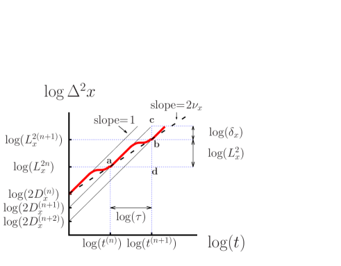
Figure 3: (Color online) Schematic of the mean-square displacement in the x direction, as a function of the time, shown by the red (tick) curve. The length of the segment bc is $\log_{10}(2D^{(n)}_{x})-\log_{10}(2D^{(n+1)}_{x})=\log_{10}(\delta_{x})$, because of Eq.(5). From the slopes ($=1$) of the full straight lines (representing the normal diffusion behaviors, $\Delta^{2}x=2D^{(n)}_{x}t$), one gets that the segments ad and cd have the same length or, equivalently, that $\log_{10}(\tau)=\log_{10}(L^{2}_{x})+\log_{10}(\delta_{x})$. The dashed straight line represents the global power law $\Delta^{2}x\sim t^{2\nu_{x}}$ with $2\nu_{x}=\log_{10}L^{2}_{x}/\log_{10}\tau$. Thus, $\nu_{x}=(2+\log_{10}\delta_{x}/\log_{10}L_{x})^{-1}$. The mean-square displacement in the y direction exhibits an analogous behavior.

Let us now consider a RW on the full self-affine structure. For a time $t$ in the interval $[t^{(n)},t^{(n+1)}]$, the following relations hold

$$L^{n}_{x}\lesssim\sqrt{\Delta^{2}x(t)}\lesssim L^{n+1}_{x},$$ (10)

$$L^{n}_{y}\lesssim\sqrt{\Delta^{2}y(t)}\lesssim L^{n+1}_{y},$$ (11)

and it will be impossible for the RW to distinguish the full self-affine structure from the nth-generation one. Thus, Eqs. (1) and (2) account for the RW behavior in that time window, and the mean-square displacement should behave qualitatively as sketched in Fig. 3. This behavior is reminiscent of single particle diffusion on a self-similar substrate, whose mean-square displacement as a function of time obeys a log-periodic modulated power-law lore2 . Because of the lack of symmetry between the $x$ and the $y$ directions, to describe diffusive behavior in the case of a self-affine substrate, we need not one but two functions, which we expect to be

$$\Delta^{2}x(t)=C_{x}t^{2\nu_{x}}f_{x}(t)$$ (12)

and

$$\Delta^{2}y(t)=C_{y}t^{2\nu_{y}}f_{y}(t),$$ (13)

where $C_{x}$ and $C_{y}$ are constants, $\nu_{x}$ and $\nu_{y}$ are the RW exponents, and $f_{x}(t)$ ($f_{y}(t)$) is a log-periodic function with period $\tau_{x}$ ($\tau_{y}$).

The values of these quantities can be computed from the parameters of the model, after simple geometrical analysis of Fig. 3 (see figure caption and Refs. lore2 ; lore1 for further details). The results are

$$\nu_{x}=\frac{1}{2+\frac{\log_{10}\delta_{x}}{\log_{10}L_{x}}}\;\;\;,$$ (14)

$$\nu_{y}=\frac{1}{2+\frac{\log_{10}\delta_{y}}{\log_{10}L_{y}}}\;\;\;,$$ (15)

$$\tau_{x}=\delta_{x}L_{x}^{2}$$ (16)

and

$$\tau_{y}=\delta_{y}L_{y}^{2}.$$ (17)

Note that, even when $\nu_{x}\neq\nu_{y}$, the period of the modulations coincide, because of the constraint (6), i.e.,

$$\tau_{x}=\delta_{x}L_{x}^{2}=\frac{D_{x}^{(n)}}{D_{x}^{(n+1)}}L_{x}^{2}=\frac{D_{y}^{(n)}}{D_{y}^{(n+1)}}L_{y}^{2}=\delta_{y}L_{y}^{2}=\tau_{y},$$ (18)

where we have also used (5) and (8). We call $\tau$ this period. From the equations above, the values of the period and the exponents are $\tau=35$, $\nu_{x}=0.4527$ and $\nu_{y}=0.3090$.

Let us note that the average time to escape from a unit cell of the nth-generation is $t^{(n)}=\tau^{n}$, which means that the relations (10) and (11) hold for,

$$\tau^{n}\lesssim t\lesssim\tau^{n+1}.$$ (19)

Then, when the RW leaves the initial region, of size $L^{n}_{x}\times L^{n}_{y}$, to enter the next one, of size $L^{n+1}_{x}\times L^{n+1}_{y}$, the length-width ratio ($L^{n}_{x}/L^{n}_{y}$) is increased by an anisotropic factor $a=L_{x}/L_{y}$, while the average time increases from $t$ to $\tau t$. On the other hand, according to (12) and (14), the corresponding mean square displacements are related by $\Delta^{2}x(\tau t)=L^{2}_{x}\Delta^{2}x(t)$ and $\Delta^{2}y(\tau t)=L^{2}_{y}\Delta^{2}y(t)$. Therefore, in this transition, the ratio $\sqrt{\Delta^{2}x/\Delta^{2}y}$ is also increased by a factor $a$; i.e., the space explored by the RW grows with the same anisotropy as the substrate where the diffusion takes place.

II.2 Model II

For this model, the unit cells for the zeroth, first and second generation are shown in Fig. 4. The full self-affine substrate is here also obtained when the generation order goes to infinity. The linear sizes of the nth-generation unit cell are $L^{n}_{x}$ and $L^{n}_{y}$, with $L_{x}=3$ and $L_{y}=2$.

Figure 4: The unit cells of model II. The zeroth, first, and second generations are shown in (a), (b), and (c), respectively. $L_{x}=3$ and $L_{y}=2$.

The diffusion of a single particle is analyzed as on model I. That is, we reformulate the two-dimensional RW problem on a one-dimensional array and compute the diffusion coefficients following the steady-state method celso .

For the $n$th generation, we obtain

$$D^{(n)}_{x}=(\frac{3}{4})^{n}k^{(0)},\;\;\;\mbox{for}\;n=0,1,2,...\;,$$ (20)

and thus,

$$D^{(n)}_{x}/D^{(n+1)}_{x}=\delta_{x}=4/3,\;\;\;\mbox{for}\;n=0,1,2,...\;.$$ (21)

In average, the time to leave a $n$th-generation unit cell along the $x$ direction becomes the same as that along the $y$ direction if

$$D^{(n)}_{y}=\frac{k^{(0)}}{3^{n}},\;\;\;\mbox{for}\;n=0,1,2,...\;,$$ (22)

which implies

$$D^{(n)}_{y}/D^{(n+1)}_{y}=\delta_{y}=3,\;\;\;\mbox{for}\;n=0,1,2,...\;.$$ (23)

The $k^{(i)}$’s, coming from (22), are again computed from (9) (with $L_{x}=3$ and $L_{y}=2$). Furthermore, in spite of the differences between model I and model II, the qualitative behavior sketched in Fig. 3 we expect to be valid for both models. Therefore, the RW exponents $\nu_{x}$ and $\nu_{y}$, and the period $\tau$ are given by (14), (15) and (18); with the values $\nu_{x}=0.4421$, $\nu_{y}=0.2789$ and $\tau=12$.

III Numerical Results

To test the predictions outlined above, we perform standard RW Monte Carlo simulations, on a nth-generation unit cell for each model. In model I (II) every RW starts at the center of symmetry of the cell (at the top-left most site). The value of n is always chosen large enough to prevent the RWs from reaching the cell borders (the bottom and right cell borders) during the simulation. Working on this cell is thus equivalent to working with the full self-affine structure. In all simulations the hopping rate $k^{(0)}$ is set to $1/4$, and the other $k^{(i)}$’s ($i\geq 1$) are obtained from (9). After every Monte Carlo step, the time is increased by $\Delta t=1$

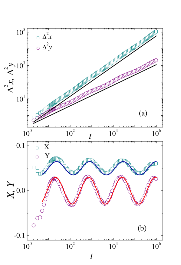
Figure 5: (Color online) (a): The mean-square displacements $\Delta^{2}x$ (green squares), and $\Delta^{2}y$ (purple circles) as functions of time for Model I. The upper straight line has a slope $2\nu_{x}$, with $\nu_{x}=0.4527$ obtained from Eq. (14). The lower straight line has a slope $2\nu_{y}$, with $\nu_{y}=0.3090$ obtained from Eq. (15). (b): $X=\log_{10}(\Delta^{2}x/A_{x}t^{2\nu_{x}})$ vs. $\log_{10}t$ ($Y=\log_{10}(\Delta^{2}y/A_{y}t^{2\nu_{y}})$ vs $\log_{10}(t)$) for the same data. $A_{x}$ and $A_{y}$ are a properly chosen constants. The curves represent the first-harmonic approximations $B_{x}\sin[2\pi\log_{10}(t)/\log_{10}(\tau)]+\alpha$ (blue-upper) and $B_{y}\sin[2\pi\log_{10}(t)/\log_{10}(\tau)]+\beta$ (red-lower). The period $\tau$ is given by Eq.(18). $B_{x}$, $B_{y}$, $\alpha$ and $\beta$ are fitted constants.

With the numerical results of model I, in Fig. 5-(a) we have plotted the mean-square displacement along the main directions. We see in these plots that both $\Delta^{2}x(t)$ and $\Delta^{2}y(t)$ are well described by modulated power laws. The upper and lower straight lines have slopes $2\nu_{x}$ and $2\nu_{y}$, respectively. They are drawn to guide the eyes, using the analytical values of the RW exponents. The log-periodicity of the modulations can be better observed in Fig. 5-(b), where we have plotted $\log_{10}(\Delta^{2}x/A_{x}t^{2\nu_{x}})$ and $\log_{10}(\Delta^{2}y/A_{y}t^{2\nu_{y}})$ against $\log_{10}(t)$, using the same data as in the part (a). $A_{x}$ ($A_{y}$) is a constant chosen to have the oscillations in the $x(y)$ direction centered around $0.00$ ($0.05$). The continuous lines are of the form $B\sin(2\pi\log_{10}(t)/\log_{10}(\tau)+\alpha)$, i.e., the first-harmonic approximation of a periodic function with period $\log_{10}(\tau)$, where $B$ and $\alpha$ are fitted parameters and $\tau=35$ (the above given analytical period). It is clear from this figure that the theoretical predictions (Eq.(14), (15) and (18)) are consistent with the numerical findings.

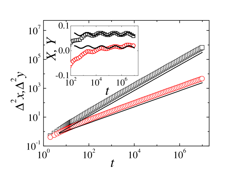
Figure 6: (Color online) The mean-square displacement $\Delta^{2}x$ (black squares) [$\Delta^{2}y$ (red circles)] versus time for model II. The top straight line has a slope $2\nu_{x}=0.8842$, and the lower straight line has a slope $2\nu_{y}=0.5579$. Both exponents are obtained from Eq.(14) and (15). The inset are plots of $X=\log_{10}\Delta^{2}x/A_{x}t^{2\nu_{x}}$ (black squares) and $Y=\log_{10}\Delta^{2}y/A_{x}t^{2\nu_{y}}$ (red circles) against $t$, for the same data. The curves were obtained as in Fig. 5, with the period $\tau$ calculated from Eq.(18).

The corresponding numerical results for model II are shown in Fig. 6. Note that, also for this model, at long times, the mean-square displacement as a function of time is well described by modulated power laws. To better appreciate the log-periodicity of the modulation, we have plotted $\log_{10}(\Delta^{2}x/A_{x}t^{2\nu_{x}})$ vs. $\log_{10}(t)$ and $\log_{10}(\Delta^{2}y/A_{y}t^{2\nu_{y}})$ vs $\log_{10}(t)$ in the inset of this figure. The fitting curves are of the form $D\sin(2\pi\log_{10}(t)/\log_{10}(\tau)+\alpha)$, with the analytical value $\tau=12$. The agreement between analytical and numerical results is also good.

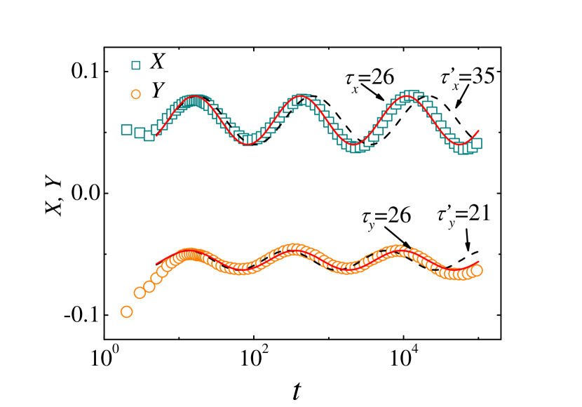
Figure 7: (Color online) Scaled mean-square displacements for Model III. Plot of $X=\log_{10}\Delta^{2}x/C_{x}t^{2\nu_{x}}$ vs. $\log_{10}t$ (green squares) and $Y=\log_{10}\Delta^{2}y/C_{y}t^{2\nu_{y}}$ vs. $\log_{10}t$ (orange circles), using numerical data ($C_{x}$ and $C_{y}$ are properly chosen constants, see the text). The full lines represent the first-harmonic approximations $A_{x}\sin(2\pi\log_{10}t)/\log_{10}(\tau)+\alpha)$ (upper) and $A_{y}\sin(2\pi\log_{10}t)/\log_{10}(\tau)+\beta)$ (lower) of $X$ and $Y$, respectively. Here, $\tau=26$, $A_{x}$, $A_{y}$, $\alpha$ and $\beta$ are fitted constants. The uppers dashed line represents the first-harmonic approximation of $X$, with period $\tau^{\prime}_{x}=35$. The lower dashed line represents the first-harmonic approximation of $Y$, with period $\tau^{\prime}_{y}=21$

We consider now a substrate (model III) which consists of the full self-affine structure of model I but with the same hopping rate $k^{(0)}$ between any pair of connected NN sites. For this model, the average time to leave a $n$-generation unit cell along the $x$ direction is different from that along the $y$ direction. It may occur that $L^{n}_{x}\lesssim\sqrt{\Delta^{2}x(t)}\lesssim L^{n+1}_{x}$, $L^{m}_{y}\lesssim\sqrt{\Delta^{2}y(t)}\lesssim L^{m+1}_{y}$, for a given time $t$ and $m\neq n$, which, in other words means that, near $t$, the RW behaves as in the $n$-generation substrate, regarding the $x$ direction, but as in the $m$-generation substrate, regarding the $y$ direction. Thus, we cannot expect the heuristic arguments in the previous section continue to be valid and we have then to study the problem numerically.

The logarithm of the scaled mean-squared displacements (in the x and y directions), i.e., $\Delta^{2}x/(A_{x}t^{2\nu_{x}})$ and $\Delta^{2}y/(A_{y}t^{2\nu_{y}})$ are plotted in Fig. 7 as a function of the logarithm of time. The RW exponents $\nu_{x}=0.4373$ and $\nu_{y}=0.3859$ in this figure are fitted values . Let us note that $\nu_{x}$ is different from $\nu_{y}$, and that the data of Fig. 7 strongly suggest that the modulation have the same period $\tau$ in both directions. As expected, the numerical values of these parameters are not in agreement with Eqs.(14), (15), and (18). We would like to remark that if we used Eqs.(14) and (15) (with $\delta_{x}=7/5$ and $\delta_{y}=7/3$ resulting from the new hopping rates) we would get the RW exponents $\nu^{\prime}_{x}=0.4527$ and $\nu^{\prime}_{y}=0.3609$, which, in turn would lead to the periods $\tau^{\prime}_{x}=L^{1/\nu^{\prime}_{x}}_{x}=35$ and $\tau^{\prime}_{y}=L^{1/\nu^{\prime}_{y}}_{y}=21$; different of each other (see caption of Fig. 3 for the equation $\tau=L^{1/\nu}$). Note that the numerical value of $\nu_{x}=0.4373$ ($\nu_{y}=0.3859$) is smaller than $\nu^{\prime}_{x}$ (larger than $\nu^{\prime}_{y}$), and the numerical value period $\tau$ is in the range $[\tau^{\prime}_{y},\tau^{\prime}_{x}]$ ($\tau\cong 26$). For model III, the Eqs. (10), (11) and (19) do not hold because, in average, the RW reaches the top or bottom border of the $n$-generation unit cell before reaching the right or left border of the same cell. In the case of model I, this is avoided by properly modifying some hopping rates in every generation. The diffusion spread in the $y$ direction is thus slowed down ($k^{(n)}<k^{(n-1)}$, see Eq.(9)), and the horizontal and vertical cell borders are, in average, simultaneously reached.

IV Conclusions and discussion

We have studied the problem of single particle diffusion on a finitely ramified self-affine structure in two dimensions. For a special kind of models, for which the ratio between the $x$ and $y$ mean-square displacements matches the structure anisotropy, we argue that the RW exponent in the x direction $\nu_{x}$ is different from that in the y direction $\nu_{y}$, and that the global subdiffusive behavior is modulated by log-periodic oscillations with a period $\tau$ which does not depend on the direction. The arguments employed in this work allow the main properties of the particle mean-square displacement to be obtained as a function of model parameters. Because our arguments are somehow heuristic, MC simulations using two models, I and II, were also carried out. The numerical results confirm our theoretical predictions.

For the rest of the self-similar systems, our conclusions are more limited, due to the lack of suitable analytical methods and that the RW explores the space with an anisotropy different from that of the substrate. The results of the MC simulations performed using one of these models (III), show (within the accuracy of the simulation) that, also in this case $\nu_{x}\neq\nu_{y}$ and the RW mean-square displacement is modulated by log-periodic oscillations with an isotropic period. However, we cannot guarantee that this behavior will hold in the limit of an arbitrary long time; that is why we have introduced models I and II. Let us finally note that the extension of our analytical results to other values of $L_{x}$ and $L_{y}$ is straightforward.

ACKNOWLEDGMENTS

This work was supported by the Universidad Nacional de Mar del Plata and the Consejo Nacional de Investigaciones Científicas y Técnicas-CONICET-(PIP 0041/2010-2012).

References

- (1) S. Alexander and R. Orbach, J. Phys. (France) Lett. 43, L625 (1982); R. Rammal and G. Toulouse, J. Phys. (France) Lett. 44, L13 (1983); D. Ben Avraham and S. Havlin, Diffusion and Reactions in Fractals and Disordered Media, Cambridge University Press, Cambridge (2000); S. Havlin and D. Ben-Avraham, Adv. Phys. 36, 695 (1987); J-P. Bouchaud and A. Georges. Phys. Rep. 195, 127 (1990).
- (2) W. Woess, Random Walks on Infinite Graphs and Groups, Cambridge UP (2000); P. J. Grabner and W. Woess, Stochastic Process. Appl. 69, 127 (1997); B. Krön and E. Teufl, Trans. Amer. Math. Soc. 356, 393 (2003); L. Acedo, S. B. Yuste, Phys. Rev. E 63, 011105 (2000); M. A. Bab, G. Fabricius and E. V. Albano, Europhys. Lett. 81, 10003 (2008); M. A. Bab, G. Fabricius and E. V. Albano, J. Chem. Phys. 128, 044911 (2008); A. L. Maltz, G. Fabricius, M. A. Bab and E. V. Albano, J. Phys. A: Math. Theor. 41, 495004 (2008); S. Weber, J. Klafter, A. Blumen, Phys. Rev. E 82, 051129 (2010).
- (3) L. Padilla, H. O. Mártin and J. L. Iguain, EPL 85, 20008 (2009).
- (4) L. Padilla, H. O. Mártin and J. L. Iguain, Phys. Rev. E. 82, 011124 (2010).
- (5) J. Bernasconi, W. R. Schneider, J. Stat. Phys 30, 355 (1983); D. Stauffer and D. Sornette, Physica A 252, 271 (1998); D. Stauffer, Physica A 266, 35 (1999) Zhang Yu-Xia, Sang Jian-Ping, Zou Xian-Wu, Jin Zhun-Zhi, Physica A 350, 163 (2005).
- (6) Y. Huang, H. Saleur, C. Sammis and D. Sornette, Europhys. Lett. 41, 43 (1998); H. Saleur, C. Sammis, D. Sornette, Geogphys. Res. 101, 17661 (1996).
- (7) A. Krawiecki, K. Kacperski, S. Matyjaśkiewicz, J. A. Hołyst, Chaos, Solitons and Fractals, 18, 89 (2003).
- (8) B. Kutnjak-Urbanc, S. Zapperi, S. Milosevic, H. E. Stanley Phys. Rev. E 54, 272 (1996); R. F. S. Andrade, Phys. Rev. E 61, 7196 (2000); M. A. Bab, G. Fabricius, E. V. Albano Phys. Rev. E 71, 036139 (2005); H. Saleur and D. Sornette, J. Phys. I (France) 6, 327 (1996).
- (9) D. Sornette, A. Johansen, A. Arneodo, J. F. Muzy, H. Saleur, Phys. Rev. Lett 76, 251 (1996).
- (10) Y. Huang, G. Ouillon, H. Saleur, D. Sornette, Phys. Rev. E 55, 6433 (1997).
- (11) D. Sornette, A. Johansen and J-P. Bouchaud, J. Phys. I (France) 6, 167 (1996); N. Vanderwalle, Ph. Boveroux, A. Minguet, M. Ausloos, Physica A 255, 201 (1998); N. Vanderwalle, M. Ausloos, Eur. J. Phys. B 4, 139 (1998); N. Vanderwalle, M. Ausloos, Ph. Boveroux, A. Minguet, Eur. J. Phys. B 9, 355 (1999).
- (12) B. Doucot, W. Wang, J. Chaussy, B. Pannetier, R. Rammal, A. Vareille, D. Henry, Phys. Rev. Lett. 57, 1235 (1986).
- (13) D. Sornette, Phys. Rep. 297, 239 (1998).
- (14) P. Meakin, Fractals, scaling and growth far from equilibrium, Cambridge UP (1998).
- (15) C. M. Aldao, J. L. Iguain and H. O. Mártin, Surf. Sci 366, 483 (1996).