Stepwise introduction of model complexity in a generalized master equation approach to time-dependent transport

Abstract

We demonstrate that with a stepwise introduction of complexity to a model of an electron system embedded in a photonic cavity and a carefully controlled stepwise truncation of the ensuing many-body space it is possible to describe the time-dependent transport of electrons through the system with a non-Markovian generalized quantum master equation. We show how this approach retains effects of an external magnetic field and the geometry of an anisotropic electronic system. The Coulomb interaction between the electrons and the full electromagnetic coupling between the electrons and the photons are treated in a non-perturbative way using “exact numerical diagonalization”.

I Introduction

Advances in techniques constructing and experimenting with quantum electrodynamic circuits have resulted in systems with very strong electron-photon coupling Niemczyk10:772 ; Frey11:01 ; Delbecq11:01 . Traditionally, some version of the Jaynes-Cummings model Jaynes63:89 is used to describe the energy spectrum of the closed system or its time evolution Amitabh93:2276 . Recently, we have shown that for a strong electron-photon coupling in a semiconductor nanostructure the Jaynes-Cumming model may not be adequate and one may have to consider a model with more than two electron levels and the diamagnetic term in the coupling Jonasson2011:01 . In continuation we have used our experience with describing the dynamics of open systems in terms of the generalized master equation (GME) Moldoveanu10:155442 ; Gudmundsson10:205319 to start the exploration of time-dependent transport properties of circuit quantum electrodynamic (circuit-QED) systems Gudmundsson12:1109.4728 .

Here, we will describe our approach with a special emphasis on what we call: “A stepwise introduction of complexity to a model and a carefully controlled stepwise truncation of the ensuing many-body space”. We will discuss technical issues that are common to models of different phenomena and fields, but we will use the model of Coulomb interacting electrons in a photonic cavity as an example to display our approach and findings.

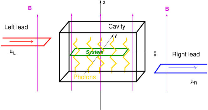
Figure 1: A schematic view of the total system consisting of a finite quantum wire (green, the central electronic system) in a photon cavity (bold black), coupled to external left (red) and right (blue) leads at different chemical potentials, $\mu_{\mathrm{L}}$ and $\mu_{\mathrm{R}}$. An external homogeneous magnetic field $\mathbf{B}$ (magenta) is perpendicular to the system and the leads. The lengths are not shown to scale. The length of the central system is 300 nm, but the characteristic lengths of the cavity are on the millimeter scale. The GaAs leads and central system contain a quasi-one-dimensional (Q1D) electron gas in 1 to 4 subbands of width 60 to 120 nm for the parameters to be introduced below. The cavity photon modes (yellow) are standing waves in the $z$-direction with an electric component in the $x$- or $y$-direction. The applied bias between the left and right leads is indicated by placing them at different levels with respect to the central system.

II The model of the closed system

The closed electron-photon system is a finite quasi-one-dimensional (Q1D) quantum wire placed in the center of a rectangular photon cavity (see Figure 1). It is described by the Hamiltonian Gudmundsson12:1109.4728

$$H {}_{0}=\sum_{i}E_{i}d_{i}^{\dagger}d_{i}+\hbar\omega a^{\dagger}a+\frac{1}{2}\sum_{ijrs}\langle ij|V_{\mathrm{Coul}}|rs\rangle d_{i}^{\dagger}d_{j}^{\dagger}d_{s}d_{r}$$

$$+{\cal E}_{\mathrm{c}}\sum_{ij}d_{i}^{\dagger}d_{j}\;g_{ij}\left\{a+a^{\dagger}\right\}$$ (1)

$$+{\cal E}_{\mathrm{c}}\left(\frac{{\cal E}_{\mathrm{c}}}{\hbar\Omega_{w}}\right)\sum_{i}d_{i}^{\dagger}d_{i}\left\{\left(a^{\dagger}a+\frac{1}{2}\right)+\frac{1}{2}\left(aa+a^{\dagger}a^{\dagger}\right)\right\}{},$$

where $E_{i}$ is the single-electron spectrum for the finite quantum wire with hard walls at $x=\pm L_{x}/2$ and parabolic confinement in the $y$-direction with characteristic energy $\hbar\Omega_{0}$. A static classical external magnetic field $\mathbf{B}=\mathbf{\nabla}\times\mathbf{A}_{\mathrm{ext}}=B\hat{\mathbf{z}}$ renormalizes the frequency of the $y$-confinement $\Omega_{w}^{2}=\omega_{c}^{2}+\Omega_{0}^{2}$ and the natural length scale $a_{w}=\sqrt{\hbar/(m^{*}\Omega_{w})}$ with the cyclotron frequency $\omega_{c}=eB/(m^{*}c)$. $d_{i}$ is an annihilation operator of the non-interacting single-electron state (SES) $|i\rangle$ with energy $E_{i}$, and $a$ is the annihilation operator for the single-photon mode with energy $\hbar\omega$. The kernel for the Coulomb interaction of the electrons is

$$V_{\mathrm{Coul}}(\mathbf{r}-\mathbf{r}^{\prime})=\frac{e^{2}}{\kappa\sqrt{(x-x^{\prime})^{2}+(y-y^{\prime})^{2}+\eta^{2}}},$$ (2)

with the small regularization factor selected such that $\eta/a_{w}\approx 7.1\times 10^{-3}$ when $a_{w}\approx 33.5$ nm at $B=0.1$ T for GaAs parameters, i. e. the effective mass $m^{*}=0.067m_{e}$, and the dielectric constant $\kappa=12.4$. The second line in the Hamiltonian (1) is the paramagnetic interaction between electrons and photons $(-\int d{\mathbf{r}}\;\mathbf{j}\cdot\mathbf{A})/c$, and the last line stems from the diamagnetic term in the interaction $(-e\int d{\mathbf{r}}\;\rho A^{2})/(2m^{*}c^{2})$. In terms of the field operators the charge current density and charge density are, respectively,

$$\mathbf{j}=-\frac{e}{2m^{*}}\left\{\psi^{\dagger}\left({\bm{\pi}}\psi\right)+\left({\bm{\pi}}^{*}\psi^{\dagger}\right)\psi\right\},$$ (3)

and

$$\rho=-e\psi^{\dagger}\psi,$$ (4)

where

$${\bm{\pi}}=\left(\mathbf{p}+\frac{e}{c}\mathbf{A}_{\mathrm{ext}}\right).$$ (5)

The photon cavity is assumed to be a rectangular box $(x,y,z)\in\{[-a_{\mathrm{c}}/2,a_{\mathrm{c}}/2]\times[-a_{\mathrm{c}}/2,a_{\mathrm{c}}/2]\times[-d_{\mathrm{c}}/2,d_{\mathrm{c}}/2]\}$ with the finite quantum wire centered in the $z=0$ plane. In the Coulomb gauge the polarization of the electric field can be chosen parallel to the transport in the $x$-direction by selecting the TE₀₁₁ mode, or perpendicular to it by selecting the TE₁₀₁ mode

$$\mathbf{A}(\mathbf{r})=\left({\hat{\mathbf{e}}_{x}\atop\hat{\mathbf{e}}_{y}}\right){\cal A}\left\{a+a^{\dagger}\right\}\left({\cos{\left(\frac{\pi y}{a_{\mathrm{c}}}\right)}\atop\cos{\left(\frac{\pi x}{a_{\mathrm{c}}}\right)}}\right)\cos{\left(\frac{\pi z}{d_{\mathrm{c}}}\right)},\quad\quad{\mbox{TE${}_{011}$}\atop\mbox{TE${}_{101}$}}.$$ (6)

${\cal A}$ is the amplitude of the cavity vector field defining a characteristic energy scale ${\cal E}_{\mathrm{c}}=e{\cal A}\Omega_{w}a_{w}/c=g^{\mathrm{EM}}$ for the electron-photon interaction and leaving an effective dimensionless coupling tensor

$$g_{ij}=\frac{a_{w}}{2\hbar}\int d{\mathbf{r}}\;[\psi_{i}^{*}(\mathbf{r})\left\{\left(\hat{\mathbf{e}}\cdot\bm{\pi}\right)\psi_{j}(\mathbf{r})\right\}+\left\{\left(\hat{\mathbf{e}}\cdot\bm{\pi}\right)\psi_{i}(\mathbf{r})\right\}^{*}\psi_{j}(\mathbf{r})],$$ (7)

defining the coupling of individual single-electron states $|i\rangle$ and $|j\rangle$ to the photonic mode. In the calculations of the energy spectrum of the Hamiltonian (1) we will retain all resonant and antiresonant terms in the photon creation and annihilation operators so we will not use the rotating wave approximation, but in the calculations of the electron-photon coupling tensor (7) we assume $a_{w},L_{x}<<a_{\mathrm{c}}$ and approximate $\cos(\pi\{x,y\}/a_{\mathrm{c}})~{}\sim 1$ in Eq. (6) for the cavity vector field $\mathbf{A}$.

The energy spectrum and the states of the Hamiltonian for the closed electron-photon system have to be sought for an unspecified number of electrons as we want to open the system up for electrons from the leads later. We will be investigating systems with few electrons present in the finite quantum wire, but it is not a trivial task to construct an adequate many-body (MB) basis for the diagonalization of $H_{0}$ since in addition to geometrical and bias (set by the leads) considerations we have strong requirements set both by the Coulomb and the photon interaction. Our solution to this dilemma and a mean to keep a tight lid on the exponential growth of the size of the required many-body Fock space is to do the diagonalization in two steps.

First, we select the lowest $N_{\mathrm{SES}}$ single-electron states (SESs) of the finite quantum wire. These have been found by diagonalizing the Hamiltonian operator for a single electron in the Q1D confinement and in a perpendicular constant magnetic field in a large basis of oscillator-like wave functions. Originally, we constructed a many-electron Fock space with $N_{\mathrm{MES}}=2^{N_{\mathrm{SES}}}$ states $|\mu\rangle$ Moldoveanu09:073019 ; Gudmundsson09:113007 . (We use Latin indices for the single-electron states and Greek ones for the many-electron states). This “simple binary” construction for the Fock-space does not deliver the optimal ratio of single-, two-, and higher number-of-electrons states for an interacting system when their energy is compared. Usually one ends up with too few SESs compared to the MESs. Here we will select 18 SESs and construct all possible combinations of 2-4 electron states. This can be refined further. These MESs, which are in fact Slater determinants, and which we denote as $|\mu\rangle$ (with an angular right bracket) are then used to diagonalize the part of the Hamiltonian (1) for the Coulomb interacting electrons only, supplying their spectrum ${\tilde{E}}_{\mu}$ and states $|\mu)$ (denoted now with a rounded right bracket). The eigenvectors from the diagonalization procedure define the unitary transform between the two sets of MESs, $|\mu)=\sum_{\alpha}{\cal V}_{\mu\alpha}|\alpha\rangle$. As the action of the creation and annihilation operators is only known in the non-interacting electron basis $\{|\mu\rangle\}$ we need this transform to write $H_{0}$ in the new Coulomb interacting basis $\{|\mu)\}$

$$H_{0} =\sum_{\mu}|\mu)\tilde{E}_{\mu}(\mu|+\hbar\omega a^{\dagger}a+{\cal E}_{\mathrm{c}}\sum_{\mu\nu ij}|\mu)\langle\mu|{\cal V}^{+}d_{i}^{\dagger}d_{j}{\cal V}|\nu\rangle(\nu|\;g_{ij}\left\{a+a^{\dagger}\right\}$$

$$+{\cal E}_{\mathrm{c}}\left(\frac{{\cal E}_{\mathrm{c}}}{\hbar\Omega_{w}}\right)\sum_{\mu\nu i}|\mu)\langle\mu|{\cal V}^{+}d_{i}^{\dagger}d_{i}{\cal V}|\nu\rangle(\nu|\left\{\left(a^{\dagger}a+\frac{1}{2}\right)+\frac{1}{2}\left(aa+a^{\dagger}a^{\dagger}\right)\right\}.$$ (8)

In order to finally obtain the energy spectrum of the electron-photon Hamiltonian (8) we need to construct a MB-space $|\mu)\otimes|N_{\mathrm{ph}}\rangle\longrightarrow|\mu\rangle_{\mathrm{e-EM}}$ out of the Coulomb interacting MESs $|\mu)$ and the eigenstates of the photon number operator $|N_{\mathrm{ph}}\rangle$. To properly take account of the effects of the Coulomb interaction we selected a large basis $\{|\mu\rangle\}$ and many photon states since the strong coupling to the cavity photons requires many states. For the system parameters to be introduced later we find that basis build up of the 64 lowest in energy Coulomb interacting MESs and 27 photon states is adequate for the transport bias windows and the electron-photon coupling to be selected later. The catch is that the unitary transform has to be performed with the full untruncated basis since ${\cal V}$ can not be truncated. In other words each of the 64 interacting MESs $|\mu)$ remains a superposition of all of the $2^{N_{\mathrm{SES}}}$ noninteracting MESs $|\mu\rangle$ with the same number of electrons $N_{\mathrm{e}}$, i. e. $|\mu)$ is a linear combination of a subset of $\binom{N_{\mathrm{SES}}}{N_{\mathrm{e}}}$ terms. (A similar issue is met when the dimensionless coupling tensor $g_{ij}$ (7) is transformed from the original single-electron basis to the single-electron states $|i\rangle$).

The diagonalization of $H_{0}$ produces the new interacting electron-photon states $|\breve{\mu})=\sum_{\alpha}{\cal W}_{\mu\alpha}|\alpha\rangle_{\mathrm{e-EM}}$ with a known integer electron content, but an indefinite number of photons, since the photon number operator does not commute with $H_{0}$.

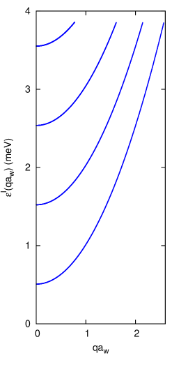
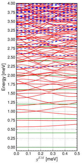
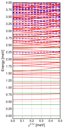
Figure 2: The single-electron energy spectrum of the leads (left panel) versus the “subband momentum” $qa_{w}$, and the many-body energy spectra for Coulomb interacting electrons coupled to quantized cavity photon modes with the electric component polarized along the finite quantum wire (x-polarization, center panel), and perpendicular to the wire (y-polarization, right panel) versus the electron-photon coupling strength $g^{\mathrm{EM}}={\cal E}_{\mathrm{c}}$. In the energy range shown there are states with no electrons (horizontal solid green), one electron (solid red), and two electrons (dashed blue). In order to reach convergence for high ${\cal E}_{\mathrm{c}}$ in this figure we use $N_{\mathrm{SES}}=200$ here. $B=0.1$ T, $\hbar\Omega_{0}=1.0$ meV, $\hbar\omega=0.4$ meV, $\hbar\Omega_{0}^{l}=1.0$ meV, $L_{x}=300$ nm, $m^{*}=0.067m_{e}$, $\kappa=12.4$, the dielectric constant of GaAs.

The MB energy spectra for the $x$- and $y$-polarization of the photon mode are shown in Fig. 2 in comparison with the subbandstructure of the single-electron spectrum of the leads. The difference in the energy spectra for the $x$- and the $y$-polarization stems from the anisotropic electron system. The photon mode selected with energy $0.4$ meV is close to be in resonance with the motion in the $x$-direction, but quite far from the fundamental energy in the $y$-direction, $1.0$ meV. The spectrum for the $x$-polarization thus displays stronger dispersion and interaction of levels than the spectrum for the $y$-polarization.

The states of the closed system in Fig. 2 have a definite number of electrons and an undetermined number of photons of one given polarization. Later when the system is coupled to the leads one can expect the electrons entering the system to radiate photons with any polarization. A preferred polarization could though be influenced by the aspect ratio of the cavity. In the treatment of the time-dependent system to follow we assume the electrons only to radiate photons with one given polarization. This is done to facilitate the numerical calculations and the analysis of a system with a strong spatial anisotropy.

III Opening of the system, coupling to external leads

At time $t=0$ the closed system of Coulomb interacting electrons coupled to cavity photons described by the Hamiltonian (8) is connected to two external semi-infinite quasi-one-dimensional quantum wires in a perpendicular magnetic field Gudmundsson10:205319 . We use an approach introduced by Nakajima and Zwanzig to project the time evolution of the total system onto the central system by partial tracing operations with respect to the operators of the leads Nakajima58:948 ; Zwanzig60:1338 . The coupling Hamiltonian of the central system (i. e. the short Q1D wire) to the leads is of the form

$$H_{\mathrm{T}}(t)=\sum_{i,l}\chi^{l}(t)\int dq\;\left\{T^{l}_{qi}c_{ql}^{\dagger}d_{i}+(T^{l}_{qi})^{*}d_{i}^{\dagger}c_{ql}\right\},$$ (9)

where $l\in\{L,R\}$ refers to the left or the right lead, and $\chi^{l}(t)$ is the time-dependent switching function of the coupling. The operators $c_{ql}$ and $c_{ql}^{\dagger}$ annihilate and create an electron in the $l$-lead with a quantum number $q$ referring both to the continuous momentum $q$ and the subband $n^{l}$, see Fig. 2 for the corresponding energy spectrum. To represent the geometry of the leads and the central system, the coupling tensor $T^{l}_{qi}$ of single-electron states $|q\rangle$ in the lead $l$ to single-electron states states $|i\rangle$ in the system is modeled as a non-local overlap integral of the corresponding wave functions in the contact regions of the system, $\Omega_{S}^{l}$, and the lead $l$, $\Omega_{l}$Gudmundsson09:113007

$$T^{l}_{iq}=\int_{\Omega_{S}^{l}\times\Omega_{l}}d{\bf r}d{\bf r}^{\prime}\left[\psi^{l}_{q}({\bf r}^{\prime})\right]^{*}\psi^{S}_{i}({\bf r})\;g^{l}_{iq}({\bf r},{\bf r^{\prime}}).$$ (10)

The function

$$g^{l}_{iq}({\bf r},{\bf r^{\prime}})=g_{0}^{l}\exp{\left[-\delta_{1}^{l}(x-x^{\prime})^{2}-\delta_{2}^{l}(y-y^{\prime})^{2}\right]}\times\exp{\left(\frac{-|E_{i}-\epsilon^{l}(q)|}{\Delta_{E}^{l}}\right)}$$ (11)

with ${\bf r}\in\Omega_{\mathrm{S}}^{l}$ and ${\bf r}^{\prime}\in\Omega_{l}$ defines the ‘nonlocal Gaussian overlap’ determined by the constants $\delta_{1}$ and $\delta_{2}$, and the affinity of the states in energy $\Delta_{E}^{l}$. The energy spectra of the leads are represented by $\epsilon^{l}(q)$.

The time-evolution of the total system is determined by the Liouville-von Neumann equation

$$i\hbar\dot{W}(t)=[H(t),W(t)],\quad W(t<0)=\rho_{\mathrm{L}}\rho_{\mathrm{R}}\rho_{\mathrm{S}},$$ (12)

with $W$ the statistical operator of the total system and $\rho_{l}$ the equilibrium density operator of the disconnected lead $l\in\{L,R\}$ having chemical potential $\mu_{l}$

$$\rho_{l}=\frac{e^{-\beta(H_{l}-\mu_{l}N_{l})}}{{\rm Tr}_{l}\{e^{-\beta(H_{l}-\mu_{l}N_{l})}\}},$$ (13)

where $H_{l}$ is the Hamiltonian of the electrons in lead $l\in\{\mathrm{L,R}\}$ and $N_{l}$ is their number operator. The Liouville-von Neumann equation (12) is projected on the central system of coupled electrons and photons by a partial tracing operation with respect to the operators of the leads. Defining the reduced density operator (RDO) of the central system

$$\rho_{\mathrm{S}}(t)={\rm Tr}_{\mathrm{L}}{\rm Tr}_{\mathrm{R}}W(t),\quad\rho_{\mathrm{S}}(0)=\rho_{\mathrm{S}},$$ (14)

we obtain an integro-differential equation for the RDO, the generalized master equation (GME)

$$\dot{\rho}_{\mathrm{S}}(t)=-\frac{i}{\hbar}\left[H_{\mathrm{S}},{\rho}_{\mathrm{S}}(t)\right]-\frac{\mathrm{Tr}_{\mathrm{LR}}}{\hbar^{2}}\left\{\left[H_{\mathrm{T}}(t),\int_{0}^{t}dt^{\prime}\;\left[U(t-t^{\prime})H_{\mathrm{T}}(t^{\prime})U^{+}(t-t^{\prime}),\qquad\quad{\vphantom{.}}\right.\right.\right.$$

$$\left.\left.\left.U_{0}(t-t^{\prime})\rho_{\mathrm{S}}(t^{\prime})U_{0}^{+}(t-t^{\prime})\rho_{\mathrm{L}}\rho_{\mathrm{R}}\right]\vphantom{\sum}\right]\right\},$$ (15)

where the time evolution operator for the closed systems of Coulomb interacting electrons coupled to photons on one hand, and on the other hand noninteracting electrons in the leads is given by $U(t)=\exp{\{-i(H_{\mathrm{e}}+H_{\mathrm{Coul}}+H_{\mathrm{EM}}+H_{\mathrm{L}}+H_{\mathrm{R}})t/\hbar\}}$, without the coupling to the leads $H_{\mathrm{T}}(t)$. Here, $H_{\mathrm{e}}$ is the Hamiltonian for the electrons in the central system, $H_{\mathrm{Coul}}$ their mutual Coulomb interaction, $H_{\mathrm{EM}}$ is the Hamiltonian for the photons in the cavity together with their interaction to the electrons, and $H_{\mathrm{L,R}}$ are the Hamiltonian operators for the electrons in the left and right leads. The time evolution of the closed system of Coulomb interacting electrons interacting with the photons is governed by $U_{0}(t)=\exp{\{-iH_{0}t/\hbar\}}$. The GME (15) is valid in the weak system-leads coupling limit since we have only retained terms of second order in the coupling Hamiltonian $H_{\mathrm{T}}$ in its integral kernel. It should though be stressed that we are not approximating the GME to second order in the coupling as its integral structure effectively provides terms of any order, but with a structure reflecting the type of the integral kernel.

Commonly, the GME is written in terms of spectral densities for the states in the system instead of the coupling tensor (10). We do not make this transformation but the spectral densities for the 10 lowest SESs used in our system have been presented elsewhere Gudmundsson12:1109.4728 (Here the overall coupling is one quarter of the value used in Ref. Gudmundsson12:1109.4728 ). The spectral density is a particularly useful physical concept as it demonstrates the spectral broadening of the SESs in the finite system due to the coupling to the leads.

IV Transport characteristics

The time-dependent coupling betweeen the leads and the central system is modeled by the switching functions $\chi^{l}(t)$. These functions may be considered input elements of the transport problem: stepwise functions, periodic, relatively phase-shifted, etc. In the following examples the left and right leads are coupled simultaneously smoothly to the central system by use of the switching function

$$\chi^{l}(t)=\left(1-\frac{2}{e^{\alpha^{l}t}+1}\right),\quad l\in\{L,R\}$$ (16)

with $\alpha^{l}=0.3$ ps^-1. The temperature of the leads $T=0.5$ K, and the overall coupling strength $g_{0}^{l}a_{w}^{3/2}=13.3$ meV, is much lower than in our earlier calculation Gudmundsson12:1109.4728 . We choose $\delta_{1,2}^{l}a_{w}^{2}=0.4916$ meaning that states of a lead and the central system with considerable charge density within a length equivalent to $2a_{w}$ ($a_{w}\approx 33.5$ nm here) could be well coupled.

The energy of the photon mode is $\hbar\omega=0.4$ meV, and the electron confinement in the $y$-direction has the energy scale $\hbar\Omega_{0}=1.0$ meV. The energy separation of the lowest states for the motion in the $x$-direction is lower, $\sim 0.2$ meV. The Coulomb interaction has a characteristic energy scale $0.5e^{2}/(\kappa a_{w})\approx 1.7$ meV. The external magnetic field is low enough so that only the highest lying SESs show any effects of the Lorentz force. We expect thus the transport properties of the system to be anisotropic at a low energy scale with respect to polarization of the photon field along ($x$-direction) or perpendicular ($y$-direction) to the transport.

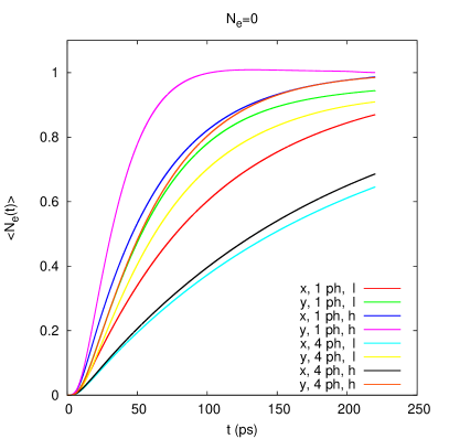
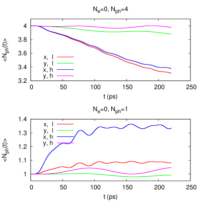
Figure 3: The total mean number of electrons $\langle N_{\mathrm{e}}(t)\rangle$ (left panel), and the total mean photon number $\langle N_{\mathrm{ph}}(t)\rangle$ (right panels) as a function of time, polarization of the photon field ($x$ or $y$) and bias window low (l: $\mu_{L}=2.0$ and $\mu_{R}=1.4$ meV) or high (h: $\mu_{L}=3.0$ and $\mu_{R}=2.5$ meV). $B=0.1$ T, $g^{\mathrm{EM}}=0.1$ meV, $\hbar\Omega_{0}=1.0$ meV, $L_{x}=300$ nm, $\hbar\omega=0.4$ meV, $\Delta^{l}_{E}=0.25$ meV, $g_{0}^{l}a_{w}^{3/2}=13.3$ meV, $\delta_{1,2}^{l}a_{w}^{2}=0.4916$, $m^{*}=0.067m_{e}$, and $\kappa=12.4$.

In the present calculations we start with a central system empty of electrons, but with one or four photons in the cavity. For $N_{\mathrm{SES}}=18$ the state with no electron, but one photon, is $|\breve{2})$ for both polarizations. The state containing 4 photons and no electrons is $|\breve{14})$ for the $x$-polarization and $|\breve{15})$ in the case of the $y$-polarization. The time evolution of the total mean electron number $\langle N_{\mathrm{e}}(t)\rangle$ is seen in the left panel of Fig. 3 and the total mean number of photons $\langle N_{\mathrm{ph}}(t)\rangle$ is displayed in the lower right panel for the case of initially one photon and in the upper panel for initially 4 photons. The charging of the system is in most cases fastest for the higher bias window as the active states of the central system are well coupled to states in the leads that carry a large current in this energy range. The presence of photons in the system sharply diminishes the charging speed, especially for their polarization along the transport direction ($x$-direction). The time evolution of the total mean number of photons in the system does not give much insight into what is happening in the system, but it is though clear that it varies more in case of the $x$-polarization.

Very similar information can be read from the graphs of the total currents in the left (L) or the right (R) leads shown in Fig. 4.

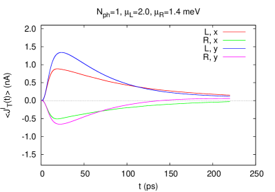
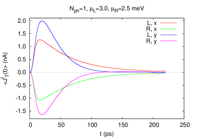
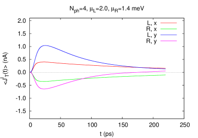
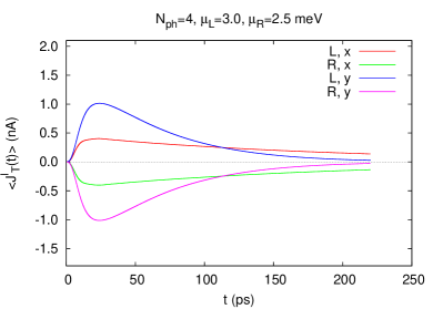
Figure 4: The total current from the left lead (L), and into the right lead (R) as a function of time for $g^{\mathrm{EM}}=0.1$ meV and polarization of the photon field ($x$ or $y$). Initially, at $t=0$ there is one photon in the cavity (top panel), or 4 photons (bottom panel). The bias window is low ($\mu_{L}=2.0$ and $\mu_{R}=1.4$ meV) for the left panels and high ($\mu_{L}=3.0$ and $\mu_{R}=2.5$ meV) for the right panels. $B=0.1$ T, $\hbar\Omega_{0}=1.0$ meV, $L_{x}=300$ nm, $\hbar\omega=0.4$ meV, $\mu_{L}=2.0$ meV, $\mu_{R}=1.4$ meV, $\Delta^{l}_{E}=0.25$ meV, $g_{0}^{l}a_{w}^{3/2}=13.3$ meV, $\delta_{1,2}^{l}a_{w}^{2}=0.4916$, $m^{*}=0.067m_{e}$, and $\kappa=12.4$.

The negative values for the current into the right lead indicate a flow from the lead to the central system. A note of caution here is that we are concentrating on the charging time-regime here and we are not trying to reach a possible steady state, but clearly we are most likely in a Coulomb blocking range. It is our experience that a considerable probability for two electrons in the system is only seen after several two-electron states are in or under the bias window. The reason for this is most likely the different coupling between states in the leads and the system, how far the system is from equilibrium and, and how the coupling strength influences the rate of occupation of various dynamically correlated states. We have verified that a still higher bias leads to a nonvanishing steady state current. Here, we always have at least one photon initially in the cavity and we notice that the charging rate and the currents are mostly higher for the $y$-polarization. The time-scale for the charging in the $x$-polarization gets very long as the photon number is increased from 1 to 4. This is not a total surprise since the energy of the photons is closer to characteristic excitation energies for a motion in the $x$-direction.

A detailed view of the charging processes can be obtained by observing the time-dependent probabilities for occupation of the available many-body states (MBS) by electrons or photons. In Fig. 5 we see the mean charge in the MBS for the transport through the lower bias window $\mu_{L}=2.0$ and $\mu_{R}=1.4$ meV.

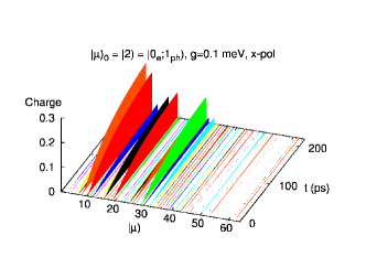
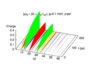
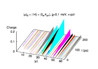
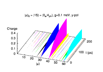
Figure 5: The mean number of electrons $\langle N_{\mathrm{e}}(t)\rangle$ in a MBS $|\breve{\mu})$ for a low bias window ($\mu_{L}=2.0$ and $\mu_{R}=1.4$ meV) for $x$-polarization (left) and $y$-polarization (right) as a function of time. Initially, at $t=0$, there is one photon in the cavity (top panels), or 4 photons (bottom panels). The initial number of electrons is zero in all cases. $B=0.1$ T, $g^{\mathrm{EM}}=0.10$ meV, $\hbar\omega=0.4$ meV, $\hbar\Omega_{0}=1.0$ meV, $\Delta^{l}_{E}=0.25$ meV, $g_{0}^{l}a_{w}^{3/2}=13.3$ meV, $\delta_{1,2}^{l}a_{w}^{2}=0.4916$, $L_{x}=300$ nm, $m^{*}=0.067m_{e}$, and $\kappa=12.4$.

The MBS $|\breve{\mu})$ are numbered according to increasing energy. We see clearly that the system is not close to equilibrium and the charge is “scattered” to more states for the $x$-polarization than the $y$-polarization. The presence of photons has large effects on the electrons in the system.

Very similar story can be said about the results for the higher bias window, $\mu_{L}=3.0$ and $\mu_{R}=2.5$ meV displayed in Fig. 6.

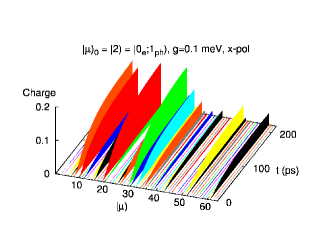
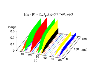
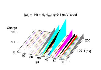
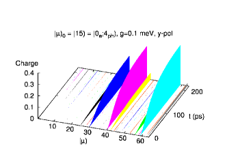
Figure 6: The mean number of electrons $\langle N_{\mathrm{e}}(t)\rangle$ in a MBS $|\breve{\mu})$ for a high bias window ($\mu_{L}=3.0$ and $\mu_{R}=2.5$ meV) for $x$-polarization (left) and $y$-polarization (right) as a function of time. Initially, at $t=0$, there is one photon in the cavity (top panels), or 4 photons (bottom panels). The initial number of electrons is zero in all cases. $B=0.1$ T, $g^{\mathrm{EM}}=0.10$ meV, $\hbar\omega=0.4$ meV, $\hbar\Omega_{0}=1.0$ meV, $\Delta^{l}_{E}=0.25$ meV, $g_{0}^{l}a_{w}^{3/2}=13.3$ meV, $\delta_{1,2}^{l}a_{w}^{2}=0.4916$, $L_{x}=300$ nm, $m^{*}=0.067m_{e}$, and $\kappa=12.4$.

Especially interesting is to see that the results for both polarizations are almost identical for the higher and lower bias window for the case of 4 photons initially in the central system. The effects of the bias window are washed out by the strong interaction with the quantized electromagnetic field in the cavity. We have though to bring in a note of caution here and admit that this effect should be studied further using a larger MB basis for the RDO.

A complete picture can not be reached without exploring the time-evolution of the mean photon number per MBS presented in Fig. 7 for the lower bias window and in 8 for the higher bias window.

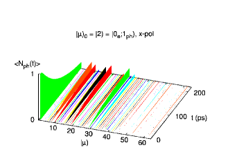
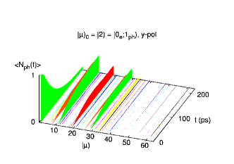
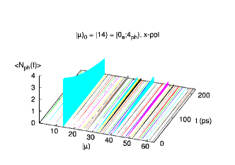
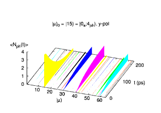
Figure 7: The mean number of photons $\langle N_{\mathrm{ph}}(t)\rangle$ in a MBS $|\breve{\mu})$ for a low bias window ($\mu_{L}=2.0$ and $\mu_{R}=1.4$ meV) for $x$-polarization (left) and $y$-polarization (right) as a function of time. Initially, at $t=0$, there is one photon in the cavity (top panels), or 4 photons (bottom panels). $B=0.1$ T, $g^{\mathrm{EM}}=0.1$ meV, $\hbar\omega=0.4$ meV, $\hbar\Omega_{0}=1.0$ meV, $\Delta^{l}_{E}=0.25$ meV, $g_{0}^{l}a_{w}^{3/2}=13.3$ meV, $\delta_{1,2}^{l}a_{w}^{2}=0.4916$, $L_{x}=300$ nm, $m^{*}=0.067m_{e}$, and $\kappa=12.4$.

Again we notice that the state of the system, the distribution of the photon component into various MBS, is almost independent of the the bias window in the case of 4 photons initially in the cavity.

But, here another very important fact about the system evolution becomes evident. The occupation of the initial photon state seems to vary much faster with time than the total mean number of photons shown in Fig. 3. The slow decay of the charging current in Fig. 4 for the system with 4 photons initially might also indicate that radiation processes here are slow. Why then do we have a fast redistribution of the photon component between the available MBS initially, during the switch-on process? The resolution of this dilemma comes from remembering the structure of the interaction terms. Part of the interaction is an integral over the term $\mathbf{j}\cdot\mathbf{A}$. We have a vector field initially present in the system. The high current into the system during the transient phase, when the contacts between the leads and the central system are switched on, creates a strong interaction that can “scatter” the electrons and the photons to different MBS, few or many, depending on selections rules and resonances. This initial rushing of electrons from both ends of the finite quantum wire is a longitudinal (irrotational) current that enhances the coupling to the photon field.

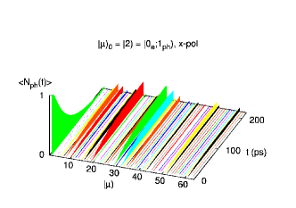
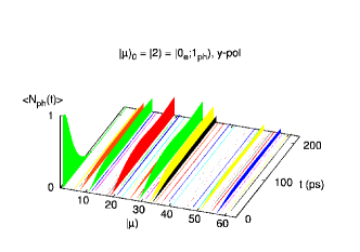
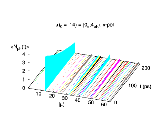
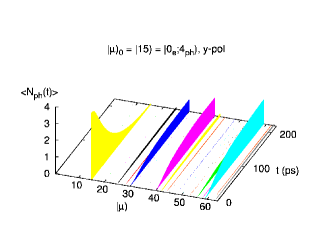
Figure 8: The mean number of photons $\langle N_{\mathrm{ph}}(t)\rangle$ in a MBS $|\breve{\mu})$ for a high bias window ($\mu_{L}=3.0$ and $\mu_{R}=2.5$ meV) for $x$-polarization (left) and $y$-polarization (right) as a function of time. Initially, at $t=0$, there is one photon in the cavity (top panels), or 4 photons (bottom panels). $B=0.1$ T, $g^{\mathrm{EM}}=0.1$ meV, $\hbar\omega=0.4$ meV, $\hbar\Omega_{0}=1.0$ meV, $\Delta^{l}_{E}=0.25$ meV, $g_{0}^{l}a_{w}^{3/2}=13.3$ meV, $\delta_{1,2}^{l}a_{w}^{2}=0.4916$, $L_{x}=300$ nm, $m^{*}=0.067m_{e}$, and $\kappa=12.4$.

This effect can be seen very well by comparing the photon distribution into the MBS at the low bias window and for the case of only one photon initially present in the cavity.

In case of the $x$-polarization we see that the system seems to develop a higher “impedance” acting against its charging as the number of photons is increased, and at the same time the electrons that enter the system are scattered to a wide range of MBS. The “impedance” has to be understood from the fact that the photon field is polarizing the electron density inside the system along the $x$-direction. Effectively, the states may gain coupling strength to the leads, but that works in both ways. The electrons enter the system easily and leave it equally easily at the same end before they can be transported through it. The charging of the system is counteracted by an effective scattering of a localized photon field. A phenomena that should be similar for a system with localized phonons.

V Summary

In this publication we have shown how we have successfully been able to implement a scheme which we wish to call: “A stepwise introduction of complexity to a model description and a careful counteracting stepwise truncation of the ensuing many-body space” to describe a time-dependent transport of Coulomb interacting electrons through a photon cavity. We have used this approach to demonstrate how the geometry of a particular system leaves its fingerprints on its transport properties. We guarantee geometrical dependence by using a phenomenological description of the system-lead coupling based on a nonlocal overlap of the single-electron states in the leads and the system in the contact area, and by using a large basis of SESs in order to build our MBS. The Coulomb interaction is implemented by an “exact numerical diagonalization”, and the coupling to the quantized electromagnetic cavity field of a single frequency is carried out using both the paramagnetic and the diamagnetic part of the charge current density. The coupling of the electrons and the photons is also treated by an exact numerical diagonalization without resorting to the rotating wave approximation. This approach is thus applicable for the modeling of circuit-QED elements in the strong coupling limit.

We have deployed the GME method to include memory effects without a Markov approximation. Moreover, the GME approach is utilized to describe the coupling of the electron-photon system to the external leads. At this moment in the development of the model we ignore the spin variable of freedom, but it can easily be included. The inclusion of the spin is (more or less) straight forward, but it requires a double amount of computer memory and an increased number of MBSs in the GME solver. This is work in progress now.

We concentrate our investigations on the charging regime of the system and find that it is strongly influenced by the presence of photons in the cavity, their polarization and the geometry of the system. We consider these results presented here as the mere initial steps into the exploration of a fascinating regime of circuit-QED elements.

For the numerical implementation we rely heavily on parallel processing, but we foresee further refinement in the truncation schemes for the many-body spaces and in the parallelization that will allow us to describe systems of increased complexity.

- (1) T. Niemczyk, F. Deppe, H. Huebl, E. P. Menzel, F. Hocke, M. J. Schwarz, J. J. Garcia-Ripoll, D. Zueco, T. Hümmer, E. Solano, A. Marx, and R. Gross, Nature Physics 6, 772 (2010).
- (2) T. Frey, P. J. Leek, M. Beck, A. Blais, T. Ihn, K. Ensslin, and A. Wallraff, arXiv:1108.5378 (2011).
- (3) M. Delbecq, V. Schmitt, F. Parmentier, N. Roch, J. Viennot, G. Fève, B. Huard, C. Mora, A. Cottet, and T. Kontos, Phys. Rev. Lett. 107, 256804 (2011).
- (4) E. T. Jaynes and F. W. Cummings, Proc. IEEE. 51, 89 (1963).
- (5) A. Joshi and S. V. Lawande, Phys. Rev. A 48, 2276 (1993).
- (6) O. Jonasson, C. S. Tang, H. S. Goan, A. Manolescu, and V. Gudmundsson, New Journal of Physics 14, 013036 (2012).
- (7) V. Moldoveanu, A. Manolescu, C. S. Tang, and V. Gudmundsson, Phys. Rev. B 81, 155442 (2010).
- (8) V. Gudmundsson, C. S. Tang, O. Jonasson, V. Moldoveanu, and A. Manolescu, Phys. Rev. B 81, 205319 (2010).
- (9) V. Gudmundsson, O. Jonasson, C. S. Tang, H. S. Goan, and A. Manolescu, Phys. Rev. B 85, 075306 (2012).
- (10) V. Moldoveanu, A. Manolescu, and V. Gudmundsson, New Journal of Physics 11(7), 073019 (2009).
- (11) V. Gudmundsson, C. Gainar, C. S. Tang, V. Moldoveanu, and A. Manolescu, New Journal of Physics 11(11), 113007 (2009).
- (12) S. Nakajima, Prog. Theor. Phys. 20, 948 (1958).
- (13) R. Zwanzig, J. Chem. Phys. 33, 1338 (1960).