Violent and mild relaxation of an isolated self-gravitating uniform and spherical cloud of particles

Abstract

The collapse of an isolated, uniform and spherical cloud of self-gravitating particles represents a paradigmatic example of a relaxation process leading to the formation of a quasi-stationary state in virial equilibrium. We consider several N-body simulations of such a system, with the initial velocity dispersion as a free parameter. We show that there is a clear difference between structures formed when the initial virial ratio is $b_{0}=2K_{0}/W_{0}<b_{0}^{c}\approx-1/2$ and $b_{0}>b_{0}^{c}$. These two sets of initial conditions give rise respectively to a mild and violent relaxation occurring in about the same time scale: however in the latter case the system contracts by a large factor, while in the former it approximately maintains its original size. Correspondingly the resulting quasi equilibrium state is characterized by a density profile decaying at large enough distances as $r^{-4}$ or with a sharp cut-off. The case $b_{0}<b_{0}^{c}$ can be well described by the Lynden-Bell theory of collisionless relaxation considering the system confined in a box. On the other hand the relevant feature for $b_{0}>b_{0}^{c}$ is the ejection of particles and energy, which is not captured by such a theoretical approach: for this case we introduce a simple physical model to explain the formation of the power-law density profile. This model shows that the behavior $n(r)\sim r^{-4}$ is the typical density profile that is obtained when the initial conditions are cold enough that mass and energy ejection occurs. In addition, we clarify the origin of the critical value of the initial virial ratio $b_{0}^{c}$.

1 Introduction

The evolution of a system of massive particles interacting solely by Newtonian gravity is a paradigmatic problem for astrophysics, cosmology and statistical physics. The underlying open question concerns the relaxation mechanism that drives the system to form structures which seem to be in a sort of equilibrium, as for instance different kind of astrophysical objects such as globular clusters, galaxies, and galaxy clusters (Lynden-Bell, 1967; Padmanabhan, 1990; Binney & Tremaine, 1994; Saslaw, 2000; Heggies, 2003; Aarseth, 2003). In a galaxy the two body relaxation time is of order $\tau_{2}\approx 10^{17}$ years (Binney & Tremaine, 1994), and is much longer than the age of the universe (i.e., $\approx 10^{10}$ years): for this reason these objects are not in thermal equilibrium. However, they present common features as the luminosity profiles (see e.g., de Vaucouleurs (1948); Binney & Merrifield (1998)). Much theoretical work has been devoted to study the dynamical model to characterize such profiles and despite the numerical simulations have shown that structures formed in some cases are compatible with observations, the physical origin of these profiles has not been yet clarified from a theoretical point of view. Namely, the problem still remains to explain how to form the shape of density profiles and of velocity distributions of stellar structures like elliptical galaxies and globular clusters that are generally characterized by a dense central core and a dilute halo — where the halo is often featured by a power-law decay of the radial density (Binney & Tremaine, 1994; Binney & Merrifield, 1998).

In cosmology one faces a different but somewhat related problem. Since more than a decade it has been realized that a major issue about gravitational clustering dynamics concerns the formation of the so-called halo-structures, which are considered the primary building blocks in terms of which the non-linear structures observed in cosmological simulations are described (Cooray & Sheth, 2002). These are approximately spherical symmetric structures, but sometimes with complex substructures, and with a density profile that that has almost universal statistical features and unknown dynamical origin. Density profiles of dark matter halos have become one of the most challenging issues for our understanding of cold dark matter structure formation. Numerical simulations provide evidences of steep central density cusps with power law slopes $\rho\sim r^{-\beta}$, with $\beta\approx 1$ at small scales and $\beta\approx 3$ at large ones (Navarro et al., 1996, 1997; Moore et al., 1988, 2001; Diemand etal., 2004; Reed etal., 2005; Navarro et al., 2004; Merritt et al., 2006). Recently Graham et al. (2006) showed that in simulated dark matter models, at large enough scales, slopes of $\beta\approx-4$ might be permitted. Several attempts have been made for an analytical derivation of the density profile (see, e.g., Bertschinger (1985); Syer & White (1998); Subramanian et al. (2000); Hiotelis (2002); Manrique etal. (2002); Dekel etal. (2003) and references therein), and none seem to present a clear and simple explanation for the findings of N-body codes.

The question of the nature of the equilibrium properties of these core-halo structures is thus relevant both in astrophysics and cosmology and thus one would like to develop a statistical mechanics approach to describe these systems. However, one must consider that, from the point of view of statistical physics, self-gravitating systems present fundamental problems, that are also common to other long-range interacting systems. Indeed, it is well known since the pioneering works of Boltzmann and Gibbs, that systems with a pair potential decaying with an exponent smaller than that of the embedding space, present several fundamental problems that prevent the use of equilibrium statistical mechanics: thermodynamic equilibrium is never reached and the laws of equilibrium thermodynamics do not apply (Padmanabhan, 1990; Dauxois et al., 2003; Campa et al., 2008). Rather these systems reach, driven by a mean-field collisionless relaxation dynamics, quasi-equilibrium configurations, or quasi-stationary state (QSS), whose lifetime diverge with the number of particles $N$ (Dauxois et al., 2003; Campa et al., 2008; Yamaguchi, 2008; Gabrielli et al., 2010; Joyce & Worrakitpoonpon, 2012; Worrakitpoonpon & Joyce, 2012). The formation of QSS is at present one of the most living subjects in non-equilibrium statistical physics and a general theoretical framework is still lacking: it is thus necessary to consider toy models and/or relatively simple systems that can be studied through numerical well-controlled experiments.

In order to understand the formation of a core-halo structure, a paradigmatic example is represented by the collapse of a spherical, isolated and uniform cloud of $N$ randomly placed particles with mass density $\rho_{0}$ interacting only by Newtonian gravity. This system has been considered since the early numerical studies (Hénon, 1964; van Albada, 1982) when it was realized that it relaxes violently, in a typical time scale $\tau_{D}=\sqrt{3\pi/(32G\rho_{0})}$, to produce a virialized state. Such a time scale is much shorter than the two-body collisional time scale $\tau_{2}\approx N/\log(N)\tau_{D}$ (Binney & Tremaine, 1994; Saslaw, 2000) and for this reason in the time range $\tau_{D}<t<\tau_{2}$ the system relaxes into a QSS in virial equilibrium. Then, because of two-body collisions particles can gain some kinetic energy and evaporate from the system: on a time scale of the order of $\tau_{2}$ the system changes shape because of particles evaporation. Simple considerations based on the microcanonical entropy (see e.g. Padmanabhan (1990)) imply that at asymptotically long times, and for a purely Newtonian potential, the particles will tend to a configuration in which there is a single pair of particles with arbitrarily small separation, and the rest of the mass is in an ever hotter gas of free particles so to conserve the total energy (see e.g. Aarseth (1974); Joyce et al. (2009)).

The underlying physical process in the formation of core-halo structures in the cosmological context is thought to be similar to the collective relaxation of such a finite and isolated self-gravitating particle system. Lynden-Bell (1967), who named the collective relaxation process as “violent relaxation” made a theoretical attempt to explain the gravitational collapse by approximating the temporal evolution as governed by the collisionless Vlasov equation and thus neglecting binary collisions. By introducing a coarse-graining in phase space the equilibrium state is postulated to be the one that maximizes the entropy computed by counting all the possible micro-states compatible with the Vlasov-Poisson conservations laws. In this context, differently to ordinary thermodynamic equilibrium states, the statistical properties of the QSS depend on initial conditions. The predictions of the Lynden-Bell approach were however shown to be at odds with the results of numerical experiments (Arad & Johansson, 2005). The failure of the theory was attributed to the fact that the violent relaxation occurs on very fast dynamical time scale and the system does not have time to explore all of the phase space to find the most probable configuration (Arad & Lynden-Bell, 2005).

It was recently found by Levin et al. (2008) that the Lynden-Bell approach, considering the system confined in a finite box, is able to quantitatively predict the one particle phase space distribution when the out of equilibrium initial state is close to the virial requirement, i.e. $-1.2\mathrel{\hbox to0.0pt{\lower 3.0pt\hbox{$\mathchar 536\relax$}\hss}\raise 2.0pt\hbox{$\mathchar 316\relax$}}b_{0}\mathrel{\hbox to0.0pt{\lower 3.0pt\hbox{$\mathchar 536\relax$}\hss}\raise 2.0pt\hbox{$\mathchar 316\relax$}}-0.8$, where

$$b_{0}=\frac{2K_{0}}{W_{0}}$$ (1)

is the initial (i.e., at time $t=0$) virial ratio, while $K_{0}$ and $W_{0}$ are respectively the initial kinetic and potential energy. The Lynden-Bell prediction in a confining box is named “cut-off Lynden-Bell” and the cut-off is physically justified by the realization that the relaxation must be restricted to a finite region of space (Chavanis & Sommeria, 2008). Outside this range of $b_{0}$ values the cut-off Lynden-Bell distribution is not able to describe the statistical properties of the resulting QSS (Levin et al., 2008). When the cut-off is taken to infinity the Lynden-Bell distribution is made of a fully degenerate Fermi core and particles at infinity, without the halo.

The cut-off Lynden-Bell distribution was found to be successful to explain properties of QSS formed in one-dimensional gravitating systems, for initial conditions near the virial equilibrium (Yamaguchi, 2008; Joyce & Worrakitpoonpon, 2012; Worrakitpoonpon & Joyce, 2012). Recently Teles, Levin & Pakter (2012) introduced a novel statistical mechanical approach that can avoid some of the fundamental assumptions of the Lynden-Bell theory, namely ergodicity and phase-space mixing which are generally not satisfied for systems with long range forces.

An interesting attempt to construct a statistical mechanics modeling of the violent collapse was developed in series of papers by Stiavelli & Bertin (1987); Bertin & Trenti (2003); Trenti, Bertin & van Albada (2005); Trenti & Bertin (2005, 2006). This provides physically motivated distribution functions derived from the Boltzmann entropy conserving mass, energy, plus a third quantity Q. The problem is, in general, to determine to what extent the three quantities are indeed conserved during the collapse, i.e. whether the virialized structure formed after the collapse have the same number of particles, energy and Q of the initial mass distribution.

Given that the theoretical problem is very difficult, one needs to use gravitational N-body simulations as a means to perform simple and controlled numerical experiments. Previous studies of the relaxation of an isolated system starting with cold enough initial conditions, i.e. $b_{0}\mathrel{\hbox to0.0pt{\lower 3.0pt\hbox{$\mathchar 536\relax$}\hss}\raise 2.0pt\hbox{$\mathchar 316\relax$}}0$, (Hénon, 1964; van Albada, 1982; Aarseth et al., 1988; Boily & Athanassoula, 2006; David &Theuns, 1989; Theuns & David, 1990; Joyce et al., 2009) have shown that the system undergoes to a large contraction, reaching a minimal size, approximately at $\tau_{D}$, that scales as $r_{min}\sim N^{-1/3}$ with the number of points $N$ (at fixed volume $V$ and mass density $\rho_{0}=mN/V$). This behavior can be explained by considering the growth of density perturbations in the collapsing phase (Aarseth et al., 1988; Joyce et al., 2009). By neglecting boundary effects, one may treat the problem by using the linear approximation of the self-gravitational fluid equations in a contracting universe. The minimal radius results to be of the order of the unique length scale characterizing the system, i.e., the initial average distance between nearest neighbors $\ell\approx r_{min}\propto N^{-1/3}$.

It was then shown (Joyce et al., 2009) that a fraction of the particles are ejected from the system because during the collapse phase they gain enough kinetic energy. The energy ejected grows approximately as $N^{1/3}$ while the fraction of the mass ejected slowly changes with $N$. The mechanism of ejection rises from the interplay of the growth of perturbations with the finite size of the system. In particular, particles lying initially in the outer shells of the system develop a net lag of their trajectories compared with their uniform collapse ones. This lag propagates into the volume during the collapse phase and particles in the outer shells gain positive energy by scattering through a time dependent potential of an already re-expanding central core. The resulting density profile of the virialized state is characterized by a power-law profile of the type $n(r)\sim r^{-4}$ for $r>r_{c}$. Interestingly, this same profile was found considering several different systems Stiavelli & Bertin (1984, 1987). Note that ejection of mass and energy implies that the mass and energy of the virialized structure are smaller than the total ones, i.e. there is no mass and energy conservation in the collapse.

In this paper we aim of understanding the origin of the $n(r)\sim r^{-4}$ density profile, investigating the properties of the initial conditions necessary to obtain such a behavior. In Sect.2 we briefly review recent studies of the warm and cold collapse. The first is defined for the case in which the initial virial ratio is close to $b_{0}\approx-1$ while for the second close to $b_{0}\approx 0$. We motivate the physical reasons for such a distinction and we present in Sect.3 the results of some N-body simulations where we used the same number of particles but we have varied $b_{0}$ in the range $[-1,0]$, with uniform space and velocity distributions (i.e., water-bag initial conditions). We show that there is a clear differences between the structures formed when $b_{0}<b_{0}^{c}\approx-1/2$ and $b_{0}>b_{0}^{c}$. We refer to these two relaxation processes, respectively, as mild and violent: in the latter case the system contracts by a large factor, while in the former it approximately maintains its original size. In Sect.4 we discuss in detail the case of mild relaxation showing that the predictions of the Lynden-Bell theory with a cut-off agree well with simulations. Then in Sect.5 we show that the main feature of the $b_{0}>b_{0}^{c}$ case is the $n(r)\sim r^{-4}$ density profile, i.e. the formation of a dense core and a dilute halo described by such a power-law profile. In order to explain the origin of this profile we introduce a simple and well-motivated physical model in Sect.6. Then we discuss (Sect.7) the origin of the critical value $b_{0}^{c}\approx-1/2$. Finally we draw our main conclusions in Sect.8 briefly discussing the relation with the halo structures observed in cosmological N-body simulations.

2 Violent and mild relaxation

As already mentioned, the properties of the QSS resulting from the collapse of an isolated self-gravitating, spherical, uniform cloud of particles depend on the initial conditions. In the literature there have been mostly studied two different cases, i.e. with initial virial ratio $b_{0}\approx-1$ and $b_{0}=0$, that we are now going to review in this section.

2.1 Lynden-Bell theory in a confining box

Gravitational systems do not reach a time independent equilibrium in the thermodynamics sense. Thus the fine-grained distribution function of positions $\vec{r}$ and velocities $\vec{v}$, $f(t,\vec{v},\vec{r})$, never reaches a stationary state. Lynden-Bell (1967) developed an approach based on the idea that a coarse-grained distribution function $\overline{f}(t,\vec{v},\vec{r})$, averaged on microscopic length scales, relaxes to a meta-equilibrium distribution $\overline{f}(\vec{v},\vec{r})$. The statistical properties of such a state, differently from the ordinary equilibrium state characterized by a Maxwell-Boltzmann distribution, explicitly depend on the initial distribution $f_{0}(\vec{v},\vec{r})=f(t=0,\vec{v},\vec{r})$. Lynden-Bell argued that the collisionless relaxation should lead to the density distribution of levels which is most likely, i.e. the one that maximizes the coarse-grained entropy, consistent with the conservation of energy, momentum and angular momentum.

If the initial distribution is a water-bag, i.e. positions are constrained in $\vec{r}\in[0,\vec{R_{0}}]$ and velocities in $\vec{v}\in[0,V_{0}]$, i.e.,

$$f_{0}(\vec{v},\vec{r})=\eta_{1}\Theta(R_{0}-r)\Theta(V_{0}-v)$$ (2)

where $\Theta(x)$ is the Heaviside step function and $\eta_{1}=\eta_{1}(R_{0},V_{0})$ is a constant, the maximization procedure gives a Fermi-Dirac distribution (Levin et al., 2008)

$$\overline{f}(t,\vec{v},\vec{r})=\eta_{1}\rho(\vec{v},\vec{r})=\frac{\eta_{1}}{\exp\left[\beta(\epsilon(\vec{v},\vec{r})-\mu)\right]+1}$$ (3)

where $\epsilon(\vec{v},\vec{r})$ is the mean energy of particles, $\beta$ and $\mu$ are two Lagrange multipliers required by the conservations of energy and the number of particles,

$$\int d^{3}rd^{3}\overline{f}(t,\vec{v},\vec{r})\epsilon(\vec{v},\vec{r})=\epsilon_{0}$$ (4)

$$\int d^{3}rd^{3}\overline{f}(t,\vec{v},\vec{r})=1$$

where $\epsilon_{0}$ is the energy per particle of the initial distribution. In this context, the incompressibility of the Vlasov dynamics plays the same role of the Pauli exclusion principle (see e.g., Chavanis & Sommeria (2008)). Then, the density profile is simply

$$n(r)=N\int\overline{f}(\vec{v},\vec{r})d^{3}v.$$ (5)

In practice, however, what is found is that self-gravitating systems usually relax to structures characterized by dense cores surrounded by dilute halos, the distribution functions of which are quite different from Lynden-Bell $\overline{f}(\vec{v},\vec{r})$. The failure of the theory was attributed to the fact that the violent relaxation occurs on very fast dynamical time scale and the system does not have time to explore all of the phase space to find the most probable configurations (Arad & Lynden-Bell, 2005). Numerical simulations, starting from out of equilibrium configuration characterized by an initial virial ratio of $b_{0}\approx-1/2$ also showed that the Lynden-Bell theory, as well as other theoretical attempts, are ad odds with numerical results (Arad & Johansson, 2005).

However recently Levin et al. (2008) showed that when the initial distribution satisfies the virial condition $b_{0}\approx-1$ the system quickly relaxes to a QSS described quantitatively by the Lynden-Bell distribution with a cut-off. The cut-off originates from the requirement that particles must be confined in a finite volume of space. The reason for this comes from the fact that the possible configurations include those in which the mass is distributed throughout space and such a configuration dominates the entropy. The Lynden-Bell prediction in a confining box is referred as “cut-off Lynden-Bell”. It was then shown that for short enough time scales the precise value of the cut-off is unimportant (Levin et al., 2008). The metastable Lynden-Bell distribution persists until a fraction of the particles evaporates because of two-body collisions.

A similar agreement between the cut-off Lynden-Bell distribution and numerical simulations was also found for initial conditions close enough to the virial condition, i.e. $-1.2\leq b_{0}\leq-0.8$ while outside this range the situation drastically changes and the Lynden-Bell distribution is not able to describe the statistical properties of the resulting QSS. Particularly, this occurs when a fraction of the particles can gain enough kinetic energy to be ejected from the system in a short time scale, while another part, which remains bound, form a dense central core and a dilute halo. This latter problem is addressed in the following section.

It is interesting to note that, when the cut-off of the truncated Lynden-Bell distribution is extended to infinity, then the distribution function splits into two domains, a compact core with zero temperature plus an evaporated fraction of zero energy particles at infinity. The distribution function of the core is given by that of a fully degenerate Fermi gas (Levin et al., 2008). A detailed comparison of the Lynden-Bell theory, including density profiles, velocity and energy distributions, with numerical simulations in one and three spatial dimensions is presented in Worrakitpoonpon (2011).

2.2 Mass and energy ejection

In this section we briefly summarize the main findings by Aarseth et al. (1988); Boily & Athanassoula (2006); Boily et al. (2002); Joyce et al. (2009) concerning the collapse of a cold, uniform and spherical cloud of self-gravitating particles. In the idealized limit of an exactly uniform spherical distribution different shells do not overlap during the collapse. The radial position $r(t)$ of a test particle initially at $r_{0}$ is simply given by the homologous rescaling

$$r(t)=R(t)r_{0}$$ (6)

where the scale factor $R(t)$ may be written in the standard parametric form

$$R(\xi)=\frac{1}{2}(1+\cos(\xi))$$ (7)

$$t(\xi)=\frac{\tau_{D}}{\pi}\left(\xi+\sin(\xi)\right)\;,$$

and

$$\tau_{D}\equiv\sqrt{\frac{3\pi}{32G\rho_{0}}}\;.$$ (8)

Eqs.6-2.2 describe the unperturbed spherical collapse model (SCM) trajectories. At the time $\tau_{D}$ the system collapses into a singularity. In a physical situation the collapse is regularized by perturbations which are present in the initial conditions at any finite $N$. At first approximation, one may neglect the effect of the boundaries on the evolution of the density perturbations, i.e. one can consider the limit of an infinite (i.e., $R_{0}\rightarrow\infty$) contracting system (Joyce et al., 2009). One can then consider the fluid limit and solve the appropriate equations perturbatively as it is usually done in cosmology for an expanding (rather than contracting as in this case) universe (Peebles, 1980). A more detailed approach was developed by Aarseth et al. (1988) taking explicitly into account the system finite size.

When particles are initially randomly distributed (i.e., with Poisson fluctuations) one finds that during the collapse the structure reaches a minimal radius which scales as (Aarseth et al., 1988; Boily & Athanassoula, 2006; Boily et al., 2002; Joyce et al., 2009)

$$r_{min}\propto N^{-1/3}\;.$$ (9)

This scaling with $N$ is obtained by simply taking the criterion that the SCM breaks down when fluctuations at a scale of order of the size of the system go non-linear. Eq.9 has a very simple interpretation. Neglecting the finite size of the system, and given that gravity has no intrinsic length scale, on purely dimensional grounds we have that $r_{min}$ should be proportional to the only length scale in the problem, the mean inter-particle distance $\ell\propto N^{-1/3}$. Eq.9 has been observed in N-body simulations by Aarseth et al. (1988); Boily & Athanassoula (2006); Boily et al. (2002); Joyce et al. (2009).

It was then noticed by Joyce et al. (2009) that, while all particles start with a negative energy, after the collapse a finite fraction ends up with positive energy which may escape from the system. This transfer of energy occurs in a very short time around $\tau_{D}$ and depends on $N$; scaling behaviors with the number of particles are manifested by the amount of ejected energy and particles. Eq.9, together with some simple approximations which have been tested to be valid in the simulations, is the key element to understand the observed scaling behaviors.

The radial density profile of the virialized structure formed by bound particles after the collapse was found to have the functional form (Joyce et al., 2009)

$$n(r)=\frac{n_{c}}{1+\left(\frac{r}{r_{c}}\right)^{\zeta}}\;,$$ (10)

where $r_{c}$ and $n_{c}$ are parameters depending on $N$ and $\zeta=4$ in agreement with Hénon (1964); van Albada (1982); Stiavelli & Bertin (1987); Bertin & Trenti (2003); Roy & Perez (2004). Simple scaling arguments show that $r_{c}\propto N^{-1/3}$ and $n_{c}\propto N^{2}$. In addition it was also noticed that $r_{c}\approx r_{min}$.

Concerning the mechanism of mass ejection it was found that there is a very clear systematic correlation between particles initial radial position and ejection, a fact that has lead to understand that the physical mechanism of ejection indeed arises from the coupling between the evolution of perturbations and the finite size of the system (Joyce et al., 2009). Given the importance of such a mechanism for the rest of the paper, let us describe it in some details.

The key to understand the ejection mechanism is to realize that particles initially lying in the outer boundary lag behind the others during the collapse. This lag can be understood as follows. Local density fluctuations modify the SCM trajectories (i.e., Eqs.6-8) so that the contraction is no more perfectly homologous. In this situation there is an asymmetry between the shell at the outer boundary compared to the ones in the bulk: as particles move around there is no compensating inward flux at the boundary for the mass which moves out under the effect of perturbations. For this reason the density of the outer shell decreases, and also the average density in the sphere at the corresponding radius, slowing its fall towards the origin. As time goes on this asymmetry propagates into the volume and for this reason particles in the outer shell particles arrive at the center of mass on average much later than those in the bulk.

The mechanism of the gain of energy leading to ejection is simply that the outer particles, arriving later on average, move through the time dependent decreasing mean field potential produced by the re-expanding inner mass. It is possible to work out a simple estimate for the ejected energy that agrees quite well with the observed scaling (Joyce et al., 2009).

With respect to the predictions of the theoretical model introduced by Lynden-Bell (1967), it is interesting to note that, because of ejection, energy and mass are not conserved during the collapse. As discussed in Sect.2.1 this situation violates the energy/mass constraints on the final state that is assumed in the Lynden-Bell treatment. For this reason, it is not surprising that this approach cannot successfully explain the statistical properties of the resulting virialized structure.

3 N-body simulations

3.1 Initial conditions

The initial conditions of the simulations are generated as follows. We randomly distribute $N$ particles, of mass $m$, in a sphere of radius $R_{0}$ with mass density $\rho_{0}=3N/(4\pi R_{0}^{3})\cdot m$. The gravitational potential energy at time $t$ is

$$W(t)=-\frac{1}{2}\sum_{i=1}^{N}\sum_{j=1}^{N}\frac{Gm_{i}m_{j}}{r_{ij}}\,.$$ (11)

where $r_{ij}$ is the distance of the $i^{th}$ from the $j^{th}$ particle. The total kinetic energy is simply

$$K(t)=\frac{1}{2}m\sum_{i=1}^{N}v_{i}(t)^{2}\,$$ (12)

where $v_{i}(t)$ is the velocity of the $i^{th}$ particle. The virial ratio is

$$b(t)=\frac{2K(t)}{W(t)}\;.$$ (13)

We generate a series of spherical clouds of particles, with $N=10^{4}$ and with different initial virial ratio $b_{0}=b(t=0)$. We take the velocity components to have a uniform probability density function (PDF) in the range $[-V_{0},V_{0}]$, and the modulus of the velocity is constrained to be in a sphere of radius $V_{0}$. The velocity PDF is thus

$$g(v)=\frac{3}{V_{0}^{3}}v^{2}\;\;\mbox{for}\;\;v\leq V_{0}$$ (14)

and zero otherwise. Such a PDF clearly satisfies

$$\int_{0}^{\infty}g(v)dv=\int_{0}^{V_{0}}g(v)dv=1\;.$$ (15)

The initial velocity dispersion is

$$\langle v^{2}\rangle=\int_{0}^{V_{0}}v^{2}g(v)dv=\frac{3}{5}V_{0}^{2}$$ (16)

where we defined

$$V_{0}^{2}=\frac{b_{0}GNm}{R_{0}}\;.$$ (17)

To obtain Eq.17 we used that the gravitational potential energy of a uniform spherical mass distribution is (Binney & Tremaine, 1994)

$$W_{0}=-\frac{3}{5}\frac{G(mN)^{2}}{R_{0}}\;.$$ (18)

The initial conditions are thus constrained in a water-bag distribution.

3.2 Code and numerical parameters

To run N-body simulations we have used the parallel version of the publicly available tree-code GADGET (Springel, 2005; Springel et al., 2001). There are various parameters of the code that must be tuned in order to have a good accuracy in the time integration: as a control we have used both energy and angular momentum conservation, which are a sensitive monitoring of the accuracy of the simulation (Aarseth, 2003). We used a force softening such that $\epsilon/\ell=0.007$ where $\ell\approx 0.55(4\pi R_{0}^{3}/3N)^{1/3}$ is the initial inter-particle distance. Note that the minimal radius $r_{min}$ of the structure in the case of maximum contraction, i.e. when $b_{0}=0$, is found to be $r_{min}\approx\ell$ (see Sect.2.2). As discussed in Joyce et al. (2009), where a number of tests with different values of $\epsilon$ were performed, the dynamics of the collapse phase and the formation of the QSS remains unchanged as long as $\epsilon<\ell,r_{min}$.

In addition to the softening length, the accuracy of a GADGET simulation is determined by the internal time-step accuracy and by the cell-opening accuracy parameter of the force calculation We chose the time-step criterion 0 of GADGET with $\eta=0.01$. In the force calculation we employed the new GADGET cell opening criterion with a high force accuracy of $\alpha_{F}=0.001$ (Springel, 2005; Springel et al., 2001).

The behavior of the energy conservation is shown in Fig.1: we have that $\Delta E(t)/E_{0}\ll 5\times 10^{-3}$ (where $E_{0}=W_{0}+K_{0}$ is the initial total energy) when $b_{0}=0$, in the range of time we have considered $0\leq t\leq 4\tau_{D}$; in the other cases energy conservation is about $\sim 10^{-3}$. One may note that the larger is $b_{0}$ the less accurate is energy conservation as the system size gets smaller and particles gain higher velocities. The latter is the reason for the largest deviation in the energy conservation seen for $b_{0}=0$ at $t\approx 4\tau_{D}$. Moreover, the behavior as a function of time of one component (for instance along the x-axis) of the total angular momentum shows that it is well conserved during the time integration (see inset panel of Fig.1).

Figure 1: Behavior of the total energy normalized to its initial value as a function of time for different values of $b_{0}$. In the inset panel it is shown the behavior of one of the components (i.e., $L^{x}$) of the total angular momentum as a function of time.

3.3 Global behaviors

The virial ratio as a function of time $b(t)$ shows a different behavior depending on $b(t=0)=b_{0}$ (see Fig.2). For $b_{0}<-1/2$, $b(t)$ presents a series of damped oscillations around the asymptotic value $-1$. Instead, for $b_{0}=0$ it presents a sharp change of behavior at $\tau_{D}$. In addition, one may note that, for $t>\tau_{D}$, the virial ratio of the fraction of particles with negative total energy stabilizes, as expected, around $b_{neg}\approx-1$, while the virial ratio of all the $N$ system particles reaches the an asymptotic value that is $b_{tot}<b_{neg}$.

This behavior is easily explained by considering the ejection of a fraction of the particles from the system — i.e., for $b_{0}>-1/2$ a certain fraction of the particles gain positive energy during the collapse. Their kinetic energy is the origin of the offset between $b_{tot}$ and $b_{neg}$. Indeed, the potential energy of the particles with positive energy becomes negligible (i.e., $|W_{pos}|\ll|W_{neg}|$) because their distance from the structure rapidly increases, so that at first approximation we have

$$b_{tot}=\frac{2K_{tot}}{W_{tot}}\approx b_{neg}+\frac{2K_{pos}}{W_{neg}}<b_{neg}\;.$$ (19)

On the other hand, for $b_{0}<-1/2$ all particles remain bounded to the structure and thus $b_{neg}(t)=b_{tot}(t)$.

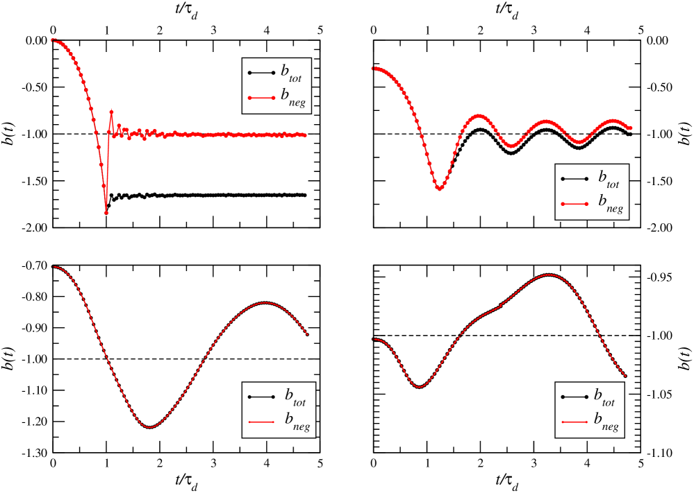
Figure 2: Behavior of the virial ratio for all system particles (black line) and only for particles with negative total energy (red line) as a function of time for different values of the initial virial ratio. Upper left panel: $b_{0}=0$, upper right panel: $b_{0}=-0.3$, bottom left panel: $b_{0}=-0.7$ and bottom right pane:l $b_{0}=-1$.

This picture is conformed by Fig.3 that shows the fraction of particles $f_{p}(t)$ with positive energy as a function of time: we find $f_{p}(t)>0$ for $t>\tau_{D}$ and $b_{0}>-1/2$. On the other hand, for $b_{0}<-1/2$ there is no ejection and $f_{p}(t)=0\;\;\forall t$.

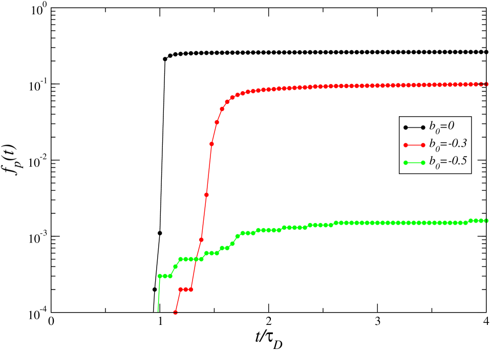
Figure 3: Fraction of the particles with positive energy function of time for different values of $b_{0}$: for $b_{0}<-1/2$ there is no ejection of particles.

As long as the spherical structure has uniform density the gravitational radius

$$R_{g}(t)=-\frac{3}{5}\frac{GM^{2}}{W(t)}\;,$$ (20)

coincides with the physical radius. From the analysis of the behavior of $R_{g}(t)$ shown in Fig.4 we may conclude that minimal size of the structure also depends on $b_{0}$. In particular, the minimal size $r_{min}\ll R_{0}$ is reached when $b_{0}\rightarrow 0$. while for $b_{0}<-1/2$ the size of the structure is almost unchanged.

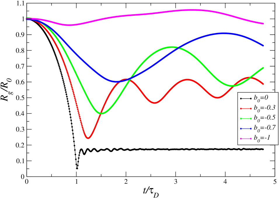
Figure 4: Gravitational radius of the structure as function of time for different initial virial ratio $b_{0}$.

In summary we have found that there is a clear difference between the behaviors of the relevant physical quantities for different initial virial ratio, particularly when the $b_{0}$ is smaller or larger than $b_{0}^{c}\approx-1/2$. In what follows we will study the statistical properties of the resulting quasi-equilibrium structure: we firstly, in Sect.4, discuss the problem of “mild relaxation”, i.e. $b_{0}<b_{0}^{c}$, to then pass in Sect.5 to the problem of “violent relaxation” for $b_{0}>b_{0}^{c}$. In Sect.7 we will consider the problem of understanding the origin the (approximate) value of $b_{0}^{c}$.

4 Mild relaxation and the Lynden-Bell predictions

Let us firstly discuss the case $b_{0}=-1$. Hereafter, we identify the center of the structure as the point in which the potential is minimum: alternative definitions (i.e. the center of mass) do not change qualitatively the results discussed below. The density profile is shown in Fig.5 (upper left panel) together with the cut-off Lynden-Bell distribution (see Sect.2.1), which nicely fits the measured behavior. A more detailed comparison of the results of N-body simulations with the predictions of the Lynden-Bell theory can be found in Worrakitpoonpon (2011), where it is discussed that also the energy and velocity distributions are in good agreement with the theoretical behaviors. The density profile can be best-fitted by a function of the type

$$n(r)=n_{c}\exp(-(r/r_{c})^{\eta})\;,$$ (21)

where $\eta\approx 2$. In addition we find that the characteristic length scale $r_{c}$ is of the same order $R_{0}$, implying that the system has not gone through a drastic change of shape and size. Rather it is only slightly changed so that particles have rearranged their positions and velocities to find a quasi-equilibrium configuration.

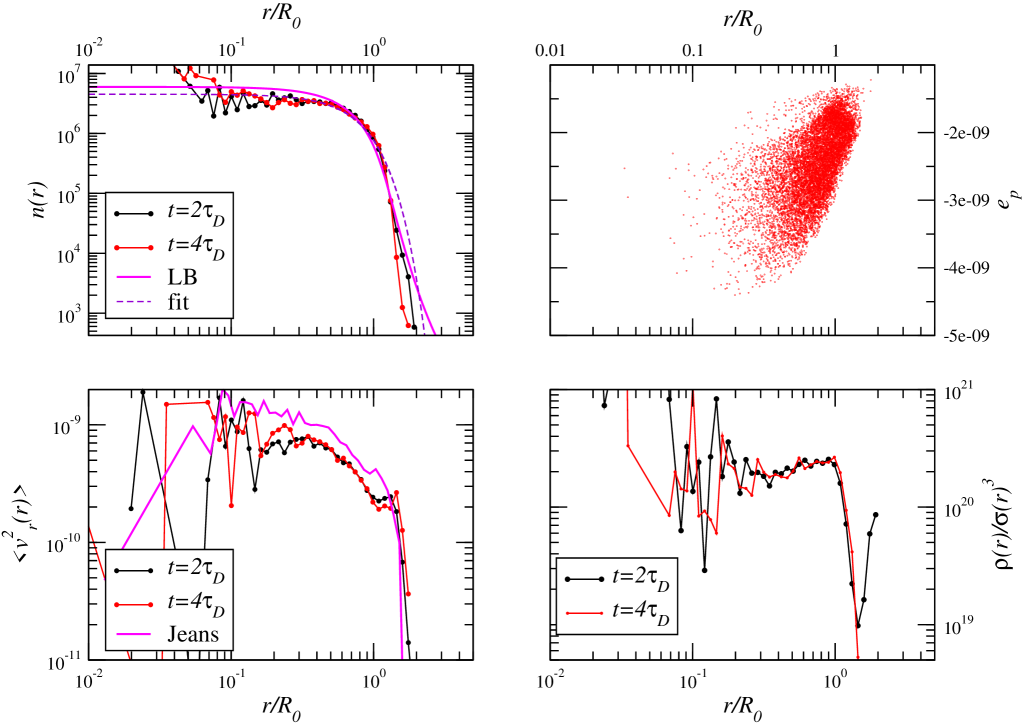
Figure 5: Behavior of some statistical quantities for the case $b_{0}=-1$. Upper left panel: density profile together with the prediction of the Lynden-Bell theory (LB) and the best fit with Eq.21. Upper right panel: energy per particle $e_{p}$ as a function of the distance from the center at $t=4\tau_{D}$. Bottom left panel: mean square value of the radial velocity together with the prediction of the Jeans equation (Eq.24). Bottom right panel: phase space density $\rho/\sigma^{3}(r)$.

In Fig.5 (upper right panel) it is also shown the behavior of the energy $e^{i}_{p}$ of the $i^{th}$ particle as a function of its distance from the center. We may note that $e^{i}_{p}<0\;\;\forall i$, which corresponds to the fact that all particles are bound: note no clear correlation between energy and spatial position is detected.

For an isotropic radial density profile, $\rho(r)$, one may solve, analytically or numerically, the Jeans equation to get the corresponding velocity dispersion, $\sigma^{2}(r)$ (Hernquist, 1990; Tremaine et al., 1994). The Jeans equation is

$$\frac{1}{\rho(r)}{{d(\overline{v_{r}(r)}^{2}\rho(r))}\over{dr}}+\alpha(r)\frac{\overline{v_{r}(r)}^{2}}{r}=-{{d\Phi}\over{dr}}\;.$$ (22)

In the previous equation $\sigma(r)=\overline{v_{r}(r)}^{2}$ is the velocity dispersion in the radial direction,

$$\alpha(r)=2-\frac{\overline{v_{t}(r)}^{2}}{\overline{v_{r}(r)}^{2}}\;,$$ (23)

is the the anisotropy parameter and $v_{t}(r)$ is the velocity in the transversal direction. When $\overline{v_{t}(r)}^{2}=\overline{v_{r}(r)}^{2}$ the velocity anisotropy terms are zero and Eq.22 can be rewritten as

$$\overline{v_{r}(r)}^{2}=\frac{1}{\rho(r)}\int_{r}^{\infty}\frac{\rho(y)GM(y)}{y^{2}}dy\;,$$ (24)

with the boundary condition

$$\lim_{r\rightarrow\infty}\overline{v_{r}(r)}^{2}\rho(r)=0\;.$$ (25)

It is interesting to note that the Jeans equation (Eq.24) is reasonably well satisfied in the time range we consider (Fig.5 — bottom left panel): this implies that the stationary state is well described by a stationary solution of the Vlasov equation, i.e. it is a collisionless stationary state. It should be noticed that although the velocity anisotropy (Eq.23) is different from zero (see below), the perturbation to the Jeans equation due to such a term does not sensibly affect the agreement between the measured $\overline{v_{r}(r)}^{2}$ and Eq.24. (We will come back on this point in Sect.5.) Finally we note that the phase-space density $\rho/\sigma^{3}(r)$, where $\sigma^{2}\equiv\langle v^{2}_{r}(r)\rangle$ is about flat, with a sharp decay for $r\rightarrow R_{0}$.

A statistical measure of the amount of energy that all particles have exchanged can be defined as follows

$$\langle\Delta^{2}(t)\rangle=\frac{1}{N(N-1)}\frac{\sum_{i,j=1\;i\neq j}^{N}(e_{p}^{i}(t)-e_{p}^{j}(t))^{2}}{\langle e(t)\rangle^{2}}$$ (26)

where $e_{p}^{i}(t)$ the average energy per particle is defined as

$$\langle e(t)\rangle=\frac{\sum_{i=1}^{N_{t}}e_{p}^{i}(t)}{N}\;.$$ (27)

One may see from Fig.6 that $\langle\Delta^{2}(t)\rangle$ oscillates in phase with the virial ratio (see Fig.2) and that the amount of energy exchanged by all particles is smaller than $10\%$ during the whole time range considered.

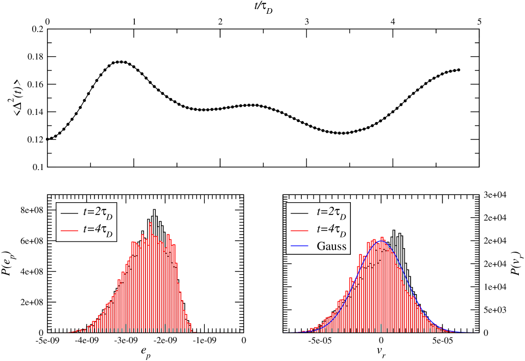
Figure 6: Other statistical quantities for the case $b_{0}=-1$. Upper panel: particle energy fluctuations (see Eq.26). Bottom left panel: energy distribution of all particles at different times. Bottom right panel: radial velocity distribution of particles at different times together with a the best fir with a Gaussian function.

The case $b_{0}=-0.7$ does not show substantial differences with respect to the $b_{0}=-1$ case (see Figs.7-8). The prediction of the Jeans equation for the velocity dispersion shows again that the system is well described by the collision-less limit (neglecting the term $\alpha(r)$ in Eq.22). The density profile is still characterized by a constant behavior at small scales followed by a sharp decay of the type described by Eq.21, although $r_{c}$ is smaller than for the $b_{0}=-1$ case, implying a larger contraction during the collapse phase. Correspondingly, particle energies, for $t>2\tau_{D}$, are larger than for the $b_{0}=-1$ case, but still $e_{p}^{i}<0\;\forall i$. The exchange of energy among particles (Eq.26) was more efficient during the first oscillation of the system, i.e. for $0<t<1.5\tau_{D}$, and it is then reduced at later times, in agreement with the fact that the system is relaxed into a QSS: each particle move in a time independent potential and the energy of each particle is conserved modulo two-body collisions.

Figure 7: As Fig.5 but for the case $b_{0}=-0.7$.

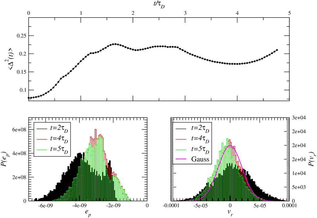
Figure 8: As Fig.6 but for the case $b_{0}=-0.7$.

5 Violent Relaxation and the formation of the power-law tail of the density profile

We now present the main results of N-body simulations for the case in which the initial virial ratio is $-1/2<b_{0}\leq 0$. In this case during the collapse the size of the system undergoes to a large compression and a fraction of the particles gain a certain amount of kinetic energy so that they will have velocities larger than the escape one.

In Fig.9 (upper left panel) it is shown the density profile at $t>\tau_{D}$: one may note that an almost asymptotic behavior is reached already at $t\mathrel{\hbox to0.0pt{\lower 3.0pt\hbox{$\mathchar 536\relax$}\hss}\raise 2.0pt\hbox{$\mathchar 318\relax$}}\tau_{D}$. However, at later times the profile is almost identical but for the fact that the tail extends to larger scales. We find that the density profile is well approximated by Eq.10 where $r_{c}\approx 0.03R_{0}$ and $\zeta=4$. Note that the density profile has two different regimes: at small scales, i.e. $r<r_{c}$, the structure corresponds to an homogeneous sphere with constant density $n(r)\approx n_{c}$ while at large scales, i.e. $r>r_{c}$ it shows a $r^{-4}$ decay. As already mentioned we find that $r_{c}\approx\ell=0.55R_{0}(4\pi/N)^{1/3}$. The minimal radius $r_{min}$ reached by the structure during the collapse can be defined as the radius, measured from the center of mass, enclosing the $90\%$ of the mass. It is found that $r_{min}\approx r_{c}\approx\ell$.

In the upper right panel of Fig.9 it is shown the diagram radial distance-total energy only for the bound particles. One may note that for $r>r_{c}$ the points follows an approximate $e_{p}\sim r^{-1}$ behavior. This can be easily explained by considering that particles at distances $r>r_{c}$ move in a constant gravitational potential generated by particles with $r<r_{c}$. In this situation particle velocities should display a Keplerian behavior $v_{r}\sim r^{-1/2}$ so that that $e_{p}\sim v_{r}^{2}\sim r^{-1}$. This behavior is confirmed by considering (bottom right panel of Fig.9) the behavior of the average radial component of the velocity as a function of the radial distance. (The average has been performed in radial shells). Indeed, we find that

$$\langle v_{r}^{2}(r)\rangle\equiv\sigma^{2}(r)=\frac{\sigma_{c}^{2}}{1+\left(\frac{r}{r_{c}}\right)}\;,$$ (28)

where $\sigma_{c}^{2}$ is a constant and $r_{c}$ has been determined from the density fit (Eq.10). The behavior of Eq.28 is similar to the one of the density in Eq.10: it is constant at small scales and it decays for $r>r_{c}$. As time passes, a few particles reach a larger and larger distances from the center of the structure, leaving however unchanged the functional behavior of Eq.28.

Given the behaviors of Eq.10 and Eq.28 we may fit the phase-space density with (see the bottom left panel of Fig.9)

$$\frac{\rho(r)}{\sigma^{3}(r)}=\frac{n_{c}}{1+\left(\frac{r}{r_{c}}\right)^{4}}\times\sqrt{\frac{1+\left(\frac{r}{r_{c}}\right)}{\sigma_{c}^{2}}}^{3}\;.$$ (29)

Thus we find that the phase-space density is $\rho/\sigma^{3}\propto r^{-5/2}$ for $r>r_{c}$ while it is almost flat at smaller scales.

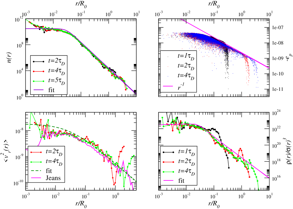
Figure 9: As Fig.5 but for $b_{0}=0$. The best fit of the density profile with Eq.10 is also shown, together with the fit given by Eq.28 of mean square value of the radial velocity and the fit given by Eq.29 for the phase space density.

It is interesting to note, as firstly shown in the pioneering paper by van Albada (1982) and then studied in detail by Trenti, Bertin & van Albada (2005), that the QSS formed after the collapse is dominated, in the outer regions where the density scales as $n(r)\sim r^{-4}$, by radial orbits. This is shown by the behavior of $\alpha(r)$ (Eq.23) as a function of the radial distance (see Fig.10). On the other hand for the QSS obtained starting from $b_{0}=-1$ the velocity dispersion is by dominated by its transversal component.

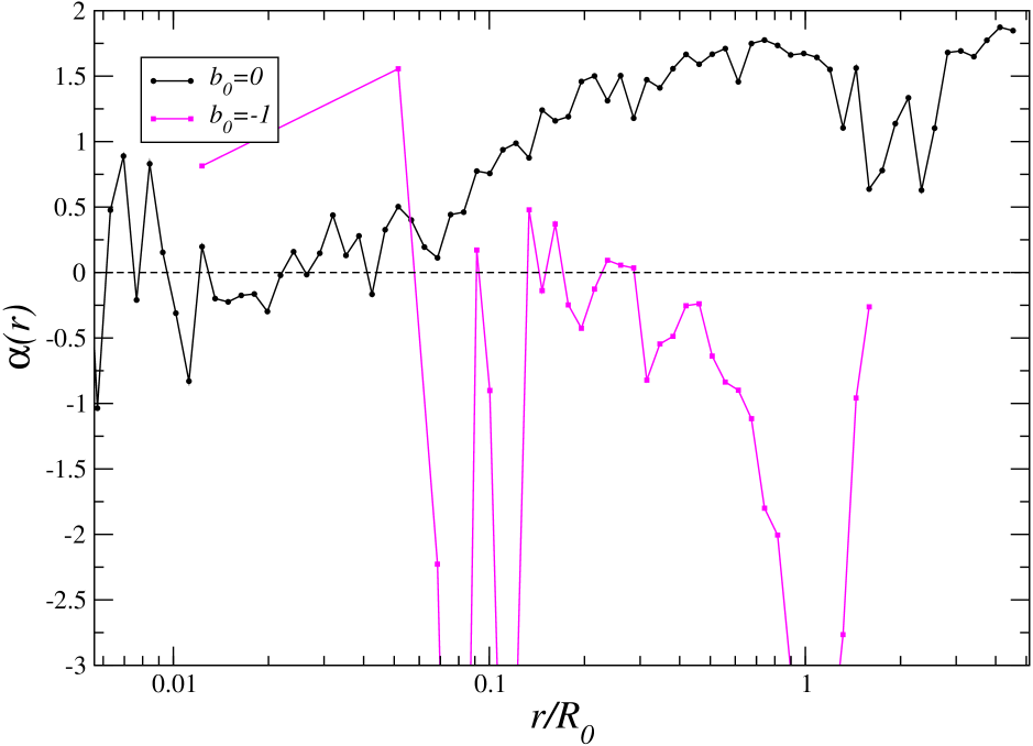
Figure 10: Velocity anisotropy for the case $b_{0}=0$ and $b_{0}=-1$. When $\alpha(r)>0$ the velocity dispersion for $b_{0}=0$ is by dominated by its radial component while for $b_{0}=-1$ by its transversal one.

The behavior of $\Delta^{2}(t)$ (Eq.26) (see the upper panel of Fig.11) shows that in this case particles exchange a substantial amount of energy in the time range $0.7\tau_{D}<t<1.2\tau_{D}$, while before and after the central collapse phase the energy per particle is very well conserved. Differently from the $b_{0}<-1/2$ case, during the collapse a fraction of the particles change their total energy by a relevant factor so that some of the particles may gain enough kinetic energy to escape from the system. The $b_{0}>-1/2$ case corresponds to an almost instantaneous collapse followed by a rapid relaxation toward a QSS. The particle energy distribution (Fig.11 bottom left panel) shows that some of the particles have indeed positive energy. Finally the radial velocity distribution (Fig.11 bottom right panel) is reasonably well fitted by a Gaussian function.

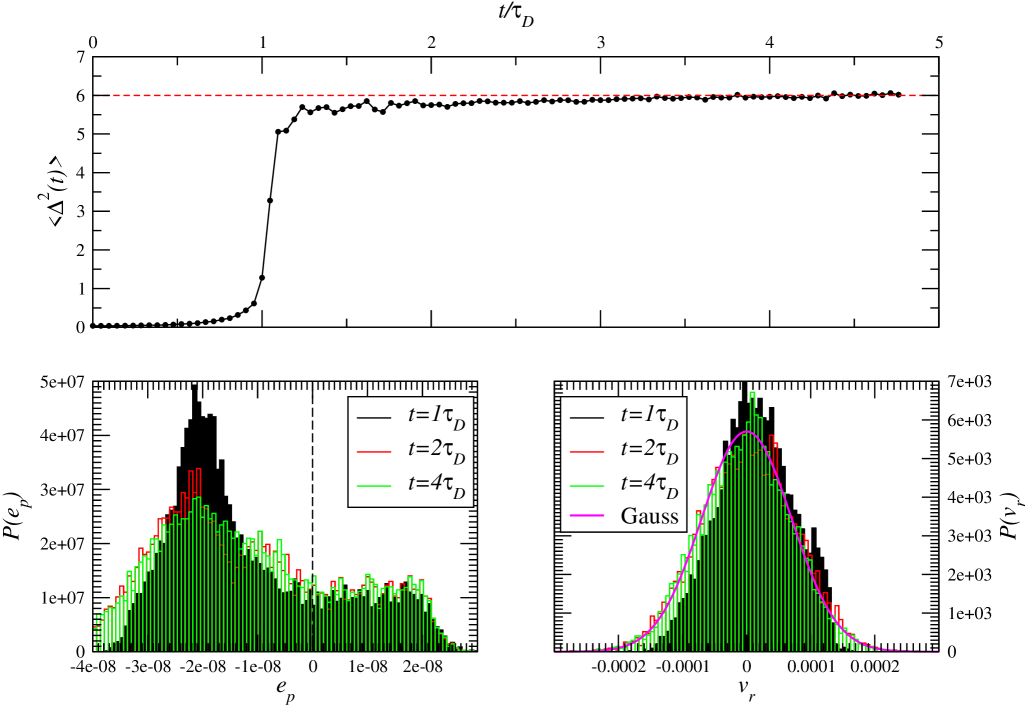
Figure 11: As Fig.6 but for $b_{0}=0$.

Behaviors similar to the ones shown in Figs.9-11 are found for the case in which the initial virial ratio is $b_{0}=-0.3$ (see Figs.12-13). However, due a the non zero initial velocity dispersion, the collapse is less peaked in time. The density profile is again well approximated by Eq.10, but in this case $r_{c}=0.2R_{0}$ i.e. it is about ten times larger than for the $b_{0}=0$ case. Correspondingly we find $n_{c}(b_{0}=-0.3)<n_{c}(b_{0}=0)$, i.e. the structure of the QSS is much less compact. Also the behaviors of $\langle v_{r}^{2}(r)\rangle$ and of $\rho(r)/\sigma^{3}(r)$ are well described by Eqs.28-29 although with different parameters. Finally $\Delta^{2}(t)$ shows that there is a smaller exchange of energy during the collapse phase than in the $b_{0}=0$ case, but still much larger than for $b_{0}<-1/2$. In brief, in this case the collapse is less violent and the fraction of particles with positive energy for $t>\tau_{D}$ is greatly reduced with respect to the $b_{0}=0$ case (see Fig.4).

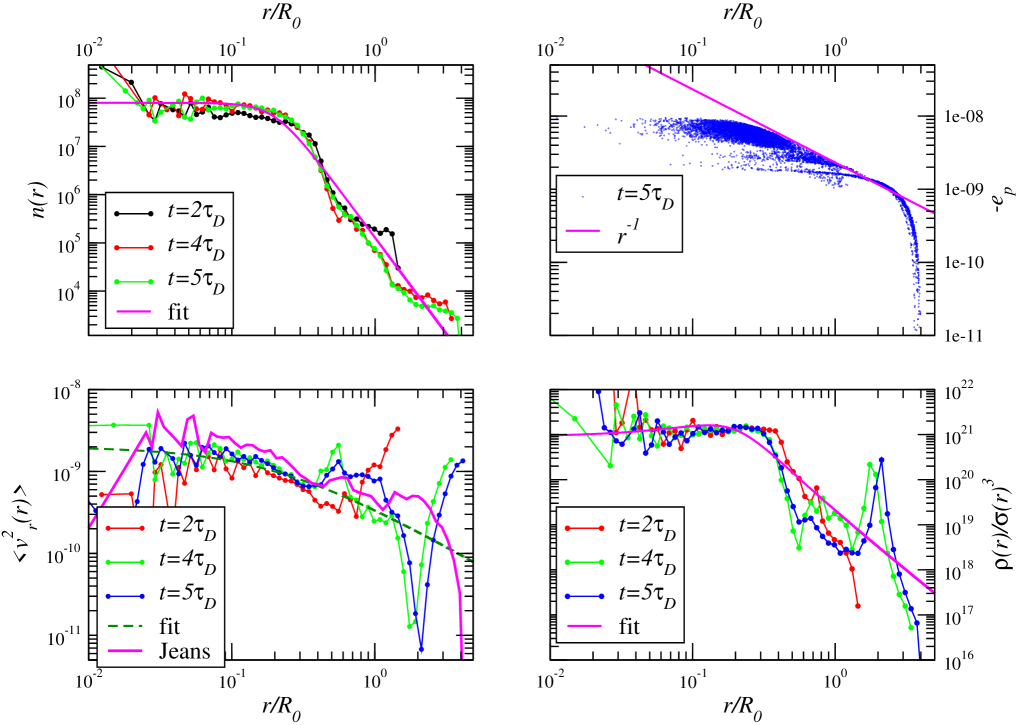
Figure 12: As Fig.12 but for the case $b_{0}=-0.3$.

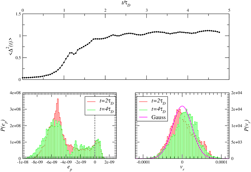
Figure 13: As Fig.11 but for the case $b_{0}=-0.3$.

6 The origin of the power law tail in the violent relaxation case

We now introduce a simple physical model with the aim of describing the dynamics of bound particles with $r>r_{c}$ when $b_{0}>b_{0}^{c}\approx-1/2$. We then show that this model allows us to capture the essential ingredients that originate the power law $r^{-4}$ tail in the density profile (Eq.10).

6.1 A simple physical model

We suppose that the bound particles with $r>r_{c}$ for $t>\tau_{D}$, are only subjected to the gravitational field of the core with mass

$$M_{c}=4\pi\int_{0}^{r_{c}}\frac{n_{c}m}{1+(r/r_{c})^{4}}r^{2}dr\approx\frac{4\pi}{3}n_{c}r_{c}^{3}m\;,$$ (30)

so that the equation of motion for one of these particles is simply

$$\frac{d^{2}r}{dt^{2}}=-\frac{GM_{c}}{r^{2}}\;.$$ (31)

We can integrate Eq.31 to get

$$\frac{1}{2}\left(\frac{dr}{dt}\right)^{2}=\frac{GM_{c}}{r}-\epsilon_{0}$$ (32)

where we defined

$$\epsilon_{0}=\frac{GM_{c}}{r_{0}}-\frac{1}{2}v_{0}^{2}\;,$$ (33)

and $r_{0},v_{0}$ are respectively the initial position and velocity at the initial time $t_{0}$.

The initial conditions at $t_{0}$ are specified as follows. We take the origin of the time at $t_{0}=\tau_{D}$, i.e. the time of maximum collapse of the system. In this situation particles are confined in a spherical volume of radius $r_{min}\approx r_{c}$, the minimal radius of the system during the collapse. As particles forming the density power-law tail must be bound, their energy is negative, i.e. $\epsilon_{0}=-e_{p}(\tau_{D})>0$ at $t=\tau_{D}$. We make the hypothesis that this energy is conserved at later times. This hypothesis is both confirmed by the simulation (see below) and compatible with the fact that the system is a quasi-stationary equilibrium for $t>\tau_{D}$. Indeed, in a QSS — defined in the mean field limit — each particle moves in a time independent potential, and therefore has exactly fixed energy. In principle, any change of energy is due to finite $N$ effects, which are, however, relevant only on a much long time scale than the one considered here. Particles velocities are assumed to be oriented outwards, an hypothesis that agrees with the fact that after the collapse the velocity dispersion is by dominated by its radial component (see Fig.10).

Bound particles may have a maximum velocity such that $e_{p}^{M}=0$, i.e. for

$$v_{0}^{M}=\sqrt{\frac{2GM_{c}}{r_{0}}}\;,$$ (34)

so that also the velocity is bounded in $0<v_{0}\leq v_{0}^{M}$. By defining

$$r_{H}=\frac{GM_{c}}{2\epsilon_{0}}$$ (35)

we can rewrite Eq.32 as

$$\frac{dr}{\sqrt{2r_{H}r-r^{2}}}=\sqrt{2\epsilon_{0}}\frac{dt}{r}\equiv d\eta\;,$$ (36)

where the last equality defines the variable $\eta$. Eq.36 has solution in a parametric form

$$r(\beta)=r_{H}(1+\sin(\beta))$$ (37)

$$t(\beta)=\frac{r_{H}}{\sqrt{2\epsilon_{0}}}\left(\beta-\cos(\beta)-\beta_{0}+\cos(\beta_{0})\right)$$ (38)

where

$$\beta_{0}=\sin^{-1}\left(\frac{2r_{0}}{r_{H}}-1\right)\;.$$ (39)

Thus for $\beta=\beta_{0}$ we have $t=0$ and $r(0)=r_{0}$. Therefore we obtain

$$r(\beta)\leq r=\frac{2GM_{c}}{(v_{0}^{M})^{2}-(v_{0})^{2}}\;\;\forall\beta\;,$$ (40)

where the equality holds for the peaks of the sinusoidal function. By inverting Eq.40 and using Eq.34 we find

$$v_{0}\approx\sqrt{(v_{0}^{M})^{2}-\frac{2GM_{c}}{r}}=v_{0}^{M}\sqrt{1-\frac{r_{0}}{r}}\;.$$ (41)

The behavior of the radial distance $r$ as a function of the initial velocity $0<v_{0}\leq v_{0}^{M}$, computed from Eqs.37-38, is plotted in Fig.14 for $t=3/2\tau_{D}$. Similarly in Fig.15 it is plotted $r(t)$ for different values of the initial velocity. One may note that only the high velocity particles, for which $v_{0}\approx v_{0}^{M}$, may reach a distance of the order of the initial system’s radius $R_{0}$. As time passes, the particles with the highest velocity increases their radial distance to $r>R_{0}$. At a time of the order of $\approx 3/2\tau_{D}$ the structure has already reached its (almost) asymptotic shape for $r_{c}<r\mathrel{\hbox to0.0pt{\lower 3.0pt\hbox{$\mathchar 536\relax$}\hss}\raise 2.0pt\hbox{$\mathchar 316\relax$}}R_{0}$: while at larger scales and at later times, a few particles may arrive to larger and larger distances.

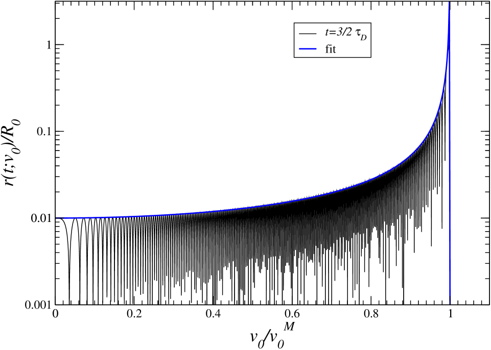
Figure 14: Behavior of the distance $r(t;v_{0})$ reached by a particle after a time $1/2\tau_{D}$ from the collapse, as a function of its initial velocity $v_{0}\in[0,v_{0}^{M}]$ (from Eqs.37-38). The behavior of Eq.40 is also plotted.

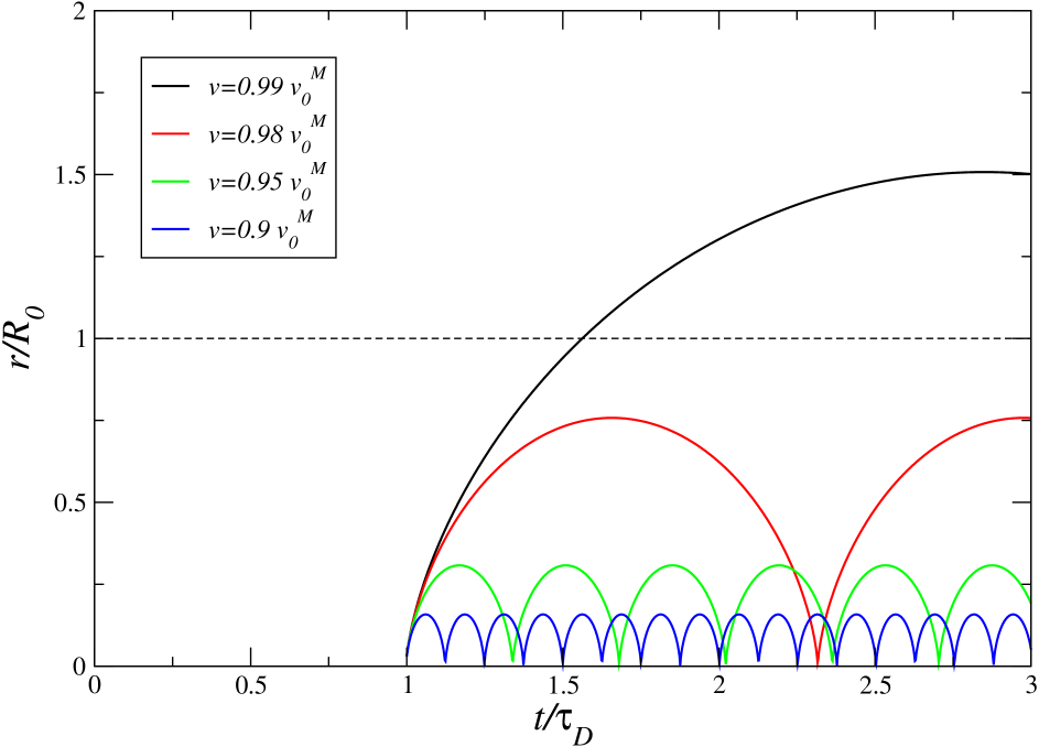
Figure 15: Behavior of the distance $r(t)$ as a function of time for different values of its initial velocity $v_{0}$ (from Eqs.37-38).

6.2 Shape of the density profile

Let us now compute, under some simple approximations, the density profile resulting from this simple physical model. We suppose that all particles have, at the same initial time $\tau_{D}$, the same initial position $r_{0}\leq r_{c}$. In this approximation, given a certain distribution of initial velocities $p(v_{0})$, we find that the radial density profile, for $t\mathrel{\hbox to0.0pt{\lower 3.0pt\hbox{$\mathchar 536\relax$}\hss}\raise 2.0pt\hbox{$\mathchar 318\relax$}}2\tau_{D}$ (see Fig.15), is given by

$$n(r)\approx\frac{1}{4\pi r^{2}}Np(v_{0})\frac{dv_{0}}{dr}=\frac{GM_{c}Np(v_{0})}{4\pi r^{4}\sqrt{(v_{0}^{M})^{2}-\frac{2GM_{c}}{r}}}\;.$$ (42)

One may note that from Eq.41 we find that $v_{0}\approx v_{0}^{M}$ for $r>r_{c}$, so that in this limit Eq.42 becomes

$$n(r)\approx\frac{GM_{c}N}{4\pi r^{4}v_{0}^{M}}p(v_{0}^{M})\;,$$ (43)

thus showing the $r^{-4}$ decay in the best fit of measured $n(r)$ (Eq.10).

Although in the derivation of Eq.42 we made important simplifications, we now show that the hypotheses used allow us to capture the main elements of the problem. We may relax these assumptions by allowing that the initial particle positions $r_{0}$ also have a certain PDF $f(r_{0})$. In this case we need to integrate Eqs.37-38 numerically as follows:

• We extract the initial conditions $[r_{0},v_{0}]$, such that $0<r\leq r_{c}$ and $0<v_{0}\leq v_{0}^{M}$, from the assigned initial position and velocity PDFs $f(r_{0})$ and $p(v_{0})$.

• We fix the time $t>\tau_{D}$ at which we compute the profile.

• We then find from Eq.38 the value $\beta=\beta(t,r_{0},v_{0})$ and then from Eq.37 $r(t)=r(t,r_{0},v_{0})$.

• We repeat the iteration $N$ times and we can thus construct numerically, from the resulting distribution of distances $r(t)$, the density profile at time $t$.

As an example (see Fig.16) we have assumed a Gaussian velocity distribution $p(v_{0})$ with zero mean and variance $(v_{0}^{M})^{2}/\alpha$, where $\alpha>1$ is a free parameter, and we have considered only particles with $v_{0}>0$. In addition we have taken a uniform distance $r_{0}$ distribution such that $f(r_{0})\neq 0$ only for $r_{0}\in[0,r_{c}]$. We have tested that no sensible differences are detected as long as $\alpha$ is not large enough to get a too small value of $p(v_{0}^{M})$: in particular, when $Np(v_{0}^{M})<1$ a particle cannot neither be ejected nor form the $r^{-4}$ tail. In principle, one should also consider the correlations between $r_{0}$ and $v_{0}$ and the fact that particles have a distribution of initial times: however these complications do not significantly alter the result of Eq.43.

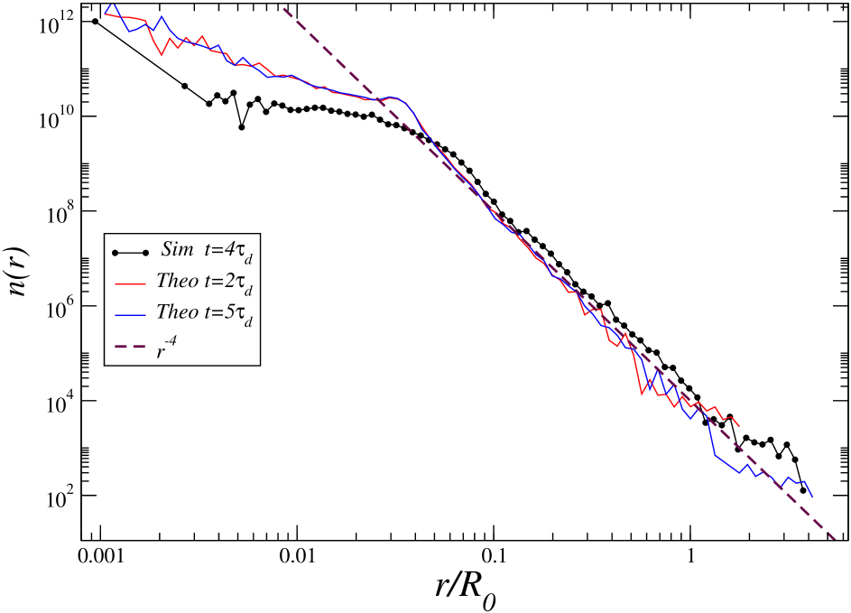
Figure 16: Behavior of the theoretical radial density $n(r)$ computed with the Monte-Carlo method described in the text at different times. The normalization is arbitrary.

Finally we note that as time passes, for $t>\tau_{D}$, the power-law tail extends to larger and larger scales (see Fig.9). This is simply explained by the behaviors shown in Figs.14-15: the largest distance reached by the particles with highest velocity also increases with time, although the precise manner in which this occurs depends in a very detailed way on the value on the properties of $p(v_{0})$ for $v_{0}\rightarrow v_{0}^{M}$.

7 The critical value of the initial virial ratio

We now consider the question of what determines the critical value of the initial virial ratio for having or not ejection (and thus the formation of the $n(r)\sim r^{-4}$ power law tail) to be $b_{0}^{c}\approx-1/2$. We would like to stress that the precise value $b_{0}^{c}$ must be a function of $N$, as collisional and discrete effects, although represent perturbations, are also present in the collapse phase (Joyce et al., 2009).

As mentioned in Sect.2.2, the mechanism of energy and mass ejection is based on the fact that a fraction of the particles, and particularly those that lie at the boundary of the system at the initial time, lag behind with respect to the others during the collapse, i.e. at $t<\tau_{D}$. Particles in the bulk collapse approximately satisfying the condition of homologous contraction (Eq.6). The question is whether this is also satisfied when $b_{0}<0$.

In Fig.17 we plot, for different values of the initial virial ratio $b_{0}$, particle positions at time $t$ (for $t=1/4\tau_{D},3/4\tau_{D}$) as a function of their positions at time $t=0$. We have considered an average in shells where these are taken at $t=0$; we then plot the average value in each shell together with the r.m.s. error. One may see that for $b_{0}=0$ the two curves do not overlap, while this marginally occurs for $b_{0}=-0.3$. In this case the homologous contraction is a reasonable approximation of the collapse.

For smaller values of the initial virial ratio, i.e. $b_{0}=-0.7,-1$, there is a substantial overlapping of the curves at different times, which means that particles originally belonging to different shells interchange their positions. This implies that the collapse cannot be anymore approximated as homologous because different shells largely overlap well before $\tau_{D}$.

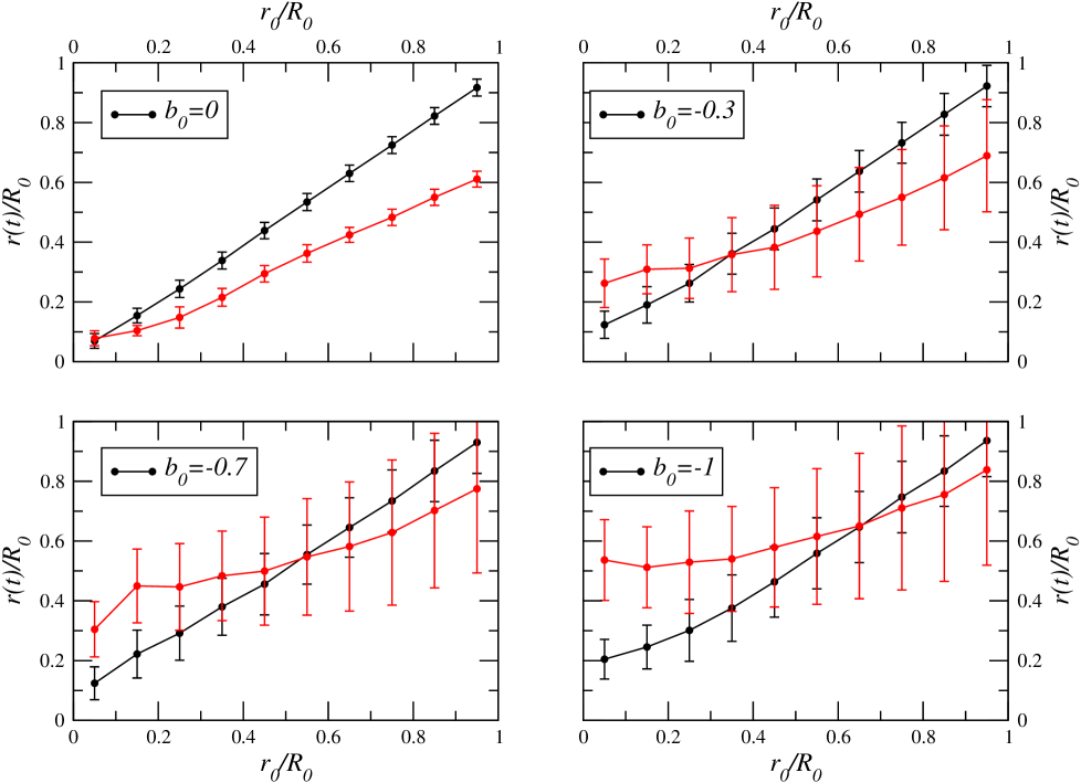
Figure 17: Behavior of the position at time $t$ (black dots $t=1/4\tau_{D}$, red dots $t=3/4\tau_{D}$) as a function of the initial position $r_{0}$, averaged in shells, for different values of the initial virial ratio (see caption).

The key mechanism of the growth of the time lag is thus eliminated when particles have initially high enough velocity dispersion, as different shells cross each other well before $\tau_{D}$. Thus particles from the outer shell arrive at different time at the center and they do not gain the necessary energy to escape from the system.

Finally it should be noted that the analysis presented in this section holds only for water bag initial conditions, and that a different initial spatial and velocity distribution can lead to very different behaviors. For instance, Trenti, Bertin & van Albada (2005) have found that initial conditions with equal virial ratio but different spatial distributions, as for example by generating clumpy distributions, lead to significantly less mass ejection. A similar result was found by Trenti & Bertin (2006) when particles were initially distributed in a shell rather than in a sphere. Given that the precise amount of mass and energy ejection is determined by the coupling of the growth of perturbation with the finite size of the system it is difficult to develop a general argument which is valid for different initial conditions and a more detailed consideration of each case is needed.

8 Discussion and conclusion

The collapse of an isolated, uniform and spherical cloud of massive particles interacting by Newtonian gravity represents a paradigmatic example for the formation of quasi equilibrium states. It is indeed well known, since the earliest N-body simulations that, when initial velocities are set to zero, this system collapses in a relatively short time scale $\tau_{D}\approx\sqrt{G\rho_{0}}^{-1}$ reaching a configuration which satisfies the virial theorem $b(t)=2K/W\approx-1$. The collective relaxation process acting on such a short time scale and the statistical properties of the formed quasi equilibrium state have been considered in this paper both by performing numerical simulations and by an attempt to elaborate a physical model able to capture the essential elements of the problem.

In particular, the initial conditions of simulations are generated by randomly placing $N$ particles with average mass density $\rho_{0}$ in a spherical volume and characterized by different initial virial ratio $0\geq b_{0}\geq-1$. Thus, only two parameters, i.e., $N,b_{0}$, define the initial conditions: in this paper we have varied $b_{0}$ in the range $[-1,0]$ while in Joyce et al. (2009) we have considered, for the case $b_{0}=0$, simulations with different number of points $N$.

The system thus collapses under its self-gravity and then it forms a virialized structure. This does not represent an equilibrium state in the thermodynamics sense. Indeed, two body collisions, which have a time scale of about $\tau_{2}\approx\tau_{D}\ln(N)/N$ will cause a slow evaporation of particles from it (Binney & Tremaine, 1994). For this reason the state formed after $\tau_{D}$ is called a quasi stationary state (QSS) (Dauxois et al., 2003; Campa et al., 2008) .

By considering N-body simulations with different initial virial ratios, we have identified a critical initial virial ratio $b_{0}^{c}\approx-1/2$ separating the formation of two qualitatively different kind of QSS. When $-1\leq b_{0}<-1/2$ the collapse consists in a series of damped oscillations, the first of which one has larger amplitude. The system thus approximately maintains its original size. The density profile characterizing the virialized QSS is well fitted by the predictions of the Lynden-Bell distribution with a cut-off by considering the system confined in a box (Levin et al., 2008). This is characterized by an abrupt decay of the density at a scale $r_{c}\approx R_{0}$. The Lynden-Bell predictions strictly holds for a confined system: however it was found that the theory does not depend sensibly on the cut-off value. This approach is thus useful to understand the properties of gentle kind of collective relaxation which occurs when the systems is initially in a configuration which is close enough to the virial equilibrium.

On the other hand, for $-1/2\leq b_{0}\leq 0$ the system size undergoes to a large compression and a part of its mass and energy is ejected. Finite $N$ fluctuations in the initial spatial particle configuration generate density perturbations which grow during the collapse. When $b_{0}=0$ such a dynamical problem can be treated, when boundaries effects are neglected (i.e. in the limit $R_{0}\rightarrow\infty$) as the growth of perturbations in a contracting universe. When fluctuations at a scale $r_{min}$ of order of the size of the system go non-linear the collapse is stopped (Aarseth et al., 1988; Boily & Athanassoula, 2006; Boily et al., 2002; Joyce et al., 2009).

During such the collapse some particles gain enough kinetic energy that can be ejected from the system. The ejection mechanism was studied in detail by Joyce et al. (2009) where it was shown to be related to a boundary effect. Particles initially placed close to the boundaries arrive later than the others toward the center, moving, for a short time interval, in a rapidly varying potential field generated by the particles which have already inverted their motion from inwards to outwards. In this way they gain some kinetic energy, so that some particles have positive energy $e_{p}>0$. The density profile $n(r)$ of the bound system formed after the collapse is characterized by a core, where $\rho(r)\sim const.$ and by an halo in which $n(r)\sim r^{-4}$. The former behavior can be understood by considering that the distribution function of the core is given by that of a fully degenerate Fermi gas: this can be obtained again from the cut-off Lynden-Bell distribution, by letting the cut-off to extend to infinity so that particles can move far away from the center. In this case it forms a core-halo structures, with a dense core a diluted halo (Levin et al., 2008). The Lynden-Bell theory cannot however be used to derive the properties of the halo, i.e. that the radial density decays as $n(r)\sim r^{-4}$.

In order to understand the formation of such a power-law tail we have introduced a simple physical model based on a few ingredients, namely that that: (i) at the time of maximum contraction, i.e. $t\approx\tau_{D}$, particles are confined in a small phase-space region, (ii) particles energy may be close to, or larger than, the escape one and (iii) particles forming the power-law tail move in a central and constant gravitational potential generated by the mass of the core $M_{c}$ at $r<r_{c}$. With these assumptions a density profile with a power-law tail is naturally formed. We conclude that the behavior $n(r)\sim r^{-4}$ is the typical density profile that is obtained when the initial conditions are cold enough that ejection of mass and energy occurs.

The critical virial ratio $b_{0}^{c}$ separating the two situations in which the power-law profile is formed, and mass ejection occurs, can be understood by considering that when the initial velocity dispersion is large enough the contraction is no more homologous. Therefore different shells may overlap before the final collapse phase at $t\approx\tau_{D}$ and the mechanism underlying the gain of energy for the outer particles cannot be working anymore.

Finally it is interesting to note that cold dark matter halos in cosmological simulations (Navarro et al., 1996; Moore et al., 1988, 2001; Navarro et al., 1997; Hansen, 2004; Navarro et al., 2004; Merritt et al., 2006) display a density profile such that $n(r)\sim r^{-1}$ at small scales and $n(r)\sim r^{-3}$ at large scales: these behaviors are not observed to form from the simple initial conditions we have chosen Also the phase space density has a different shape, decaying as $\rho/\sigma^{3}\sim r^{-1.875}$ at all scales in cosmological simulations (Navarro et al., 2004) while it displays a $r^{-5/2}$ behavior only at large enough scales, i.e. $r>r_{c}$, in the case of structures formed from the initial conditions we considered (when $b_{0}^{c}>-1/2$). This difference maybe originated by that the fact that cosmological halos are formed from more complicated initial conditions than the case we considered. However, one should also consider that cosmological halos are formed in a complex backgrounds so that the hypothesis that they are isolated structures maybe not be a valid assumption. In addition, there is a continuous mass accretion so that neither the total mass nor the total energy are conserved. A more focused study of these features will be presented in a forthcoming work.

I acknowledge Roberto Capuzzo-Dolcetta, Massimo Cencini, Umberto Esposito, Andrea Gabrielli, Michael Joyce, Yan Levin and Tirawut Worrakitpoonpon for useful discussions and comments.

References

- Aarseth et al. (1988) Aarseth S., Lin D., Papaloizou J., 1988, Astrophys. J., 324, 288
- Aarseth (2003) Aarseth S. J., 2003,Gravitational N-Body Simulations: Tools and Algorithms, Cambridge University Press
- Aarseth (1974) Aarseth S., 1974, Astron. Astrophys., 35, 237
- Arad & Johansson (2005) Arad I., Johansson P., 2005, Mon. Not. R. Astron. Soc., 362, 252
- Arad & Lynden-Bell (2005) Arad I., Lynden-Bell D., 2005, Mon. Not. R. Astron. Soc., 361, 385
- Bertin & Trenti (2003) Bertin G. & Trenti M., 2003, Astrophys.J., 584, 729
- Bertschinger (1985) Bertschinger E, 1985, Astrophys.J.Suppl., 58, 39
- Binney & Tremaine (1994) Binney J., Tremaine S., 1994, Galactic Dynamics, Princeton University Press
- Binney & Merrifield (1998) Binney J., Merrifield M.., 1998, Galactic Astronomy, Princeton University Press
- Boily & Athanassoula (2006) Boily C., Athanassoula E., 2006, Mon. Not. R. Astr. Soc., 369, 608
- Boily et al. (2002) Boily C., Athanassoula E., Kroupa P., 2002, Mon. Not. R. Astr. Soc., 332, 971
- Campa et al. (2008) Campa A., Giansanti A., Morigi G., Sylos Labini F., (Eds.), 2008, Dynamics and thermodynamics of of systems with long-range interaction: theory and experiments, AIP Conf. Proc., 970
- Cooray & Sheth (2002) Cooray A., Sheth R., 2002, Phys. Rep., 379, 1
- David &Theuns (1989) David M., Theuns T., 1989, Mon. Not. R. Astr. Soc., 240, 957
- Dauxois et al. (2003) Dauxois T., Ruffo S., Arimondo E., Wilkens M. (Eds). 2003 Dynamics and Thermodynamics of Systems with Long-Range Interactions, Lecture Notes in Physics, 602, Springer
- Dekel etal. (2003) Dekel A., Arad I., Devor J., Birnboim Y., 2003, Astrophys.J., 588, 680
- de Vaucouleurs (1948) de Vaucouleurs G., 1948 Ann.Astrophys., 11, 247
- Diemand etal. (2004) Diemand J., Moore B., Stadel J., 2004, Mon.Not.Roy.Astron.Soc., 353, 624
- Gabrielli et al. (2010) Gabrielli A., Joyce M., Marcos B., 2010, Phys.Rev.Lett.,105, 210602
- Graham et al. (2006) Graham A., et al. 2006, Astron.J., 132, 2701
- Heggies (2003) Heggies D., Hut P., 2003, The Gravitational Million-Body Problem Cambridge University Press
- Hansen (2004) Hansen S., 2004, Mon.Not.Roy.Astron.Soc., 352, L41
- Hénon (1964) Hénon M., 1964, Ann. Astrophys., 27, 1
- Hernquist (1990) Hernquist, L. 1990, Astrophys.J. 356, 359
- Hiotelis (2002) Hiotelis N., 2002, Astron. & Astrophys., 382, 84
- Joyce et al. (2009) Joyce M., Marcos B., Sylos Labini F., 2009, Mon. Not. R. Astr. Soc., 397, 775
- Joyce & Worrakitpoonpon (2012) Joyce M., Worrakitpoonpon T., 2012, Phys.Rev. E in the press arXiv:1012.5042v2
- Levin et al. (2008) Levin Y., Pakter R., Rizzato F., 2008, Phys. Rev., E78, 021130
- Chavanis & Sommeria (2008) Chavanis P.H & Sommeria J. 1998, Mon.Not.R.Astr.Soc., 296, 569
- Lynden-Bell (1967) Lynden-Bell D., 1967, Mon. Not. R. Astr. Soc., 167, 101
- Manrique etal. (2002) Manrique A., Raig A., Salvador-Solé E., Sanchis T., Solanes J. M., 2003, Astrophys.J., 593, 26
- Merritt et al. (2006) Merritt D., et al., 2006, Astron.J., 132, 2685
- Moore et al. (1988) Moore B., et al., 1988, Astrophys.J., 499, 5
- Moore et al. (2001) Moore B., et al., 2001, Phys.Rev, D64, 063508
- Navarro et al. (1996) Navarro J. F., Frenk C. S., White S. D. M., 1996, Astrophys. J., 462, 563
- Navarro et al. (1997) Navarro J. F., Frenk C. S., White S. D. M., 1997, Astrophys. J., 490, 493
- Navarro et al. (2004) Navarro J. F., et al., 2004, Mon.Not.Roy.Astron.Soc., 349, 1039
- Padmanabhan (1990) Padmanabhan T., 1990, Phys. Rept., 188, 285
- Peebles (1980) Peebles P. J. E., 1980, The Large-Scale Structure of the Universe. Princeton University Press
- Reed etal. (2005) Reed D et al., 2005, Mon.Not.Roy.Astron.Soc., 357, 82
- Roy & Perez (2004) Roy F., Perez J., 2004, Mon. Not. R. Astr. Soc., 348, 62
- Saslaw (2000) Saslaw W.C., 2000, The distribution of the galaxies, Cambridge University Press
- Syer & White (1998) Syer D., White S. D. M., 1998, Mon. Not. R. Astr. Soc, 293, 337
- Springel (2005) Springel V., 2005, Mon. Not. R. Ast. Soc., 364, 1105
- Springel et al. (2001) Springel V., Yoshida N., White S. D. M., 2001, New Astronomy, 6, 79
- Subramanian et al. (2000) Subramanian K., Cen R., Ostriker J. P., 2000, Astrophys.J., 538, 528
- Stiavelli & Bertin (1984) Stiavelli M. & Bertin G., 1984, Astron.Astrophys. 137, 26
- Stiavelli & Bertin (1987) Stiavelli M. & Bertin G., 1987, Mon. Not. R. Astr. Soc., 229, 61
- Teles, Levin & Pakter (2012) Teles T.N., Levin Y. & Pakter R., 2012, Mon. Not. R. Astr. Soc., 417, L21
- Theuns & David (1990) Theuns T., David M., 1990, Astrophys. Sp. Sci., 170, 276
- Tremaine et al. (1994) Tremaine S., Richstone D. O., Byun Y., Dressler A., Faber S. M., Grillmair C., Kormendy J., Lauer T. R.,1994, Astron.J., 107, 634
- Trenti & Bertin (2005) Trenti M. & Bertin 2005, Astron.Astrophys., 429, 161
- Trenti, Bertin & van Albada (2005) Trenti M., Bertin G. & van Albada T.S. 2005, Astron.Astrophys., 433, 57
- Trenti & Bertin (2006) Trenti M. & Bertin 2006, Astrophys.J., 637, 717
- van Albada (1982) van Albada T., 1982, Mon.Not.R.Astr.Soc., 201, 939
- Yamaguchi (2008) Yamaguchi Y.Y., 2008, Phys.Rev., E78, 041114
- Worrakitpoonpon (2011) Worrakitpoonpon T., 2011, Ph.D thesis University of Paris VI
- Worrakitpoonpon & Joyce (2012) Worrakitpoonpon T., Joyce M., 2012, in preparation