A Trigonometric Galerkin Method for Volume Integral Equations Arising in TM Grating Scattering

Abstract

Transverse magnetic (TM) scattering of an electromagnetic wave from a periodic dielectric diffraction grating can mathematically be described by a volume integral equation. This volume integral equation, however, in general fails to feature a weakly singular integral operator. Nevertheless, after a suitable periodization, the involved integral operator can be efficiently evaluated on trigonometric polynomials using the fast Fourier transform (FFT) and iterative methods can be used to solve the integral equation. Using Fredholm theory, we prove that a trigonometric Galerkin discretization applied to the periodized integral equation converges with optimal order to the solution of the scattering problem. The main advantage of this FFT-based discretization scheme is that the resulting numerical method is particularly easy to implement, avoiding for instance the need to evaluate quasiperiodic Green’s functions.

1 Introduction

Periodic dielectric structures are important ingredients for modern optical technologies, serving as beam splitters, lenses, monochromators, and spectrometers. Simulation of electromagnetic fields in such periodic structures is a challenging task, since the wave field oscillates in an unbounded domain, since the quasi-periodicity needs to be taken into account, and since evanescent waves arise around the structure. Hence, it might be difficult to use, e.g., a standard finite element software for the simulation of wave fields in such structures. For this reason, this paper presents a simple-to-implement volume integral equation solver for this simulation task.

We consider scattering of time-harmonic electromagnetic waves from diffraction gratings, three dimensional dielectrics that are periodic in one spatial direction and invariant in a second, orthogonal, direction (compare Figure 1). If the incident wave is a transverse-magnetic (TM) wave, the electromagnetic field can be described by the scalar equation

$$\mathrm{div}\,(a\nabla u)+k^{2}u=0,$$ (1)

with wave number $k>0$, see, e.g., [Nédélec (’01)]. The real material parameter $a$ is in this paper assumed to be scalar, positive and possibly discontinuous. This periodic scattering problem can be equivalently reformulated as a volume integral equation that is formally of the second kind. However, since the coefficient $a$ in (1) appears in the highest-order term, the integral operator of this volume integral equation fails to be compact unless $a$ is not globally smooth (compare, for the case of Maxwell’s equations, [Colton and Kress (’92), Chapter 9.2]). The aim of this paper is to analyze the convergence of a trigonometric Galerkin discretization of this volume integral equation for discontinuous material parameter $a$. This analysis will be partly based on (purely analytic) results from the paper [Lechleiter and Nguyen (’12)]. Here, we adapt the volume integral equations corresponding to (1) such that they can be numerically treated via an FFT-based approach. This resulting numerical scheme can be rigorously shown to be (quasi-optimally) convergent. We provide fully discrete formulas for the implementation of the scheme together with computational examples.

\psfrag{x1}{$x_{1}$}\psfrag{x2}{$x_{2}$}\psfrag{x3}{$x_{3}$}\includegraphics[width=199.16928pt]{grating}

Figure 1: Sketch of the diffraction grating under consideration.

It might seem inappropriate to consider the TM mode equation (1), since the corresponding transverse electric (TE) mode yields the well-known Lippmann-Schwinger integral equation that features a weakly singular integral operator. Indeed, the numerical scheme from [Vainikko (’00)] for the Lippmann-Schwinger equation inspired the scheme we develop here. However, if materials feature both dielectric and magnetic contrast then highest-order coefficients cannot be avoided even in the TE or TM mode problems. Note that it would not be too difficult to construct numerical schemes for the simulation of such materials by combining the one from this paper with, e.g., schemes developed earlier for the Lippmann-Schwinger equation.

Volume integral equations are a standard numerical tool in the engineering community to solve scattering problems numerically, see, e.g., [Richmond (’65), Richmond (’66), Zwamborn and van den Berg (’92), Kottmann and Martin (’00), Ewe et al. (’07)]. The linear system resulting from the discretization of the integral operator (usually done by collocation or finite element methods) is large and dense. Fortunately, the convolution structure of the integral operator allows to compute matrix-vector multiplications by the FFT in an order-optimal way (up to logarithmic terms), see, e.g., [Zwamborn and van den Berg (’92), Rahola (’96)], at least if the discretization respects this convolution structure. This partly explains the success of such methods in applications. However, the discretization of the integral operator itself is at least in some works done in a mathematically crude way and a rigorous convergence analysis for the different discretization techniques is usually missing.

Despite their relevance in applications, volume integral equations featuring strongly singular integral operators (i.e., integral operators that fail to be weakly singular) are a recent analytic research subject in mathematics, see, e.g., [Potthast (’99), Kirsch and Lechleiter (’09), Costabel et al. (’10), Costabel et al. (’12), Lechleiter and Nguyen (’12)]. In particular, the numerical analysis of practically feasible discretization methods based on these equations seems to be in a somewhat premature stage. Of course, one reason for this phenomenon is that for many relevant material configurations, the need for discretizing a strongly singular volume integral equation can be avoided. For example, whenever material parameters are piecewise constant, boundary integral equations are a powerful alternative to the volumetric approach, see, e.g., [Otani and Nishimura (’09)] for a recent reference dealing with a periodic scattering problem. If the material parameters fail to be piecewise constant, an important approach to avoid the discretization of strongly singular integral operators is to combine volume and surface integral operators. For the full Maxwell’s equations in free space, the analytic equivalence of both the volume integral equation and the coupled system of weakly singular volume and surface integral operators has been worked out in detail in [Costabel et al. (’10)].

However, whenever using (possibly coupled) boundary integral equations one usually needs to be able to rapidly and accurately evaluate the underlying Green’s function. It is well-known that this is a non-trivial task for (quasi-)periodic Green’s functions, see, e.g. [Linton (’98)], becoming even more difficult if additionally multi-pole expansions are used as in [Otani and Nishimura (’09)]. The numerical scheme presented here does not require to evaluate Green’s functions and it is in principle applicable to arbitrary varying material parameters. However, the scheme explicitly requires the (two-dimensional) Fourier coefficients of the material parameter. According to our experience, the accuracy of computational results improves considerably if these coefficients can be computed analytically, or at least be reduced to some semi-analytic form that can easily be treated numerically with high accuracy. The latter is for instance the case for piecewise polynomial or trigonometric material parameters, as we illustrate through examples in the last section.

Our numerical analysis of a trigonometric Galerkin discretization applied to the volume integral equation relies in parts on Gårding inequalities that we proved in [Lechleiter and Nguyen (’12)]. Of course, these inequalities would in principle directly justify any Galerkin discretization of the integral equation. However, such a discretization does generally not profit from the above-described advantages arising from the convolution structure of the integral operator, the related diagonalization of the operator on trigonometric polynomials, and the possibility of rapidly evaluating the integral operator using the FFT. Additionally, when discretizing the integral operator using finite elements, the strong singularity of the kernel makes the computation of the diagonal of the system matrix challenging, see [Koné (’10)]. To this end, we first periodize the integral operator before discretizing, using a technique that was (up to a smoothing procedure) analogously used in [Vainikko (’00)]. The periodized operator is then easily evaluated spectrally, since one can (almost) explicitly compute its Fourier coefficients (see (23)). Due to the lack of compactness of the integral operator it seems difficult to analyze collocation discretizations as it was originally done in [Vainikko (’00)]. However, it is still possible to fully analyze a Galerkin discretization (see Proposition 4.1).

In essence, the advantage of this trigonometric Galerkin discretization is that it is particularly simple to implement – the core of our implementation takes less than 70 lines in MATLAB – and that the linear system can be evaluated at FFT speed. By using relatively simple parallelization techniques on modern multi-core processors this allows to evaluate the integral operator rapidly (MATLAB even automatically uses parallelized FFTW routines [Frigo and Johnson (’05)]). Additionally, the FFT-based method requires no evaluation of the quasiperiodic Green’s function or of its partial derivatives. Due to the slow convergence of standard expressions of this Green’s function, sophisticated techniques like Ewald summation need to be used to accurately evaluate them. Of course, the price to pay for these advantages is that the convergence order of this FFT-based method is low if the medium has jumps, due to the use of global trigonometric basis functions (otherwise the method is high-order convergent). Nevertheless, if one is merely interested in obtaining a moderately accurate solution without investing much implementation work, we are convinced that the method presented here is an interesting simulation technique. This technique could be further improved by using non-uniform FFTs that allow some refinement of the underlying grid of the FFT close to edges of the structure, for instance. See, e.g., [Nie et al. (’05), Zhang and Liu (’02)] for references on non-uniform FFTs and their use to solve volume integral equations.

The rest of this paper is organized as follows: In Section 2 we briefly recall the volumetric integral equation for the direct scattering problem and the corresponding Gårding inequality from [Lechleiter and Nguyen (’12)]. In Section 3 we periodize the volume integral equation such that it is suitable for a fast FFT-based discretization on biperiodic trigonometric polynomials. We also prove the necessary Gårding inequalities for the periodized system (see Theorem 3.5). These inequalities are naturally the basis for quasi-optimal error estimates for the trigonometric Galerkin discretization in Section 4. Finally, Section 5 contains several illustrative numerical examples.

Notation: $L^{2}$-based Sobolev spaces on a domain $D$ are denoted as $H^{s}(D)$, $s\in\mathbb{R}$, and $C^{m,1}(\overline{D})$ is the usual space of Lipschitz continuous functions that possess Lipschitz continuous partial derivatives up to order $m$. Further, $H^{s}_{\mathrm{loc}}(D)=\{v\in H^{s}(B)\text{ for all open balls }B\subset D\}$. The trace of a function $u$ on the boundary $\partial D$ from the outside and from the inside of $D$ is denoted as $\gamma_{\mathrm{ext}}(u)$ and $\gamma_{\mathrm{int}}(u)$, respectively. The jump of $u$ across $\partial D$ is $[u]_{\partial D}=\gamma_{\mathrm{ext}}(u)-\gamma_{\mathrm{int}}(u)$. If the exterior and the interior trace of a function $u$ coincide, then we simply write $\gamma(u)$ for the trace.

2 Problem Setting and Known Results

Propagation of time-harmonic electromagnetic waves in an inhomogeneous, isotropic, and lossless medium is described by the Maxwell’s equations for the electric and magnetic fields $E$ and $H$, respectively, $\operatorname{curl}H+\mathrm{i}\omega\varepsilon E=0$ and $\operatorname{curl}E-\mathrm{i}\omega\mu_{0}H=0$ in $\mathbb{R}^{3}$. Here, $\omega>0$ denotes the frequency, $\varepsilon$ is the positive electric permittivity and $\mu_{0}$ is the (constant and positive) magnetic permeability. We assume in this paper that the scalar function $\varepsilon$ is independent of the third variable $x_{3}$, and $2\pi$-periodic in the first variable $x_{1}$. Further, we suppose that $\varepsilon$ equals a constant $\varepsilon_{0}>0$ outside the grating structure.

If an incident electromagnetic plane wave independent of the third variable $x_{3}$ illuminates the grating, then the Maxwell’s equations for the total wave field decouple into two scalar partial differential equations. In particular, the third component $H_{3}$ of the magnetic field satisfies

$$\mathrm{div}\,\left(\varepsilon_{\mathrm{r}}^{-1}\nabla u\right)+k^{2}u=0\qquad\text{with }\varepsilon_{\mathrm{r}}:=\varepsilon/\varepsilon_{0}\text{ and }k:=\omega\sqrt{\varepsilon_{0}\mu_{0}}>0,$$ (2)

together with jump conditions on interfaces where the refractive index $\varepsilon_{\mathrm{r}}^{-1}$ jumps: $u$ and $\varepsilon_{\mathrm{r}}^{-1}\,\partial u/\partial\nu$ are continuous across such interfaces. Note that $\varepsilon_{r}$ is $2\pi$-periodic in $x_{1}$. We assume that the contrast $q:=\varepsilon_{\mathrm{r}}^{-1}-1$ has support in $\{|x_{2}|<\rho\}$ for some constant $\rho>0$.

Consider now a plane incident wave $u^{i}(x)=\exp(\mathrm{i}k\,x\cdot d)=\exp(\mathrm{i}k(x_{1}d_{1}+x_{2}d_{2}))$ where $|d|=1$ and $d_{2}\not=0$. When $u^{i}$ illuminates the diffraction grating there arises a scattered field $u^{s}$ such that the total field $u=u^{i}+u^{s}$ satisfies (2), that is, the scattered field satisfies

$$\mathrm{div}\,(\varepsilon_{\mathrm{r}}^{-1}\nabla u^{s})+k^{2}u^{s}=-\mathrm{div}\,(q\nabla u^{i})\quad\text{in }\mathbb{R}^{2}.$$ (3)

Note that $u^{i}$ is $\alpha$-quasi-periodic with respect to $x_{1}$,

$$u^{i}(x_{1}+2\pi,x_{2})=e^{2\pi\mathrm{i}\alpha}u^{i}(x_{1},x_{2})\qquad\text{for $\alpha:=kd_{1}$.}$$

Since $\varepsilon_{\mathrm{r}}$ is periodic we seek for a scattered field that is $\alpha$-quasi-periodic in $x_{1}$, too. For uniqueness of solution we require that $u^{s}$ above (below) the dielectric structure can be represented by a uniformly converging Rayleigh series consisting of upwards (downwards) propagating or evanescent plane waves,

$$u^{s}(x)=\sum_{j\in\mathbb{Z}}\hat{u}^{\pm}_{j}e^{\mathrm{i}\alpha_{j}x_{1}\pm\mathrm{i}\beta_{j}(x_{2}\mp\rho)},\quad x_{2}\gtrless\pm\rho,\qquad\alpha_{j}:=j+\alpha,\quad\beta_{j}:=\sqrt{k^{2}-\alpha^{2}_{j}}.$$ (4)

The square root used to define

$$\beta_{j}=\sqrt{k^{2}-\alpha^{2}_{j}}:=\begin{cases}(k^{2}-\alpha^{2}_{j})^{1/2},&k^{2}\geq\alpha_{j}^{2},\\ \mathrm{i}(\alpha^{2}_{j}-k^{2})^{1/2},&k^{2}<\alpha_{j}^{2},\end{cases},\qquad j\in\mathbb{Z},$$

is chosen such that $\mathrm{Im}\,(\beta_{j})\geq 0$ always. Further, the so-called Rayleigh coefficients $\hat{u}^{\pm}_{j}$ of the scattered wave in (4) have explicit representations,

$$\hat{u}^{\pm}_{j}=\frac{1}{2\pi}\int_{-\pi}^{\pi}u^{s}(x_{1},\pm\rho)e^{-\mathrm{i}\alpha_{j}x_{1}}\,\mathrm{d}x_{1}\,,\qquad j\in\mathbb{Z}.$$

Note that we call a solution to the Helmholtz equation radiating if it satisfies (4).

By $G_{\alpha}$ we denote the Green’s function to the $\alpha$-quasi-periodic Helmholtz equation in $\mathbb{R}^{2}$, see, e.g., [Linton (’98), Eq. (2.13)]. In this paper,

$$\text{ we always suppose that }\quad k^{2}\neq\alpha^{2}_{j}\qquad\text{for all }j\in\mathbb{Z},$$ (5)

which implies that this Green’s function has the series representation

$$G_{\alpha}(x):=\frac{\mathrm{i}}{4\pi}\sum_{j\in\mathbb{Z}}\frac{1}{\beta_{j}}\exp(\mathrm{i}\alpha_{j}x_{1}+\mathrm{i}\beta_{j}|x_{2}|)\quad\text{for }x=\left(\begin{matrix}x_{1}\\ x_{2}\end{matrix}\right),\ x\not=\left(\begin{matrix}2\pi m\\ 0\end{matrix}\right),\ m\in\mathbb{Z}.$$ (6)

Note that (5) implies that all the $\beta_{j}=(k^{2}-\alpha^{2}_{j})^{1/2}$ are non-zero, and that the Green’s function is well-defined, see again [Linton (’98)].

Remark 2.1 (Failure at Wood’s anomalies).

The phenomenon that condition (5) fails to hold for some $k>0$ is called a Wood’s anomaly, see, e.g., [Barnett and Greengard (’11)]. At a Wood’s anomaly, the representation (6) is obviously not well-defined. Image-like representations of the Green’s function would (at least formally) be well-defined, see, e.g., [Linton (’98), Eq. (2.7)] for an example. Hence, it might seem as if there was a chance that the method presented in this paper works at Wood’s anomalies. However, by carefully checking Lemma 3.1 below one notes that this is not the case since certain Fourier coefficients (denoted by $\hat{\mathcal{K}}_{\rho}$ later on) are not well-defined at Wood’s anomalies.

We introduce the strip $\Omega:=(-\pi,\pi)\times\mathbb{R}$ and set

$$\Omega_{R}:=(-\pi,\pi)\times(-R,R)\quad\text{for }R>0.$$

Moreover, we set $H^{\ell}_{\alpha}(\Omega_{R}):=\{u\in H^{\ell}(\Omega_{R}):\,u=U|_{\Omega_{R}}\text{ for some }\alpha\text{-quasi-periodic }U\in H^{\ell}_{\mathrm{loc}}(\mathbb{R}^{2})\}$ for $\ell\in\mathbb{N}$ and $R>0$, and $H^{1}_{\alpha}(\Omega)$ is defined analogously. For any Lipschitz domain $D$ (see [McLean (’00)] for a definition), the space $L^{2}(D,\mathbb{C}^{2})$ contains all square integrable functions with values in $\mathbb{C}^{2}$ (complex column vectors with two components).

Lemma 2.2 (Lemmas 5 and 6 in [Lechleiter and Nguyen (’12)]).

If $D\subset\Omega$ is a Lipschitz domain, then the volume potential

$$(Vf)(x)=\int_{D}G_{\alpha}(x-y)f(y)\,\mathrm{d}y\,,\quad x\in\Omega_{R},$$

is bounded from $L^{2}(D)$ into $H^{2}_{\alpha}(\Omega_{R})$ for all $R>0$. For $g\in L^{2}(D,\mathbb{C}^{2})$ the potential $w=\mathrm{div}\,Vg$ belongs to $H^{1}_{\alpha}(\Omega_{R})$ for all $R>0$. It is the unique radiating weak solution to $\Delta w+k^{2}w=-\mathrm{div}\,g$ in $\Omega$, that is, it satisfies the Rayleigh expansion condition (4), and

$$\int_{\Omega}(\nabla w\cdot\nabla\overline{v}-k^{2}w\overline{v})\,\mathrm{d}x\,=-\int_{D}g\cdot\nabla\overline{v}\,\mathrm{d}x\,\quad\text{for all $v\in H^{1}_{\alpha}(\Omega)$ with compact support.}$$ (7)

Let us now come back to the differential equation (3) for the scattered field $u^{s}$. Recall that we assumed that the contrast $q=\varepsilon_{\mathrm{r}}^{-1}-1$ has support in $\{|x_{2}|<\rho\}$ for some $\rho>0$. We denote this support (restricted to one period $-\pi<x_{1}<\pi$) by

$$\overline{D}=\operatorname{\mathrm{supp}}(q)$$

and suppose from now on that $D$ is a Lipschitz domain. If we choose $R>\rho$, then $\overline{D}\subset\Omega_{R}$. Moreover, by setting $f=q\nabla u^{i}$ in (3) the variational formulation of (3) reads

$$\int_{\Omega}(\nabla u^{s}\cdot\nabla\overline{v}-k^{2}u^{s}\overline{v})\,\mathrm{d}x\,=-\int_{D}(q\nabla u^{s}+f)\cdot\nabla\overline{v}\,\mathrm{d}x\,$$ (8)

for all $v\in H^{1}_{\alpha}(\Omega)$ with compact support in $\overline{\Omega}$. From Lemma 2.2 we know that the radiating solution to this problem is given by $u^{s}=\mathrm{div}\,V(q\nabla u^{s}+f)$. If we define the bounded linear operator

$$L:\,L^{2}(D,\mathbb{C}^{2})\to H^{1}_{\alpha}(D),\quad f\mapsto\mathrm{div}\,Vf,$$

then the scattered field $u^{s}$, solution to (3), hence solves the volume integral equation

$$u^{s}-L(q\nabla u^{s})=L(f)\quad\text{in }H^{1}_{\alpha}(D)$$ (9)

for $f=q\nabla u^{i}$. The operator on the left of the last equation satisfies a Gårding inequality.

Theorem 2.3 (Theorem 16 in [Lechleiter and Nguyen (’12)]).

Assume that $q\geq q_{0}>0$ in $D$, that $\sqrt{q}\in C^{2,1}(\overline{D})$, and that $D$ is of class $C^{2,1}$. There exists a compact operator $K$ on $H^{1}_{\alpha}(D)$ such that

$$\mathrm{Re}\,\langle v-L(q\nabla v),v\rangle_{H^{1}_{\alpha}(D)}\geq\|v\|^{2}_{H^{1}_{\alpha}(D)}-\mathrm{Re}\,\langle Kv,\,v\rangle_{H^{1}_{\alpha}(D)},\qquad v\in H^{1}_{\alpha}(D).$$

For a real-valued contrast, uniqueness of solution of the scattering problem (3-4), or equivalently of the integral equation (9), does in general only hold for all but a discrete set of positive wave numbers. Uniqueness results either require (partially) absorbing materials or non-trapping coniditions on the material; examples of such conditions are given, e.g., in [Bonnet-Ben Dhia and Starling (’94), Elschner and Schmidt (’98)].

Remark 2.4 (Assumption on uniqueness of solution).

In the rest of the paper, we always suppose that uniqueness of solution to (3-4) holds.

We restrict our theoretical analysis to real and positive contrasts, since Gårding inequalities corresponding to complex-valued or negative contrasts are more involved, see [Lechleiter and Nguyen (’12)]. Treating these cases would increase technicalities without adding new ideas to the text.

3 Periodization of the Integral Equation

In this section we periodize the volume integral equation (9) and show the equivalence of the periodized equation and the original one. The purpose of this periodization is that the resulting integral operator is, roughly speaking, diagonalized by trigonometric polynomials. This allows to use fast FFT-based schemes to discretize the periodized operator and iterative schemes to solve the discrete system. We also prove Gårding inequalities for the periodized integral equation, which turns out to be involved. However, these estimates are crucial to establish convergence of the discrete schemes later on.

Let us again emphasize that we assume in all the paper that the non-resonance condition (5) is satisfied, which excludes Wood’s anomalies.

Since we are interested in spectral schemes we define a periodized Green’s function, firstly setting

$$\mathcal{K}_{\rho}(x):=G_{\alpha}(x),\quad x=(x_{1},x_{2})^{\top}\in\mathbb{R}\times(-\rho,\rho),\ x\not=(2\pi m,0)^{\top}\text{ for }m\in\mathbb{Z},$$ (10)

and secondly extending $\mathcal{K}_{\rho}(x)$ $2\rho$-periodically in $x_{2}$ to $\mathbb{R}^{2}$. The trigonometric polynomials

$$\varphi_{j}(x):=\frac{1}{\sqrt{4\pi\rho}}\exp\Big{(}{\mathrm{i}(j_{1}+\alpha)x_{1}+\mathrm{i}\frac{j_{2}\pi}{\rho}x_{2}}\Big{)},\quad j=(j_{1},j_{2})^{\top}\in\mathbb{Z}^{2},$$ (11)

are orthonormal in $L^{2}(\Omega_{\rho})$. They differ from the usual Fourier basis only by a phase factor $\exp(\mathrm{i}\alpha x_{1})$, and hence also form a basis of $L^{2}(\Omega_{\rho})$. For $f\in L^{2}(\Omega_{\rho})$ and $j=(j_{1},j_{2})^{\top}\in\mathbb{Z}^{2}$, $\hat{f}(j):=\int_{\Omega_{\rho}}f\,\overline{\varphi_{j}}\,\mathrm{d}x\,$ are the Fourier coefficients of $f$. For $0\leq s<\infty$ we define a fractional Sobolev space $H^{s}_{\mathrm{per}}(\Omega_{\rho})$ as the subspace of functions in $L^{2}(\Omega_{\rho})$ such that

$$\|f\|^{2}_{H^{s}_{\mathrm{per}}(\Omega_{\rho})}:=\sum_{j\in\mathbb{Z}^{2}}(1+|j|^{2})^{s}|\hat{f}(j)|^{2}<\infty.$$

It is well-known that for integer values of $s$, these spaces correspond to spaces of $\alpha$-quasi-periodic functions that are $s$ times weakly differentiable, and that the above norm is then equivalent to the usual integral norms.

Lemma 3.1 (Theorem 2 in [Lechleiter and Nguyen (’12)]).

The Fourier coefficients of the kernel $\mathcal{K}_{\rho}$ from (10) are given by

$$\hat{\mathcal{K}}_{\rho}(j)=\begin{cases}\frac{1}{\sqrt{4\pi\rho}}\frac{\cos(j_{2}\pi)\exp(\mathrm{i}\beta_{j_{1}}\rho)-1}{k^{2}-(j_{1}+\alpha)^{2}-(j_{2}\pi/\rho)^{2}}&\text{for }k^{2}\neq(j_{1}+\alpha)^{2}-\big{(}\frac{j_{2}\pi}{\rho}\big{)}^{2},\\[2.84526pt] \frac{\mathrm{i}}{4j_{2}}\left(\frac{\rho}{\pi}\right)^{3/2}&\text{else},\end{cases}\qquad j=\left(\begin{matrix}j_{1}\\ j_{2}\end{matrix}\right)\in\mathbb{Z}^{2}.$$

The convolution operator $K_{\rho}$, defined by $(K_{\rho}f)(x)=\int_{\Omega_{\rho}}\mathcal{K}_{\rho}(x-y)f(y)\,\mathrm{d}y\,$ for $x\in\Omega_{\rho}$, is bounded from $L^{2}(\Omega_{\rho})$ into $H^{2}_{\mathrm{per}}(\Omega_{\rho})$.

The periodized kernel $\mathcal{K}_{\rho}$ from (10) is not smooth at the boundaries $\{x_{2}=\pm\rho\}$. To prove Gårding inequalities for the periodized integral equation, we additionally need to smoothen this kernel at $\{x_{2}=\pm\rho\}$ and, to this end, introduce a suitable cut-off function. For $R>2\rho$ we choose a $2R$-periodic function $\chi\in C^{3}(\mathbb{R})$ that satisfies $0\leq\chi\leq 1$ and $\chi(x_{2})=1$ for $|x_{2}|\leq 2\rho$. Moreover, we assume that $\chi(R)$ vanishes up to order three, $\chi^{(j)}(R)=0$ for $j=1,2,3$ (compare Figure 2).

\psfrag{x1}{\small$x_{1}$}\psfrag{x2}{\small$x_{2}$}\psfrag{rho}{\small$x_{2}=\rho$}\psfrag{-rho}{\small$x_{2}=-\rho$}\psfrag{R}{\small$x_{2}=R$}\psfrag{-R}{\small$x_{2}=-R$}\includegraphics[width=216.81pt]{kernelChi}

(a)

\psfrag{x1}{\small$x_{1}$}\psfrag{x2}{\small$x_{2}$}\psfrag{rho}{\small$x_{2}=\rho$}\psfrag{-rho}{\small$x_{2}=-\rho$}\psfrag{R}{\small$x_{2}=R$}\psfrag{-R}{\small$x_{2}=-R$}\includegraphics[width=238.49231pt]{rhoR}

(b)

Figure 2: (a) The $2R$-periodic function $\chi$ equals to one for $|x_{2}|\leq 2\rho$, and it vanishes at $\pm R$ up to order three. In this sketch, $\rho=1$ and $R=4$. (b) The support of the contrast (shaded) is included in $\Omega_{\rho}=\{|x_{2}|<\rho\}$, and $R>2\rho$.

Let us define a smoothed kernel $\mathcal{K}_{\text{sm}}$ by

$$\mathcal{K}_{\text{sm}}(x)=\chi(x_{2})\mathcal{K}_{R}(x)\qquad\text{for }x\in\mathbb{R}^{2},\quad x\neq\left(\begin{matrix}2\pi j_{1}\\ 2Rj_{2}\end{matrix}\right),\,j\in\mathbb{Z}^{2},$$ (12)

where $\mathcal{K}_{R}$ is the kernel from (10). Note that $\mathcal{K}_{\text{sm}}$ is $\alpha$-quasi-periodic in $x_{1}$, $2R$-periodic in $x_{2}$, and a smooth function on its domain of definition (that is, away from the singularity).

Lemma 3.2.

The integral operator $L_{\mathrm{per}}:\,L^{2}(\Omega_{R},\mathbb{C}^{2})\to H^{1}_{\mathrm{per}}(\Omega_{R})$ defined by

$$L_{\mathrm{per}}f:=\mathrm{div}\,\int_{\Omega_{R}}\mathcal{K}_{\text{sm}}(\cdot-y)f(y)\,\mathrm{d}y\,$$

is bounded.

Proof.

We split the integral operator in two parts,

$$L_{\mathrm{per}}f =\mathrm{div}\,\int_{\Omega_{R}}\mathcal{K}_{\text{sm}}(\cdot-y)f(y)\,\mathrm{d}y\,=\mathrm{div}\,\int_{\Omega_{R}}\chi(\cdot-y_{2})\mathcal{K}_{R}(\cdot-y)f(y)\,\mathrm{d}y\,$$

$$=\mathrm{div}\,\int_{\Omega_{R}}\mathcal{K}_{R}(\cdot-y)f(y)\,\mathrm{d}y\,+\mathrm{div}\,\int_{\Omega_{R}}[\chi(\cdot-y_{2})-1]\mathcal{K}_{R}(\cdot-y)f(y)\,\mathrm{d}y\,.$$

By Theorem 3.1, the integral operator with the kernel $\mathcal{K}_{R}$ is bounded from $L^{2}(\Omega_{R},\mathbb{C}^{2})$ into $H^{1}_{\alpha}(\Omega_{R})$. Further, the definition of $\chi$ shows that $\chi(x_{2}-y_{2})=1$ for $|x_{2}-y_{2}|\leq 2\rho$. The kernel $(\chi-1)\mathcal{K}_{R}$ is hence smooth in $\Omega_{R}$, and the corresponding integral operator is compact from $L^{2}(\Omega_{R},\mathbb{C}^{2})$ into $H^{1}_{\alpha}(\Omega_{R})$. Hence, $L_{\mathrm{per}}$ is bounded from $L^{2}(\Omega_{R},\mathbb{C}^{2})$ into $H^{1}_{\alpha}(\Omega_{R})$. Periodicity of the kernel $\mathcal{K}_{\text{sm}}$ in the second component of its argument finally implies that $L_{\mathrm{per}}f$ belongs to $H^{1}_{\mathrm{per}}(\Omega_{R})\subset H^{1}_{\alpha}(\Omega_{R})$. ∎

Let us now consider the periodized integral equation

$$u-L_{\mathrm{per}}(q\nabla u)=L_{\mathrm{per}}(f)\qquad\text{in }H^{1}_{\mathrm{per}}(\Omega_{R}),$$ (13)

where, for simplicity, we call the unknown function $u$.

Theorem 3.3.

(a) If $f\in L^{2}(D,\mathbb{C}^{2})$, then $L_{\mathrm{per}}(f)$ equals $L(f)$ in $\Omega_{\rho}$.

(b) Equation (9) is uniquely solvable in $H^{1}_{\alpha}(D)$ for any right-hand side $f\in L^{2}(D,\mathbb{C}^{2})$ if and only if (13) is uniquely solvable in $H^{1}_{\mathrm{per}}(\Omega_{R})$ for any right-hand side $f\in L^{2}(D,\mathbb{C}^{2})$.

(c) If $q\in C^{2,1}(\overline{D})$ and if $f=q\nabla u^{i}$ for a smooth $\alpha$-quasi-periodic function $u^{i}$, then any solution to (13) belongs to $H^{s}_{\mathrm{per}}(\Omega_{R})$ for any $s<3/2$.

Proof.

(a) For all $x$ and $y\in\Omega_{R}$ such that $|x_{2}-y_{2}|\leq 2\rho$ it holds that $\mathcal{K}_{\text{sm}}(x-y)=\chi(x_{2}-y_{2})\mathcal{K}_{R}(x-y)=G_{\alpha}(x-y)$. In particular, for $x\in\Omega_{\rho}$ and $y\in D\subset\Omega_{\rho}$ it holds that $|x_{2}-y_{2}|\leq 2\rho$. Consequently,

$$(L_{\mathrm{per}}(f))(x) =\mathrm{div}\,\int_{\Omega_{R}}\mathcal{K}_{\text{sm}}(x-y)f(y)\,\mathrm{d}y\,$$

$$=\mathrm{div}\,\int_{D}G_{\alpha}(x-y)f(y)\,\mathrm{d}y\,=(L(f))(x),\qquad x\in\Omega_{\rho}.$$

(b) Assume that $u^{s}\in H^{1}_{\alpha}(D)$ solves (9) for a right-hand side $f\in L^{2}(D,\mathbb{C}^{2})$ and define $\tilde{u}\in H^{1}_{\mathrm{per}}(\Omega_{R})$ by $\tilde{u}=L_{\mathrm{per}}(q\nabla u^{s}+f)$. Since $u^{s}$ solves (9), and due to part (a), we find that $\tilde{u}|_{D}=u^{s}$. Hence $L_{\mathrm{per}}(q\nabla\tilde{u})=L_{\mathrm{per}}(q\nabla u^{s})$ in $H^{1}_{\mathrm{per}}(\Omega_{R})$, which yields that

$$\tilde{u}=L_{\mathrm{per}}(q\nabla\tilde{u}+f)\text{ in }H^{1}_{\mathrm{per}}(\Omega_{R}).$$ (14)

Now, if $f\in L^{2}(D,\mathbb{C}^{2})$ vanishes, then uniqueness of a solution to (9) implies that $u^{s}\in H^{1}_{\alpha}(D)$ vanishes, too. Obviously, $\tilde{u}=L_{\mathrm{per}}(q\nabla u^{s})$ vanishes, and hence (14) is uniquely solvable. The converse follows directly from (a).

(c) Assume that $u\in H^{1}_{\mathrm{per}}(\Omega_{R})$ solves (13) for $f=q\nabla u^{i}$. Part (a) implies that the restriction of $u$ to $\Omega_{\rho}$ solves $u-L(q\nabla u)=L(q\nabla u^{i})$ in $H^{1}_{\alpha}(\Omega_{\rho})$. Hence, Lemma 2.2 implies that $u$ is a weak $\alpha$-quasi-periodic solution to $\mathrm{div}\,((1+q)\nabla u)+k^{2}u=-\mathrm{div}\,(q\nabla u^{i})$ in $\Omega_{\rho}$. Transmission regularity results imply that $u$ belongs to $H^{2}_{\alpha}(D)\cap H^{2}_{\alpha}(\Omega_{\rho}\setminus\overline{D})$, and it is well-known that this implies that $u\in H^{s}_{\alpha}(\Omega_{\rho})$ for $s<3/2$ (see, e.g., [Grisvard (’92), Section 1.2]). The function $u$ is even smooth in $\Omega_{R}\setminus\Omega_{\rho-\varepsilon}$: Recall that $\rho$ was chosen such that $\overline{D}\subset\Omega_{\rho}$. Hence, there is $\varepsilon>0$ such that $D\subset\Omega_{\rho-2\varepsilon}$, and

$$u(x)=L_{\mathrm{per}}(q\nabla(u+u^{i}))(x)=\mathrm{div}\,\int_{D}\mathcal{K}_{\text{sm}}(x-y)q(y)\nabla(u(y)+u^{i}(y))\,\mathrm{d}y\,,\quad x\in\Omega_{R}\setminus\Omega_{\rho-\varepsilon}$$

shows that the restriction of $u$ to $\Omega_{R}\setminus\Omega_{\rho-\varepsilon}$ is a smooth $\alpha$-quasi-periodic function, since the kernel of the above integral operator is smooth. ∎

Next we prove that the operator $I-L_{\mathrm{per}}(q\nabla\cdot)$ from (13) satisfies a Gårding inequality in $H^{1}_{\mathrm{per}}(\Omega_{R})$. First, we announce a simple lemma that is useful in the next proof.

Lemma 3.4.

Suppose that $X$ and $Y$ are Hilbert spaces. Let $A$, $B$ be bounded linear operators from $X$ into $Y$ and consider the sesquilinear form $(u,v)\mapsto\langle Au,Bv\rangle_{Y}$ on $X\times X$. If either $A$ or $B$ is compact, then the linear operator $Q:\,X\rightarrow X$ defined by $\langle Qu,v\rangle_{X}=\langle Au,Bv\rangle_{Y}$ for $u,v\in X$ is compact, too.

Theorem 3.5.

Assume that $\sqrt{q}\in C^{2,1}(\overline{D})$, that $q\geq q_{0}>0$, and that $D$ is of class $C^{2,1}$. Then there exists $C>0$ and a compact operator $K$ on $H^{1}_{\mathrm{per}}(\Omega_{R})$ such that

$$\mathrm{Re}\,\langle v-L_{\mathrm{per}}(q\nabla v),v\rangle_{H^{1}_{\mathrm{per}}(\Omega_{R})}\geq\|v\|^{2}_{H^{1}_{\mathrm{per}}(\Omega_{R})}-\mathrm{Re}\,\langle Kv,\,v\rangle_{H^{1}_{\mathrm{per}}(\Omega_{R})},\quad v\in H^{1}_{\mathrm{per}}(\Omega_{R}).$$ (15)

Remark 3.6.

The idea of the proof is to split the integrals defining the inner product on the left of (15) into the three integrals on $D$, $\Omega_{\rho}\setminus\overline{D}$, and on $\Omega_{R}\setminus\overline{\Omega_{\rho}}$. For the term on $D$ one exploits the Gårding inequalities from Theorem 2.3. The terms on $\Omega_{\rho}\setminus\overline{D}$ and on $\Omega_{R}\setminus\overline{\Omega_{\rho}}$ can be shown to be compact or positive perturbations.

Proof.

Let $v\in H^{1}_{\mathrm{per}}(\Omega_{R})$. First, we split up the integrals arising from the inner product on the left of (15) into integrals on $D$, on $\Omega_{\rho}\setminus\overline{D}$, and on $\Omega_{R}\setminus\overline{\Omega_{\rho}}$. Second, we use the Gårding inequality from Theorem 2.3 to find that

$$\mathrm{Re}\,\langle v-L_{\mathrm{per}}(q\nabla v),v\rangle_{H^{1}_{\mathrm{per}}(\Omega_{R})}\geq\|v\|^{2}_{H^{1}_{\alpha}(D)}+\langle Kv,\,v\rangle_{H^{1}_{\alpha}(D)}+\|v\|^{2}_{H^{1}_{\alpha}(\Omega_{R}\setminus\overline{D})}\\ -\mathrm{Re}\,\big{[}\langle L_{\mathrm{per}}(q\nabla v),v\rangle_{H^{1}_{\alpha}(\Omega_{R}\setminus\overline{\Omega_{\rho}})}+\langle L_{\mathrm{per}}(q\nabla v),v\rangle_{H^{1}_{\alpha}(\Omega_{\rho}\setminus\overline{D})}\big{]}$$ (16)

with a compact operator $K$ on $H^{1}_{\alpha}(D)$. Further, the evaluation of $L_{\mathrm{per}}(q\nabla\cdot)$ on $\Omega_{R}\setminus\overline{\Omega_{\rho}}$ defines a compact integral operator mapping $H^{1}_{\alpha}(D)$ to $H^{1}_{\alpha}(\Omega_{R}\setminus\overline{\Omega_{\rho}})$, because the (periodic) kernel of this integral operator is smooth. (This argument requires the smooth kernel $\mathcal{K}_{\text{sm}}$ introduced in the beginning of this section.) Lemma 3.4 then allows to reformulate the corresponding term in (16) in the way stated in the claim. Unfortunately, the last term in (16) does not yield a compact sesquilinear form and needs a more detailed investigation.

For $x\in\Omega_{\rho}\setminus\overline{D}$ and $y\in D$ the kernel $\mathcal{K}_{\text{sm}}(x-y)$ equals $G_{\alpha}(x-y)$, which is a smooth function of $x\in\Omega_{\rho}\setminus\overline{D}$ and $y\in D$. Moreover, $\Delta G_{\alpha}(x-y)+k^{2}G_{\alpha}(x-y)=0$ for $x\neq y$. Since $\nabla_{x}G_{\alpha}(x-y)=-\nabla_{y}G_{\alpha}(x-y)$, an integration by parts in $\Omega_{\rho}\setminus\overline{D}$ shows that

$$L(q\nabla v)(x)= \mathrm{div}\,\int_{D}G_{\alpha}(x-y)q(y)\nabla v(y)\,\mathrm{d}y\,$$

$$= -\int_{D}\nabla_{y}G_{\alpha}(x-y)\cdot\nabla(qv)(y)\,\mathrm{d}y\,+\int_{D}\nabla_{y}G_{\alpha}(x-y)\cdot\nabla q(y)v(y)\,\mathrm{d}y\,$$

$$= -k^{2}\int_{D}G_{\alpha}(x-y)q(y)v(y)\,\mathrm{d}y\,-L(v\nabla q)(x)$$

$$\qquad-\int_{\partial D}\frac{\partial G_{\alpha}(x-y)}{\partial\nu(y)}\gamma_{\mathrm{int}}(q)(y)\gamma(v)(y)\,\mathrm{d}s\,\qquad\text{for }x\in\Omega_{\rho}\setminus\overline{D},$$

where $\nu$ is the exterior normal vector to $D$. The integral operator appearing in the last term of the last equation is the double layer potential $\mathrm{DL}$,

$$\mathrm{DL}(\psi)=\int_{\partial D}\frac{\partial G_{\alpha}(\cdot-y)}{\partial\nu(y)}\psi(y)\,\mathrm{d}s\,\quad\text{in }\Omega\setminus\partial D.$$

It is well-known that $\mathrm{DL}$ defines a bounded operator from $H^{1/2}_{\alpha}(\partial D)$ into $H^{1}_{\alpha}(\Omega_{R}\setminus\overline{D})$ and into $H^{1}_{\alpha}(D)$ (see, e.g., [Arens (’10)]). This implies that the jump of the double-layer potential

$$T\psi:=[\mathrm{DL}\psi]_{\partial D}=\gamma_{\mathrm{ext}}(\mathrm{DL}\psi)-\gamma_{\mathrm{int}}(\mathrm{DL}\psi)$$

from the outside of $D$ to the inside of $D$ is a bounded operator on $H^{1/2}_{\alpha}(\partial D)$. It is well-known that in our case $T$ is even a compact operator on $H^{1/2}_{\alpha}(\partial D)$, since $D$ is of class $C^{2,1}$. Additionally, the equality $\gamma_{\mathrm{int}}(\mathrm{DL}\psi)=-\psi/2+T\psi$ holds for $\psi\in H^{1/2}_{\alpha}(\partial D)$.

For $v\in H^{1}_{\mathrm{per}}(\Omega_{R})$,

$$-\langle\nabla L(q\nabla v),\,\nabla v\rangle_{L^{2}(\Omega_{\rho}\setminus\overline{D})}=\langle k^{2}\nabla V(qv)+\nabla L(v\nabla q)+\nabla\mathrm{DL}(\gamma_{\mathrm{int}}(qv)),\,\nabla v\rangle_{L^{2}(\Omega_{\rho}\setminus\overline{D})}.$$ (17)

The mapping properties of $V$ shown in Lemma 2.2 and the smoothness of $q$ imply that $v\mapsto k^{2}\nabla V(qv)+\nabla L(v\nabla q)$ is compact from $H^{1}_{\mathrm{per}}(\Omega_{R})$ into $L^{2}(D)$. To finish the proof we show that the last term in (17) can be written as a sum of a positive and compact term. For simplicity, we define $w=\mathrm{DL}(\gamma_{\mathrm{int}}(qv))$ and note that $-v/2=[\gamma_{\mathrm{int}}(w)-T(\gamma_{\mathrm{int}}(qv))]/\gamma_{\mathrm{int}}(q)$ on $\partial D$. Since it plays no role whether the normal derivative $\partial w/\partial\nu$ is taken from the inside or from the outside of $D$, we skip writing down the trace operators for the normal derivative. Then

$$\langle\nabla\mathrm{DL}(qv),\nabla v\rangle_{L^{2}(\Omega_{\rho}\setminus\overline{D})}=\int_{\Omega_{\rho}\setminus\overline{D}}\nabla w\cdot\nabla\overline{v}\,\mathrm{d}x\,\\ =k^{2}\int_{\Omega_{\rho}\setminus\overline{D}}w\overline{v}\,\mathrm{d}x\,-\int_{\partial D}\frac{\partial w}{\partial\nu}\overline{v}\,\mathrm{d}s\,+\int_{\Gamma_{\rho}}\frac{\partial w}{\partial x_{2}}\overline{v}\,\mathrm{d}s\,-\int_{\Gamma_{-\rho}}\frac{\partial w}{\partial x_{2}}\overline{v}\,\mathrm{d}s\,$$ (18)

and the above jump relation shows that

$$-\frac{1}{2}\int_{\partial D}\frac{\partial w}{\partial\nu}\overline{v}\,\mathrm{d}s\, =\int_{\partial D}\frac{\partial w}{\partial\nu}\frac{\gamma_{\mathrm{int}}(\overline{w})}{\gamma_{\mathrm{int}}(q)}\,\mathrm{d}s\,-\int_{\partial D}\frac{\partial w}{\partial\nu}\frac{\overline{T(\gamma_{\mathrm{int}}(qv))}}{\gamma_{\mathrm{int}}(q)}\,\mathrm{d}s\,$$

$$=\int_{D}\nabla w\cdot\nabla\bigg{(}\overline{\frac{w}{q}}\bigg{)}\,\mathrm{d}x\,+\int_{D}\Delta w\overline{\frac{w}{q}}\,\mathrm{d}x\,-\int_{\partial D}\frac{\partial w}{\partial\nu}\frac{\overline{T(\gamma_{\mathrm{int}}(qv))}}{\gamma_{\mathrm{int}}(q)}\,\mathrm{d}s\,$$

$$=\int_{D}\frac{|\nabla w|^{2}}{q}\,\mathrm{d}x\,+\int_{D}\big{(}\nabla q^{-1}\cdot\nabla w-k^{2}\frac{w}{q}\big{)}\overline{w}\,\mathrm{d}x\,-\int_{\partial D}\frac{\partial w}{\partial\nu}\frac{\overline{T(\gamma_{\mathrm{int}}(qv))}}{\gamma_{\mathrm{int}}(q)}\,\mathrm{d}s\,.$$

Combining the last computation with (18) shows that

$$\big{\langle}\nabla\mathrm{DL}(qv|_{\partial D}),\,\nabla v|_{\Omega_{\rho}\setminus\overline{D}}\big{\rangle}_{L^{2}(\Omega_{\rho}\setminus\overline{D})}=2\int_{D}\frac{|\nabla w|^{2}}{q}\,\mathrm{d}x\,+k^{2}\int_{\Omega_{\rho}\setminus\overline{D}}w\overline{v}\,\mathrm{d}x\,$$ (19)

$$+2\int_{D}\left(\nabla q^{-1}\cdot\nabla w-k^{2}\frac{w}{q}\right)\overline{w}\,\mathrm{d}x\,-2\int_{\partial D}\frac{\partial w}{\partial\nu}\frac{\overline{T(\gamma_{\mathrm{int}}(qv))}}{\gamma_{\mathrm{int}}(q)}\,\mathrm{d}s\,+\left(\int_{\Gamma_{\rho}}-\int_{\Gamma_{-\rho}}\right)\frac{\partial w}{\partial x_{2}}\overline{v}\,\mathrm{d}s\,.$$

Using Lemma 3.4, all the terms in the second line of the last equation can be rewritten as $\langle K_{1}v,\,v\rangle_{H^{1}_{\mathrm{per}}(\Omega_{R})}$ where $K_{1}$ is a compact operator on $H^{1}_{\mathrm{per}}(\Omega_{R})$. The mapping $v\mapsto\int_{D}|\nabla w|^{2}/q\,\mathrm{d}x\,$ is obviously positive if $q>0$. In consequence, (16) and (17) show that (15) holds. ∎

4 Discretization of the Periodic Integral Equation

In this section we firstly consider the discretization of the periodized integral equation (13) in spaces of trigonometric polynomials. If the periodization satisfies certain smoothness conditions and if uniqueness of solution holds, convergence theory for the discretization is a consequence of the Gårding inequalities shown in Theorem 3.5. Secondly we present fully discrete formulas for implementing a Galerkin discretization of the Lippmann-Schwinger integral equation (13).

For $N\in\mathbb{N}$ we define $\mathbb{Z}^{2}_{N}=\{j\in\mathbb{Z}^{2}:\,-N/2<j_{1,2}\leq N/2\}$ and $\mathcal{T}_{N}=\mathrm{span}\{\varphi_{j}:\,j\in\mathbb{Z}^{2}_{N}\}$, where $\varphi_{j}\in L^{2}(\Omega_{R})$ are the $\alpha$-quasi-periodic basis functions from (11). Note that the union $\cup_{N\in\mathbb{N}}\mathcal{T}_{N}$ is dense in $H^{1}_{\mathrm{per}}(\Omega_{R})$. The orthogonal projection onto $\mathcal{T}_{N}$ is

$$P_{N}:\,H^{1}_{\mathrm{per}}(\Omega_{R})\to\mathcal{T}_{N},\qquad P_{N}(v)=\sum_{j\in\mathbb{Z}_{N}^{2}}\hat{v}(j)\varphi_{j},$$

where $\hat{v}(j)$ denotes as above the $j$th Fourier coefficient. The next proposition recalls the standard convergence result for Galerkin discretizations of equations that satisfy a Gårding inequality, see, e.g. [Sauter and Schwab (’07), Theorem 4.2.9], combined with the regularity result from Theorem 3.3(c).

Proposition 4.1.

Assume that $q$ satisfies the assumptions of Theorem 3.5 and that (9) is uniquely solvable. Then (13) has a unique solution $u\in H^{1}_{\mathrm{per}}(\Omega_{R})$, and then there is $N_{0}\in\mathbb{N}$ such that the finite-dimensional problem to find $u_{N}\in\mathcal{T}_{N}$ such that

$$\langle u_{N}-L_{\mathrm{per}}(q\nabla u_{N}),w_{N}\rangle_{H^{1}_{\mathrm{per}}(\Omega_{R})}=\langle f,w_{N}\rangle_{H^{1}_{\mathrm{per}}(\Omega_{R})}\quad\text{for all $w_{N}\in\mathcal{T}_{N}$}$$ (20)

possesses a unique solution for all $N\geq N_{0}$ and $f\in H^{1}_{\mathrm{per}}(\Omega_{R})$. In this case

$$\|u_{N}-u\|_{H^{1}_{\mathrm{per}}(\Omega_{R})}\leq C\inf_{w_{N}\in\mathcal{T}_{N}}\|w_{N}-u\|_{H^{1}_{\mathrm{per}}(\Omega_{R})}\leq CN^{-s}\|u\|_{H^{1+s}_{\mathrm{per}}(\Omega_{R})},\quad 0\leq s<1/2,$$

with a constant $C$ independent of $N\geq N_{0}$.

Remark 4.2.

The convergence rate increases to $s+1-t$ if one measures the error in the weaker Sobolev norms of $H^{t}_{\mathrm{per}}(\Omega_{R})$, $1/2<t<1$. This can be shown using adjoint estimates (see, e.g. [Sauter and Schwab (’07), Section 4.2] for the general technique). However, the (linear) rate saturates at $t=1/2$, since the integral operator is not bounded on $H^{t}_{\mathrm{per}}(\Omega_{R})$ for $t<1/2$, that is, the $L^{2}$-error decays with a linear rate.

Applying $P_{N}$ to the infinite-dimensional problem (13), and exploiting that $P_{N}$ commutes with the periodic convolution operator $L_{\mathrm{per}}$, we obtain the discrete problem to find $u_{N}\in\mathcal{T}_{N}$ such that

$$u_{N}-L_{\mathrm{per}}(P_{N}(q\nabla u_{N}))=L_{\mathrm{per}}(P_{N}f).$$ (21)

Fast methods to evaluate the discretized operator in (21) exploit that the application of $L_{\mathrm{per}}$ to a trigonometric polynomial in $\mathcal{T}_{N}$ can be explicitly computed using an $\alpha$-quasi-periodic discrete Fourier transform that we call $\mathcal{F}_{N}$. This transform maps point values of a trigonometric polynomial $\varphi_{j}$ (see (11)) to the Fourier coefficients of the polynomial. If $h:=(2\pi/N,\,4\pi R/N)^{\top}$ (a column vector), then

$$\hat{v}_{N}(j)=\frac{\sqrt{4\pi R}}{N^{2}}\sum_{l\in\mathbb{Z}_{N}^{2}}v_{N}(l\cdot h)\exp\big{(}-2\pi\mathrm{i}\,(j_{1}+\alpha,j_{2})^{\top}\cdot l/N\big{)},\qquad j\in\mathbb{Z}^{2}_{N}.$$

(Vectors $j,l\in\mathbb{Z}_{N}^{2}$ are interpreted as a column vectors.) This defines the transform $\mathcal{F}_{N}$ mapping $(v_{N}(j\cdot h))_{j\in\mathbb{Z}^{2}_{N}}$ to $(\hat{v}_{N}(j))_{j\in\mathbb{Z}^{2}_{N}}$. The inverse $\mathcal{F}_{N}^{-1}$ is explicitly given by

$$v_{N}(j\cdot h)=\frac{1}{\sqrt{4\pi R}}\sum_{l\in\mathbb{Z}_{N}^{2}}\hat{v}_{N}(l)\exp\left(2\pi\mathrm{i}\,(l_{1}+\alpha,l_{2})^{\top}\cdot j/N\right),\qquad j\in\mathbb{Z}^{2}_{N}.$$

Both $\mathcal{F}_{N}$ and its inverse are linear operators on $\mathbb{C}^{2}_{N}=\{(c_{n})_{n\in\mathbb{Z}^{2}_{N}}:\,c_{n}\in\mathbb{C}\}$. The restriction operator $R_{N,M}$ from $\mathbb{C}^{2}_{N}$ to $\mathbb{C}^{2}_{M}$, $N>M$, is defined by $R_{N,M}(a)=b$ where $b(j)=a(j)$ for $j\in\mathbb{Z}^{2}_{M}$. The related extension operator $E_{M,N}$ from $\mathbb{C}^{2}_{M}$ to $\mathbb{C}^{2}_{N}$, $M<N$, is defined by $E_{M,N}(a)=b$ where $b(j)=a(j)$ for $j\in\mathbb{Z}^{2}_{M}$ and $b(j)=0$ else.

For the next lemma, we introduce the notation $A\bullet B=(A_{ij}B_{ij})_{i,j=1}^{M}$ for the componentwise product of two matrices $A,B\in\mathbb{C}^{M\times M}$.

Lemma 4.3.

The Fourier coefficients of $q\partial_{\ell}u_{N}$, $\ell=1,2$, are given by

$$(\widehat{q\partial_{\ell}u}_{N}(j))_{j\in\mathbb{Z}^{2}_{N}}=R_{3N,N}\mathcal{F}_{3N}\big{[}\mathcal{F}_{3N}^{-1}\big{(}E_{2N,3N}(\hat{q}_{2N}(j))_{j\in\mathbb{Z}^{2}_{N}}\big{)}\bullet\mathcal{F}_{3N}^{-1}\big{(}E_{N,3N}(w_{\ell}(j)\hat{u}_{N}(j))_{j\in\mathbb{Z}^{2}_{N}}\big{)}\big{]}$$

where $w_{1}(j)=\mathrm{i}(j_{1}+\alpha)$ and $w_{2}(j)=\mathrm{i}j_{2}\pi/R$ for $j\in\mathbb{Z}^{2}$.

Proof.

For $u_{N}\in\mathcal{T}_{N}$, $j\in\mathbb{Z}^{2}$, and $\ell=1,2$,

$$4\pi R\,\widehat{q\partial_{\ell}u}_{N}(j) =4\pi R\int_{\Omega_{R}}q\partial_{\ell}u_{N}\overline{\varphi_{j}}\,\mathrm{d}x\,=4\pi R\sum_{m\in\mathbb{Z}^{2}_{N}}\widehat{\partial_{\ell}u}_{N}(m)\int_{\Omega_{R}}q\overline{\varphi_{j}}\varphi_{m}\,\mathrm{d}x\,$$ (22)

$$=\sum_{m\in\mathbb{Z}^{2}_{N}}\widehat{\partial_{\ell}u}_{N}(m)\int_{\Omega_{R}}q(x)e^{-\mathrm{i}[(j_{1}-m_{1})x_{1}+(j_{2}-m_{2})x_{2}\pi/R]}\,\mathrm{d}x\,$$

$$=(4\pi R)^{1/2}\sum_{m\in\mathbb{Z}^{2}_{N}}\widehat{\partial_{\ell}u}_{N}(m)\hat{q}(j-m).$$

If $j\in\mathbb{Z}^{2}_{N}$, then the coefficient $\widehat{q\partial_{\ell}u_{N}}(j)$ merely depends on $\hat{q}(m)$ for $m\in\mathbb{Z}^{2}_{2N}$. Hence, $\widehat{q\partial_{\ell}u_{N}}(j)=\widehat{q_{2N}\partial_{\ell}u_{N}}(j)$ for $j\in\mathbb{Z}^{2}_{N}$. Obviously, $q_{2N}\partial_{\ell}u_{N}$ belongs to $\mathcal{T}_{3N}$. Hence, the Fourier coefficients of $q_{2N}\partial_{\ell}u_{N}$ are given by $\mathcal{F}_{3N}$ applied to the grid values of this function at $j\cdot h$, $j\in\mathbb{Z}_{3N}^{2}$. The grid values of $\widehat{\partial_{\ell}u_{N}}$ are given by $\mathcal{F}_{3N}^{-1}(E_{N,3N}(\widehat{\partial_{\ell}u}_{N}(j)_{j\in\mathbb{Z}^{2}_{N}})$, and the grid values of $q_{2N}$ can be computed analogously. Finally, taking a partial derivative with respect to $x_{1}$ or $x_{2}$ of $u$ yields a multiplication of the $j$th Fourier coefficient $\hat{u}(j)$ by $\mathrm{i}(j_{1}+\alpha)$ and $\mathrm{i}j_{2}\pi/R$, respectively. ∎

In Lemma 3.1 we computed the Fourier coefficients of the kernel $\mathcal{K}_{R}$. The kernel $\mathcal{K}_{\text{sm}}$ used to define the periodized potential $L_{\mathrm{per}}$ is the product of $\mathcal{K}_{R}$ with the smooth function $\chi$ (see (12)). Hence, the Fourier coefficients of $\mathcal{K}_{\text{sm}}$ are convolutions of the $\hat{\mathcal{K}}_{R}(j)$ with $\hat{\chi}(j_{2})=(4\pi R)^{-1/2}\int_{-R}^{R}\exp(-\mathrm{i}j_{2}\pi x_{2}/R)\chi(x_{2})\,\mathrm{d}x_{2}\,$,

$$\hat{\mathcal{K}}_{\text{sm}}(j)=\frac{1}{(4\pi R)^{1/2}}\sum_{m\in\mathbb{Z}^{2}_{N}}\hat{\mathcal{K}}_{R}(j_{1},m_{2})\hat{\chi}(j_{2}-m_{2}),\qquad j\in\mathbb{Z}^{2}.$$

The latter formula can be seen by a computation similar to (22). Note that $\chi$ is a smooth function, which means that the Fourier coefficients $\hat{\chi}$ in the last formula are rapidly decreasing, that is, the truncation the last series converges rapidly to the exact value. The convolution structure of $L_{\mathrm{per}}$ finally shows that

$$\widehat{(L_{\mathrm{per}}f)}(j)=(4\pi R)^{1/2}\,\hat{\mathcal{K}}_{\text{sm}}(j)\Big{[}\mathrm{i}(j_{1}+\alpha)\hat{f_{1}}(j)+\frac{\mathrm{i}j_{2}\pi}{R}\hat{f_{2}}(j)\Big{]},\quad f=\left(\begin{matrix}f_{1}\\ f_{2}\end{matrix}\right)\in L^{2}(\Omega_{R},\mathbb{C}^{2}).$$ (23)

The finite-dimensional operator $u_{N}\mapsto L_{\mathrm{per}}(P_{N}(q\nabla u_{N}))$ can now be evaluated in $O(N\log(N))$ operations by combining the formula of Lemma 4.3 with (23). The linear system (21) can then be solved using iterative methods. Whenever one uses iterative techniques, one would of course like to precondition the linear system. The usual multi-grid preconditioning technique for integral equations of the second kind (see, e.g., [Vainikko (’00)]) does not apply here, since the integral operator is not compact. For the numerical experiments presented in the following section, we simply used the (unpreconditioned) GMRES algorithm from [Kelley (’95)].

5 Numerical Examples

In this section we present several numerical examples that first check the quasi-optimal convergence rate of the trigonometric Galerkin scheme under investigation from Proposition 4.1. The second aim of the examples is to show that the scheme is able to cope with spatially varying material configurations and hence can be applied when, e.g., boundary integral techniques are blocked. Third, we try to illustrate memory needs and computation times to give an impression about the performance of the scheme. Before going into details, let us emphasize again that one of the main advantages of the trigonometric Galerkin scheme is its straightforward and rather easy implementation, at least if a performant FFT routine and an efficient linear solver are already at hand.

We first present a computational example for a very simple strip-like structure for which one can compute the scattered field for an incident plane wave analytically. Checking that the numerically computed solution to the scattering problem converges well to the analytically known expression will be the first test for the correctness of the code (and a – due to its simplicity limited – test for the convergence rate, too). Recall that we aim to compute the scattered field for an incident field $u^{i}(x_{1},x_{2})=\exp(\mathrm{i}k(\cos(\theta)x_{1}-\sin(\theta)x_{2}))$ with incident angle $\theta$. For this first test we choose $k=\pi/2$ and $\theta=\pi/4$ and approximate the solution in $\mathcal{T}_{N}$ where $N=2^{n}$ for $n=6,...,11$. For this example, $D=(-\pi,\pi)\times(-0.75,0.75)$ is a strip, we choose $\Omega_{R}=(-\pi,\pi)\times(-2,2)$, and the contrast $q$ equals two in $D$ (compare Figure 3(a)). For this setting one can explicitly compute the scattered field and use the analytic expression for comparison. In the Figure 3(b) we show the relative error between the numerical and the analytical solution in the norms $H^{s}_{\mathrm{per}}(\Omega_{R})$ where $s=0,0.5,1$. The relative error measured in the norm $H^{1}_{\mathrm{per}}(\Omega_{R})$ fits quite well to the theoretical statement in Proposition 4.1. Furthermore, if one measures the relative error in the norm $H^{s}_{\mathrm{per}}(\Omega_{R})$ for $s=0$ and $s=0.5$ the experiment confirms the statement of Remark 4.2. All computations in this and in all following numerical experiments were done on a machine with an Intel Xeon 3200 quad core processor and 12 GB memory. The trigonometric Galerkin discretization of the volume integral equation was implemented in MATLAB, relying on FFTW routines [Frigo and Johnson (’05)] that MATLAB is able to execute in parallel. The linear system was solved by the GMRES iteration from [Kelley (’95)]. The iteration was stopped when the relative residual reduction factor was less than $10^{-5}$ (this parameter was chosen for all later experiments). Figure 1 shows computation times and the number of GMRES iterations for this numerical test. Obviously, the computation time of the scheme gets large when $N$ becomes very large due to memory needs. The number of GMRES iterations slowly decreases in $N$ from $7$ to $5$.

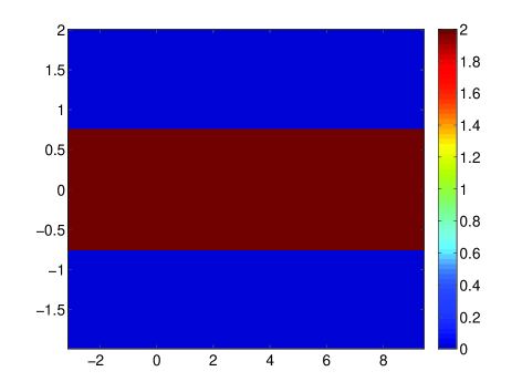
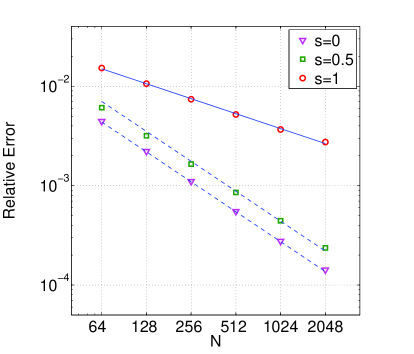
(a)	(b)

Figure 3: (a) Two periods (in the horizontal variable) of the strip structure with contrast equal to two. (b) Relative error between the numerically approximated solution and the analytically computed reference solution measured in $H^{s}_{\mathrm{per}}$-norm for scattering from the strip shown in (a). Circles, kites, triangles correspond to $s=1$, $s=0.5$ and $s=0$, respectively. The continuous line and the dotted lines indicate the convergence order 0.5 and 1, respectively. The discretization parameter is $N=2^{n}$ for $n=6,...,11$.

$N$ 64 128 256 512 1024 2048 Computation time(s) for strip-structure 0.3 1.1 3.7 21.2 131.7 463.7 $\sharp$ GMRES iterations for strip-structure 7 6 6 6 6 5

Table 1: Computation times and number of GMRES iterations for the computation of the errors for the simple strip structure shown in Figure 3. The parameter $N$ is the discretization parameter of the trigonometric Galerkin scheme.

Of course, the numerical results for the strip structure from the last example merely provide a first test that the algorithm computes correct solutions. For further tests and illustrations of the algorithm, we consider more complicated structures where the contrast varies smoothly within subdomains and jumps across subdomain borders. As we mentioned in the introduction and confirmed in Lemma 4.3, it is essential for the Galerkin scheme to have explicit values of the Fourier coefficients $\hat{q}_{2N}$ of the contrast $q$ at hand. In principle, these values could be approximated using FFTs. However, we found that whenever one is able to compute these Fourier coefficients analytically, this results in considerably more accurate computations. In the examples below, we explain case-by-case how to compute these Fourier coefficients for a wide class of polynomially or exponentially varying materials. For complicated material shapes, it is usually impossible to compute the Fourier coefficients explicitly. Using partial integrations, one is however able to come up with semi-analytic expressions that merely require a one-dimensional integration of a periodic and piecewise analytic function for evaluation.

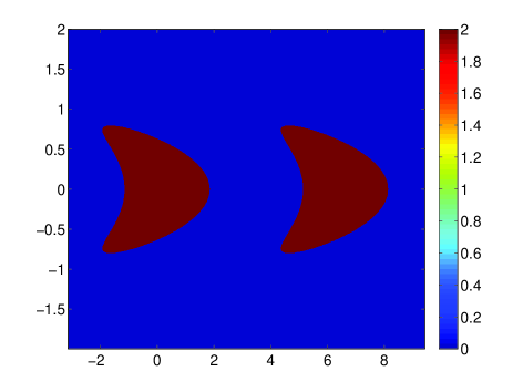
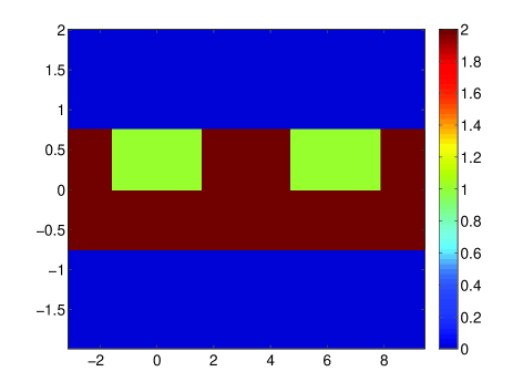
(a)	(b)
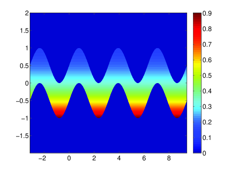
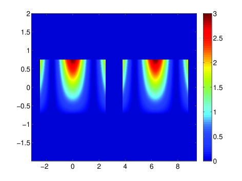
(c)	(d)

Figure 4: The four plots show two periods in the horizontal variable of the contrasts $q_{1,2,3,4}$ considered in the numerical experiments below. (a) The piecewise constant kite-shaped contrast $q_{1}$. (b) The piecewise constant contrast $q_{2}$ is supported in a strip. (c) The contrast $q_{3}$ varies smoothly within a sinusoidally-shaped strip. (d) The contrast $q_{4}$ varies smoothly within a rectangle.

Figure 4 shows the four contrasts $q_{1,2,3,4}$ that we consider in the experiments below. We start now by giving precise definitions of these four contrasts and we compute their Fourier coefficients (semi-)explicitly. Afterwards, we present numerical examples for the different structures. We would like to point out in advance that for all four examples the domain $\Omega_{R}$ will be chosen as $(-\pi,\pi)\times(-2,2)$, i.e., $R=2$ always.

The contrast $q_{1}$ plotted in Figure 4(a) consists of $2\pi$-periodically aligned kite-shaped inclusions with constant material parameter (the contrast equals to two inside the inclusion). The boundary of the central inclusion $D\subset(-\pi,\pi)\times(-2,2)$ is parametrized by $t\mapsto(1.5\cos(t)+\cos(2t)-0.65,\sin(t))^{\top},\ t\in[0,2\pi]$. The Fourier coefficients $\{\hat{q}_{1}(j)\}_{j\in\mathbb{Z}^{2}}$ can simply be computed using Green’s formula,

$$\sqrt{8\pi}\ \hat{q}_{1}(j) =\int_{\Omega_{R}}q(x)e^{-\mathrm{i}j_{1}x_{1}-\mathrm{i}\frac{j_{2}\pi}{2}x_{2}}\,\mathrm{d}x\,$$

$$=2\int_{D}e^{-\mathrm{i}j_{1}x_{1}-\mathrm{i}\frac{j_{2}\pi}{2}x_{2}}\,\mathrm{d}x\,=\frac{4\mathrm{i}}{j_{2}\pi}\int_{\partial D}\nu_{2}(x)e^{-\mathrm{i}j_{1}x_{1}-i\frac{j_{2}\pi}{2}x_{2}}\,\mathrm{d}s\,$$

$$=\frac{4\mathrm{i}}{j_{2}\pi}\int_{0}^{2\pi}e^{-\mathrm{i}j_{1}z_{1}(t)-\mathrm{i}\frac{j_{2}\pi}{2}\sin(t)}(1.5\sin(t)+2\sin(2t))\,\mathrm{d}t\,,\quad j_{2}\neq 0.$$

This integral can now be accurately evaluated numerically (we use the fourth-order convergent composite Simpson’s rule).

Similar techniques yield the Fourier coefficients of the contrast

$$q_{2}=\begin{cases}1&\text{ in }D_{1}:=(-\pi/2,\pi/2)\times(0,0.75),\\ 2&\text{ in }(-\pi,\pi)\times(-0.75,0.75)\setminus\overline{D_{1}},\end{cases}$$

that is plotted in Figure 4(b). The Fourier coefficients of $q_{2}$ can be computed explicitly,

$$\sqrt{8\pi}\ \hat{q}_{2}(j) =-\int_{D_{1}}e^{-\mathrm{i}j_{1}x_{1}-\mathrm{i}j_{2}\pi x_{2}/2}\,\mathrm{d}x\,+2\int_{D}e^{-\mathrm{i}j_{1}x_{1}-\mathrm{i}j_{2}\pi x_{2}/2}\,\mathrm{d}x\,,\quad j\in\mathbb{Z}^{2}.$$

Both integrals can of course be computed analytically, the first one equals for instance $4\mathrm{i}/(\pi j_{1}j_{2})\,\sin(j_{1}\pi/2)[1-\exp(-3/8\,\pi\mathrm{i}j_{1})]$ for $j_{1,2}\not=0$.

The contrast $q_{3}$ shown in Figure 4(c) is defined as a smooth function on a sinusoidally shaped strip $D$. In detail,

$$D =\big{\{}\left(\begin{smallmatrix}x_{1}\\ x_{2}\end{smallmatrix}\right)\in\mathbb{R}^{2}:\ -\pi<x_{1}<\pi,\ \sin(2x_{1})<2x_{2}-1<\sin(2x_{1})\big{\}}\quad\text{and }\quad$$

$$q_{3}(x) =\begin{cases}e^{-x_{2}}/3&\text{for }x=\left(\begin{smallmatrix}x_{1}\\ x_{2}\end{smallmatrix}\right)\in D,\\ 0&\text{else}.\end{cases}$$

In this case the Fourier coefficients of the contrast $q$ can be computed semi-analytically using Green’s formula

$$\sqrt{8\pi}\ \hat{q}_{3}(j) =\int_{\Omega_{R}}q(x)e^{-\mathrm{i}j_{1}x_{1}-\mathrm{i}j_{2}\pi x_{2}/2}\,\mathrm{d}x\,=\frac{1}{3}\int_{D}e^{-\mathrm{i}j_{1}x_{1}-(1+\mathrm{i}j_{2}\pi/2)x_{2}}\,\mathrm{d}x\,$$

$$=\frac{-1/3}{1+\mathrm{i}j_{2}\pi/2}\int_{\partial D}\nu_{2}(x)e^{-\mathrm{i}j_{1}x_{1}-(1+\mathrm{i}j_{2}\pi/2)x_{2}}\,\mathrm{d}s\,$$

$$=\frac{-1/3}{1+\mathrm{i}j_{2}\pi/2}\int_{0}^{2\pi}e^{-\mathrm{i}j_{1}t-(1+\mathrm{i}j_{2}\pi/2)(\sin(2t)/2+1/2)}\,\mathrm{d}t\,$$

$$\quad+\frac{1/3}{1+\mathrm{i}j_{2}\pi/2}\int_{0}^{2\pi}e^{-\mathrm{i}j_{1}t-(1+\mathrm{i}j_{2}\pi/2)(\sin(2t)/2-1/2)}\,\mathrm{d}t\,.$$

Again, we approximate these integrals with the fourth-order convergent composite Simpson’s rule to get accurate approximations for the Fourier coefficients of $q_{3}$.

Remark 5.1.

Of course, a similar integration-by-parts trick with respect to $x_{1}$ would still work if $q_{3}$ depends in a more complicated way on $x_{2}$. This shows that in principle the Fourier coefficients of contrasts that vary smoothly in one variable can be computed by approximating one-dimensional integrals of smooth functions.

Finally, we define the contrast function $q_{4}$ plotted in Figure 4(d) – a contrast function that varies smoothly in a $2\pi$-periodic rectangle-shaped structure with support $\overline{D}$, $D=(-2.5,2.5)\times(-0.75,0.75)$. In detail,

$$q_{4}(x)=2\cos(x_{1})^{2}(x_{2}+0.75)\quad\text{for }x=(x_{1},x_{2})^{\top}\in D$$

and $q_{4}(x)=0$ for points outside of $D$. The Fourier coefficients of $q_{4}$ can be explicitly computed using integration-by-parts techniques we already used above. Omitting technical details, the result is that

$$\hat{q}(j)=\frac{A(j_{1})B(j_{2})}{\sqrt{8\pi}}\quad\text{for }j=(j_{1},j_{2})^{\top}\in\mathbb{Z}^{2},$$

where

$$A(j_{1}) =\begin{cases}\frac{\sin(5j_{1})\big{[}(2\cos(10)+1)/{j_{1}}-8/{j_{1}^{3}}\big{]}-4\cos(5j_{1})\sin(10)/{j_{1}^{2}}}{1-4/{j_{1}^{2}}}&j_{1}\in\mathbb{Z}\setminus\{0,\pm 2\},\\ \sin(20)/4+\sin(10)+5&j_{1}=\pm 2,\\ \sin(10)/2+5&j_{1}=0,\end{cases}$$

$$B(j_{2}) =\begin{cases}\frac{6\mathrm{i}}{j_{2}\pi}\exp(-3\pi\mathrm{i}j_{2}/4)-\frac{8\mathrm{i}}{(j_{2}\pi)^{2}}\sin(3\pi j_{2}/4)&j_{2}\neq 0,\\ 9/2&j_{2}=0.\end{cases}$$

Remark 5.2.

The last example shows that Fourier coefficients of contrasts of the form $q(x)=f_{1}(x_{1})f_{2}(x_{2})$ can be computed (semi-)analytically if $f_{1,2}$ are trigonometric functions, exponentials, or polynomials. The last example features a linear function $f_{2}(x_{2})=x_{2}+0.75$, however, higher-degree polynomials could be treated as well using additional integrations by parts reducing the polynomial degree.

Since explicit analytic solutions for plane wave scattering problems involving the contrast functions $q_{1,2,3,4}$ are not known, we check convergence rates for these structures by computing a reference solution for very large discretization parameter $N$. For all examples below, this reference solution is computed for $N=3072$ using GMRES with a relative residual reduction factor of $10^{-8}$. The angle of the incident plane wave is always chosen as $\theta=\pi/4$ and the wave number always equals $k=\pi/2$. We check the convergence rates from Proposition 4.1 by computing scattered fields for discretization parameter $N=2^{n}$, $n=4,\dots,9$. As above, the GMRES algorithm is stopped when the relative residual reduction factor is less than $10^{-5}$. Figure 5 shows that the convergence order of the method in the energy norm $H^{1}_{\mathrm{per}}$ is in good agreement with the statement of Proposition 4.1. Further, for all test cases, the rates of the error measured in $H^{1/2}_{\mathrm{per}}$ and in $L^{2}$ are in good agreement with the statement of Remark 4.2. Computation times and the number of iterations of the GMRES algorithm corresponding to the numerical experiments illustrated in Figure 5 are shown in Table 2.

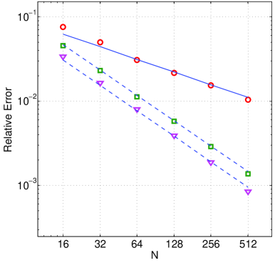
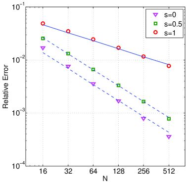
(a)	(b)
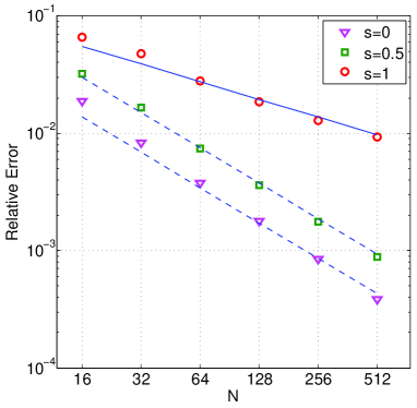
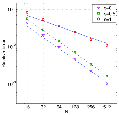
(c)	(d)

Figure 5: Test for the convergence rate of the trigonometric Galerkin discretization for the different structures presented in Figure 4. The plots show the relative error in the $H^{s}_{\alpha,\mathrm{per}}$-norm between the approximate solution ($N=2^{n}$, $n=4,\dots,9$) and the reference solution ($N=3072$), plotted against the discretization parameter $N$. Circles, kites, triangles correspond to $s=1$, $s=0.5$ and $s=0$, respectively. The continuous line and the dotted lines indicate the expected convergence orders 0.5 and 1, respectively. (a) Results for the kite-shaped contrast $q_{1}$ from Figure 4(a). (b) Results for the piecewise constant contrast $q_{2}$ from Figure 4(b). (c) Results for the contrast $q_{3}$ that varies smoothly within a sinusoidal strip from Figure 4(c). (d) Results for the contrast $q_{4}$ that varies smoothly within a rectangle from Figure 4(d).

$N$ 64 128 256 512 Time(s) for $q_{1}$ (Figure 4(a)) 1.4 7 44 295 Time(s) for $q_{2}$ (Figure 4(b)) 1.7 5 16 47 Time(s) for $q_{3}$ (Figure 4(c)) 1.6 7 39 184 Time(s) for $q_{4}$ (Figure 4(d)) 0.4 2 8 39 $\sharp$ GMRES iterations for $q_{1}$ (Figure 4(a)) 10 11 11 11 $\sharp$ GMRES iterations for $q_{2}$ (Figure 4(b)) 12 12 12 12 $\sharp$ GMRES iterations for $q_{3}$ (Figure 4(c)) 6 6 6 6 $\sharp$ GMRES iterations for $q_{4}$ (Figure 4(c)) 9 10 10 10

Table 2: Computation times and number of GMRES iterations for the computation of the error curves shown in Figure 5. Computing the reference solutions took roughly 1 hour for $q_{2}$ and $q_{4}$, 10 hours for $q_{3}$ and 16 hours for $q_{1}$.

The last computational experiment illustrates the convergence of the trigonometric Galerkin technique using an error indicator resulting from energy conservation. Recall the Rayleigh coefficients $\hat{u}^{\pm}_{j}$ of the scattered field from (4). For the incident plane wave $u^{i}$ with incident angle $\theta$, we define similar coefficients by $\hat{u}^{i}_{j}=\int_{-\pi}^{\pi}u^{i}(x_{1},-h)\exp(-\mathrm{i}\alpha_{j}x_{1})\,\mathrm{d}x_{1}\,$ for $j\in\mathbb{Z}$. Then Green’s formula applied to equation (1) together with the Rayleigh expansion condition shows that

$$\sum_{j:k^{2}>\beta_{j}^{2}}\beta_{j}(|\hat{u}^{+}_{j}|^{2}+|\hat{u}^{-}_{j}+\hat{u}^{i}_{j}|^{2})=\beta_{0}.$$ (24)

The sums

$$E_{\mathrm{tra}}(\theta):=\sum_{j:k^{2}>\beta_{j}^{2}}\beta_{j}(|\hat{u}^{-}_{j}+\hat{u}^{i}_{j}|^{2})/\beta_{0},\qquad E_{\mathrm{ref}}(\theta):=\sum_{j:k^{2}>\beta_{j}^{2}}\beta_{j}|\hat{u}^{+}_{j}|^{2}/\beta_{0}$$

correspond to transmitted and reflected wave energies. In the following experiment, we compute the function

$$\theta\mapsto|1-E_{\mathrm{tra}}(\theta)-E_{\mathrm{ref}}(\theta)|$$ (25)

for many angles $\theta$ to obtain an error indicator for the numerical accuracy of the integral equation solver in dependence on the angle of the incident field. This angle, $\theta$, is sampled at 200 points uniformly distributed in the interval $[0.2,1.2]$. The wave number $k$ equals 2.5. To compute the energy curves shown in Figure 6(a) the scattered field is approximated in $\mathcal{T}_{N}$ where $N=2^{8}=256$. The relative residual reduction factor for the GMRES iteration is in this experiment always chosen as $10^{-8}$. With this choice, the computation time for solving for one fixed incident angle $\theta$ is about 8 seconds. In Figure 6(b) we check the error indicator of energy conservation from (25) for different discretization parameters $N$. This plot shows that the error of the computed Rayleigh coefficients corresponding to propagating modes converges with order 1, exactly as the error of the solutions in $H^{1/2}_{\mathrm{per}}$. This seems natural since, first, the Rayleigh coefficients are obtained from the numerical solution $u_{N}$ by integration over the line $\Gamma_{\rho}=(-\pi,\pi)\times\{\rho\}$ and, second, the trace theorem states that the mapping $u_{N}\mapsto\left.u_{N}\right|_{\Gamma_{\rho}}$ is bounded from $H^{s}_{\mathrm{per}}(\Omega_{R})$ into $L^{2}(\Gamma_{\rho})$ for $s>1/2$. The plot in Figure 6(b) further shows a slight instability around a Wood’s anomaly at the angle $\theta=\arccos(1-1/(2.5))\approx 0.927$, as it is going to be expected from Remark 2.1. (The sampling points naturally avoid the exact value of the angle corresponding to this Wood’s anomaly.)

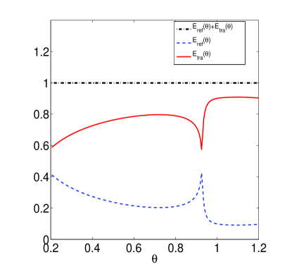
(a)

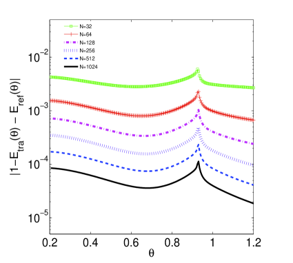
(b)

Figure 6: (a) Reflected energy curves (low dashed line) and transmitted energy curves (continuous line) plotted against the angle $\theta$ of the incident plane wave $u^{i}$. The two curves sum up to one, as they should due to (24). (b) The error criterion (25) plotted for different discretization parameters $N=2^{n}$, $n=5,\dots,10$, versus the angle $\theta$ of the incident plane wave. (The order of the curves from top to bottom corresponds to the increasing discretization parameter $N$.)