Model-independent Study of Electric Dipole Transitions in Quarkonium

Abstract

The paper contains a systematic, model-independent treatment of electric dipole (E1) transitions in heavy quarkonium. Within the effective field theory framework of potential non-relativistic QCD (pNRQCD), we derive the complete set of relativistic corrections of relative order $v^{2}$ both for weakly and strongly-coupled quarkonia. The result supports and complements former results from potential model calculations.

I Introduction

In recent years, BES, the B-factories and CLEO have improved on almost all heavy-quarkonium radiative transition modes and measured many of them for the first time. Part of this impressive progress can be found collected in two reviews by the Quarkonium Working Group Brambilla:2004wf ; arXiv:1010.5827 . Among the most recent developments we mention the first measurements of $h_{c}\rightarrow\eta_{c}\,\gamma$ by BES arXiv:1002.0501 , $\Upsilon(2S)\rightarrow\eta_{b}\,\gamma$ by BABAR arXiv:0903.1124 , $\Upsilon(3S)\rightarrow\eta_{b}\,\gamma$ by CLEO arXiv:0909.5474 , $h_{b}\rightarrow\eta_{b}\,\gamma$ by BABAR and BELLE arXiv:1102.4565 , and the measurements of the branching fractions for electromagnetic transitions of the $\chi_{b}$ states by CLEO arXiv:1012.0589 and BABAR arXiv:1104.5254 .

Electric dipole (E1) transitions are transitions that change the orbital angular momentum of the state by one unit, but not its spin. Hence, the final state has a different parity and C parity than the initial one. Typical E1 transitions are $n^{\prime\,3}P_{J}\rightarrow n^{3}S_{1}\,\gamma$, e.g. $\chi_{cJ}\rightarrow J/\psi\,\gamma$ or $\chi_{bJ}\rightarrow\Upsilon(1S)\,\gamma$, and $n^{\prime\,1}P_{1}\rightarrow n^{1}S_{0}\,\gamma$, e.g. $h_{c}\rightarrow\eta_{c}\,\gamma$ or $h_{b}\rightarrow\eta_{b}\,\gamma$. E1 transitions happen more frequently than magnetic dipole (M1) transitions. The branching fraction of E1 transitions can indeed be quite significant for some states, e.g. the branching fraction for $\chi_{b1}\rightarrow\Upsilon(1S)\,\gamma$ is $(35\pm 8)\%$ and the branching fraction for $\chi_{b2}\rightarrow\Upsilon(1S)\,\gamma$ is $(22\pm 4)\%$ FERMILAB-PUB-10-665-PPD . E1 transitions depend on the wave function already at leading order and therefore provide a direct insight into the quarkonium state.

Electromagnetic transitions have been treated for a long time by means of potential models using non-relativistic reductions of phenomenological interactions (see e.g. PRINT-84-0308 , which will be our reference work in the field). A recent comprehensive analysis can be found in hep-ph/0701208 . However the progress made in effective field theories (EFTs) for non-relativistic systems, like quarkonium, hep-ph/0410047 , and the new large set of accurate data ask for model-independent analyses. M1 transitions have been treated in an EFT framework in hep-ph/0512369 . In this work, we extend that previous analysis to E1 transitions, for which a model-independent treatment has been missing so far.

Effective field theories for quarkonium radiative transitions are built on a hierarchy of energy scales hep-ph/0512369 : the heavy-quark mass $m$, the relative momentum of the bound state $p\sim mv$ and the binding energy $E\sim mv^{2}$, where $v\ll 1$ is the heavy-quark velocity in the center of mass frame. The condition $v\ll 1$, which works better for bottomonium ($v_{b}^{2}\approx 0.1$) than for charmonium ($v_{c}^{2}\approx 0.3$), implies $m\gg p\gg E$. For transitions that involve a change in the principal quantum number, the photon energy, $k_{\gamma}$, scales like $k_{\gamma}\sim mv^{2}$. This counting will be assumed throughout the paper, although, for transitions between states with the same principal quantum number, the photon energy is smaller. A smaller photon energy may be implemented easily in the final expressions of the transition widths by suppressing terms proportional to $k_{\gamma}$ accordingly. Observables like the transition widths are organized in an expansion in $v^{2}$; the main purpose of the paper is to provide, in an EFT framework, an expression for E1 transition widths valid up to relative order $v^{2}$. The work is partially based on Piotr .

The paper is organized as follows. In Sec. II, we construct the EFT Lagrangian relevant for E1 decays up to relative order $v^{2}$. The matching is performed in Sec. III. In Sec. IV, we set up the calculation of the transition rates. In Sec. V, we calculate the relativistic corrections and, in Sec. VI, we write the widths up to order $v^{2}$. There we also compare our results with those in PRINT-84-0308 . Finally, in Sec. VII, we conclude and discuss future applications.

II Effective Field Theories

In this section, we write the low-energy EFT suited to describe E1 electromagnetic transitions in heavy quarkonia. The EFT is constructed in two steps. The first step consists of integrating out modes associated with the scale $m$. This leads to non-relativistic QCD (NRQCD) coupled to electromagnetism CLNS-85/641 ; hep-ph/9407339 . The second step consists of integrating out modes associated with the scale $mv$, which leads to potential non-relativistic QCD (pNRQCD) hep-ph/9707481 ; hep-ph/9907240 . The operators of pNRQCD relevant for M1 transitions have been derived in hep-ph/0512369 ; here we consider the electromagnetic operators responsible for E1 transitions.

The EFT matrix elements are counted in powers of $v$, while the Wilson coefficients of NRQCD are series in $\alpha_{\textrm{s}}$ at the (perturbative) mass scale. Heavy quarkonia may be distinguished in weakly-coupled and strongly-coupled quarkonia. For weakly-coupled quarkonia, the binding energy is of the order of or larger than the typical hadronic scale $\Lambda_{\textrm{QCD}}$. This case may be relevant for bottomonium and charmonium ground states. Weakly-coupled quarkonia can be treated perturbatively at the typical momentum-transfer scale leading to a potential that is Coulombic. The heavy-quark velocity is of order $\alpha_{\textrm{s}}$ and we may identify the momentum-transfer scale with $m\alpha_{\textrm{s}}$ and the binding-energy scale with $m\alpha_{\textrm{s}}^{2}$. The Wilson coefficients of weakly-coupled pNRQCD are series in $\alpha_{\textrm{s}}$, which can be obtained by expanding in $\alpha_{\textrm{s}}$ when matching pNRQCD to NRQCD. We will see, however, that, for E1 operators contributing to the transition widths up to relative order $v^{2}$, such an expansion is not necessary and the obtained results will be valid to all orders in the coupling. In the most general weakly-coupled case, the binding energy is not a perturbative scale, $m\alpha_{\textrm{s}}^{2}\sim\Lambda_{\textrm{QCD}}$, and $\alpha_{\textrm{s}}$ at that scale may not be considered an expansion parameter.

For strongly-coupled quarkonia, $\Lambda_{\textrm{QCD}}$ is larger than the binding energy and possibly of the same order as the momentum transfer. This case may be relevant for all higher bottomonium and charmonium states. Since E1 transitions require that at least one involved quarkonium state has principal quantum number larger than one, strongly-coupled quarkonia are likely to be always involved in such processes. Strongly-coupled quarkonia may in general not be treated perturbatively at the typical momentum-transfer scale. This leads, in particular, to a potential that is not Coulombic.

II.1 NRQCD

We consider NRQCD coupled to electromagnetism. The Lagrangian has the form

$$\mathcal{L}_{\textrm{NRQCD}}=\mathcal{L}_{\textrm{2-f}}+\mathcal{L}_{\textrm{4-f}}+\mathcal{L}_{\textrm{light}}\,.$$ (1)

The term $\mathcal{L}_{\textrm{2-f}}$ denotes the two-fermion sector of the Lagrangian. If we restrict ourselves to operators relevant for E1 transition widths up to relative order $v^{2}$, $\mathcal{L}_{\textrm{2-f}}$ reads

$${\cal L}_{\textrm{2-f}} = \psi^{\dagger}\left(iD_{0}+\frac{{\bf D}^{2}}{2m}+\frac{{\bf D}^{4}}{8m^{3}}\right)\psi$$ (2)

$$+\frac{c_{F}}{2m}\psi^{\dagger}{\mbox{\boldmath$\sigma$}}\cdot g{\bf B}\psi-\frac{c_{S}}{8m^{2}}\psi^{\dagger}\mbox{\boldmath$\sigma$}\cdot[-i{\bf D}\times,g{\bf E}]\psi+\frac{c_{D}}{8m^{2}}\psi^{\dagger}\left[{\bf D}\cdot,g{\bf E}\right]\psi$$

$$+\frac{c_{F}^{\textrm{em}}}{2m}\psi^{\dagger}\mbox{\boldmath$\sigma$}\cdot ee_{Q}{\bf B}^{{\textrm{em}}}\psi-\frac{c_{S}^{\textrm{em}}}{8m^{2}}\psi^{\dagger}\mbox{\boldmath$\sigma$}\cdot[-i{\bf D}\times,ee_{Q}{\bf E}^{{\textrm{em}}}]\psi+\frac{c_{D}^{\textrm{em}}}{8m^{2}}\psi^{\dagger}\left[{\bf D}\cdot,g{\bf E}^{{\textrm{em}}}\right]\psi$$

$$+[\psi\rightarrow i\sigma^{2}\chi^{*},A_{\mu}\rightarrow-A_{\mu}^{T},A^{{\textrm{em}}}_{\mu}\rightarrow-A^{{\textrm{em}}}_{\mu}]\,,$$

where $\psi$ is the Pauli spinor field that annihilates a heavy quark of mass $m$, flavor $Q$ and electric charge $ee_{Q}$ ($e_{b}=-1/3$, $e_{c}=2/3$), and $\chi$ is the corresponding Pauli spinor that creates a heavy antiquark. The gauge fields with superscript “em” are the electromagnetic fields, the others are gluon fields, $iD_{0}=i\partial_{0}-gT^{a}A^{a}_{0}-ee_{Q}A^{{\textrm{em}}}_{0}$, $i{\bf D}=i\mbox{\boldmath$\nabla$}+gT^{a}{\bf A}^{a}+ee_{Q}{\bf A}^{{\textrm{em}}}$, $[{\bf D}\times,{\bf E}]={\bf D}\times{\bf E}-{\bf E}\times{\bf D}$, ${\bf E}^{i}=F^{i0}$, ${\bf B}^{i}=-\epsilon_{ijk}F^{jk}/2$, ${\bf E}^{i\,{\textrm{em}}}=F^{i0\,{\textrm{em}}}$ and ${\bf B}^{i\,{\textrm{em}}}=-\epsilon_{ijk}F^{jk\,{\textrm{em}}}/2$.

The coefficients $c_{F}$, $c_{S}$, $c_{D}$, $c_{F}^{{\textrm{em}}}$, $c_{S}^{{\textrm{em}}}$ and $c_{D}^{{\textrm{em}}}$ are Wilson coefficients of NRQCD. Some of them satisfy exact relations dictated by reparameterization (or Poincaré) invariance hep-ph/9205228 , e.g.

$$c_{S}^{{\textrm{em}}} = 2c_{F}^{{\textrm{em}}}-1\,,\qquad c_{S}=2c_{F}-1\,.$$ (3)

The coefficients are one at leading order, but known at least at one loop hep-ph/9701294 . In particular, we have

$$c_{F}^{{\textrm{em}}}\equiv 1+\kappa_{Q}^{{\textrm{em}}} = 1+C_{F}\frac{\alpha_{\textrm{s}}}{2\pi}+{\cal O}(\alpha_{\textrm{s}}^{2})\,,$$ (4)

where $C_{F}=(N_{c}^{2}-1)/(2N_{c})=4/3$ and $N_{c}=3$. The term $\kappa_{Q}^{{\textrm{em}}}$ is usually identified with the anomalous magnetic moment of the heavy quark $Q$; $\kappa_{Q}^{{\textrm{em}}}$ is less than $0.1$ for charm and bottom. In general, the Wilson coefficients of NRQCD contain also contributions coming from virtual photons of energy or momentum of order $m$. These contributions are suppressed by powers of $\alpha$, the fine structure constant, and will be neglected in the following.

The terms $\mathcal{L}_{\textrm{4-f}}$ and $\mathcal{L}_{\textrm{light}}$ denote respectively the four-fermion sector and the light-field sector of the Lagrangian. Light fields include light quarks (assumed to be massless), charm quarks in the bottomonium case, gluons and photons. $\mathcal{L}_{\textrm{4-f}}$ and $\mathcal{L}_{\textrm{light}}$ contribute to the quarkonium potential and wave functions (see hep-ph/0410047 and references therein), but they do not provide new couplings of the heavy quarks with the electromagnetic fields relevant for E1 transitions at relative order $v^{2}$, which is the accuracy we aim at.

II.2 pNRQCD

In NRQCD, degrees of freedom that scale with the momentum transfer and with the binding energy are entangled in physical amplitudes, leading to a non-homogeneous power counting. These degrees of freedom are disentangled in pNRQCD, where degrees of freedom that scale like $mv$ have been integrated out. The pNRQCD Lagrangian may be decomposed in two terms:

$$\mathcal{L}_{\textrm{pNRQCD}}=\mathcal{L}_{\textrm{0}}+\mathcal{L}_{\gamma\textrm{pNRQCD}}\,.$$ (5)

The term $\mathcal{L}_{\textrm{0}}$ denotes the part of the pNRQCD Lagrangian that does not contain heavy-quark couplings to electromagnetism. In its gauge-invariant form, it reads

$$\mathcal{L}_{\textrm{0}}=\int d^{3}r\;\mathrm{Tr}\left\{\mathrm{S}^{\dagger}\left({i{\partial}_{0}+\frac{{\boldsymbol{\nabla}}^{2}}{4m}+\frac{{\boldsymbol{\nabla}}_{r}^{2}}{m}+\frac{{\boldsymbol{\nabla}}_{r}^{4}}{4m^{3}}}+\dots-V_{S}\right)\mathrm{S}\right\}+\Delta\mathcal{L}_{\textrm{0}}\,,$$ (6)

where ${\rm S}=S1\!\!{\rm l}_{c}/\sqrt{N_{c}}$ is a quark-antiquark field that transforms as a singlet under $SU(3)_{\rm c}$ and $U(1)_{{\textrm{em}}}$. $S$ is labeled by the quark-antiquark distance ${\bf r}$ and depends on the center of mass coordinate and time, the derivative $\nabla$ acts on the center of mass coordinate and the derivative $\mbox{\boldmath$\nabla$}_{r}$ on the relative distance ${\bf r}$. The dots stand for higher-order kinetic energy terms. Here and in the following, the trace is meant over color and spin indices. The Wilson coefficient $V_{S}$, which is in general a function of ${\bf r}$, may be identified with the quark-antiquark color-singlet potential. It is organized as an expansion in $1/m$, the leading term being the static potential, $V_{S}^{(0)}$. For weakly-coupled quarkonia, $V_{S}$ may be calculated in perturbation theory, the leading term being the Coulomb potential ($V_{S}^{(0)}=-C_{F}\alpha_{\textrm{s}}/r$). For strongly-coupled quarkonia, $V_{S}$ follows from a non-perturbative matching to NRQCD.

The term $\Delta\mathcal{L}_{\textrm{0}}$ describes the propagation of all other low-energy degrees of freedom besides the quark-antiquark singlet and their strong interactions. The low-energy degrees of freedom depend on the specific quarkonium under scrutiny. For weakly-coupled quarkonia, they are, besides the quark-antiquark singlet field, the quark-antiquark field ${\rm O}=\sqrt{2}\,O^{a}T^{a}$, which transforms as an octet under $SU(3)_{\rm c}$ and as a singlet under $U(1)_{{\textrm{em}}}$, light quarks, low-energy gluons and photons; $\Delta\mathcal{L}_{\textrm{0}}$ then reads

$$\Delta\mathcal{L}_{\textrm{0}} = \int d^{3}r\;\mathrm{Tr}\Bigg{\{}\mathrm{O}^{\dagger}\left({iD_{0}+\frac{{\boldsymbol{D}}^{2}}{4m}+\frac{{\boldsymbol{\nabla}}_{r}^{2}}{m}}+\dots-V_{O}\right)\mathrm{O}$$ (7)

$$\hskip 56.9055pt+V_{A}\left(\mathrm{O}^{\dagger}{\bf r}\cdot g{\bf E}\mathrm{S}+\mathrm{S}^{\dagger}{\bf r}\cdot g{\bf E}\mathrm{O}\right)+\dots\Bigg{\}}+\mathcal{L}_{\textrm{light}}\,,$$

where $iD_{0}\mathrm{O}=i\partial_{0}\mathrm{O}-g[T^{a}A_{0}^{a},\mathrm{O}]$ and $i{\bf D}\mathrm{O}=i\boldsymbol{\nabla}\mathrm{O}+g[T^{a}{\bf A}^{a},\mathrm{O}]$. Like $S$, the fields $O^{a}$ are labeled by the quark-antiquark distance ${\bf r}$ and depend on the center of mass coordinate and time. To ensure that gluons and photons are of low-energy (i.e. carry energy and momentum lower than the typical momentum transfer in the quark-antiquark system) gluon and photon fields are multipole expanded in the relative distance ${\bf r}$ and depend only on the center of mass coordinate and time. Hence the Lagrangian is organized as an expansion in ${\bf r}$ and $1/m$ (inherited from NRQCD). The dots in (7) stand for terms that contribute to E1 transitions beyond our accuracy. The Wilson coefficient $V_{O}$ may be identified with the quark-antiquark color-octet potential. It is organized as an expansion in $1/m$, the leading term being the static potential, $V_{O}^{(0)}$. At leading order in perturbation theory, $V_{O}^{(0)}=\alpha_{\textrm{s}}/(2N_{c}r)$. The Wilson coefficient $V_{A}=1+{\cal O}(\alpha_{\textrm{s}}^{2})$ Brambilla:2009bi provides the strength of the chromoelectric dipole interaction. $\mathcal{L}_{\textrm{light}}$ denotes the light-field sector of the Lagrangian; light fields include light quarks (assumed to be massless), gluons and photons. For strongly-coupled quarkonia, after having integrated out $\Lambda_{\textrm{QCD}}$, only degrees of freedom that are color singlet are possible hep-ph/0002250 ; hep-ph/0009145 . These are, besides the quark-antiquark color-singlet field and photons, the Goldstone bosons associated to the spontaneous breaking of chiral symmetry. The effects of Goldstone bosons on E1 transitions go beyond our accuracy and will be neglected. Hence, for strongly-coupled quarkonia we set $\Delta\mathcal{L}_{\textrm{0}}=-F_{\mu\nu}^{{\textrm{em}}}F^{\mu\nu\,{{\textrm{em}}}}/4$, whereas all the complication of the non-perturbative treatment goes in the determination of $V_{S}$.

The term $\mathcal{L}_{\gamma\textrm{pNRQCD}}$ describes the coupling of heavy quark-antiquark pairs with low-energy photons, like those responsible for electromagnetic transitions. The power counting goes as follows

$$r\sim 1/mv,\quad\mbox{\boldmath$\nabla$}_{r}\sim mv,\quad\mbox{\boldmath$\nabla$}\sim mv^{2},k_{\gamma},\quad{\bf E}^{{\textrm{em}}},{\bf B}^{{\textrm{em}}}\sim k_{\gamma}^{2}\,;$$ (8)

in the case of weakly-coupled quarkonia, one has to consider also low-energy gluons that scale with $mv^{2}$ or $k_{\gamma}$. The leading operator responsible for E1 transitions is the electric dipole operator $\mathrm{S}^{\dagger}{\bf r}\cdot ee_{Q}{\bf E}^{{\textrm{em}}}\mathrm{S}$, while operators relevant for E1 transitions at relative order $v^{2}$ are those suppressed by $v^{2}$ with respect to it. The part of $\mathcal{L}_{\gamma\textrm{pNRQCD}}$ relevant for E1 transitions is (operators relevant for M1 transitions have been listed in hep-ph/0512369 )

$$\mathcal{L}_{\gamma\textrm{pNRQCD}}=\int d^{3}r\;\mathrm{Tr} \Bigg{\{}V^{r\cdot E}\mathrm{S}^{\dagger}{\bf r}\cdot ee_{Q}{\bf E}^{{\textrm{em}}}\mathrm{S}$$

$$+\frac{1}{24}V^{(r\nabla)^{2}r\cdot E}\mathrm{S}^{\dagger}{\bf r}\cdot[({\bf r}\cdot\mbox{\boldmath$\nabla$})^{2}ee_{Q}{\bf E}^{{\textrm{em}}}]\mathrm{S}$$

$$+\frac{i}{4m}V^{\nabla\cdot(r\times B)}\mathrm{S}^{\dagger}\{\mbox{\boldmath$\nabla$}\cdot,{\bf r}\times ee_{Q}{\bf B}^{{\textrm{em}}}\}\mathrm{S}$$

$$+\frac{i}{12m}V^{\nabla_{r}\cdot(r\times(r\nabla)B)}\mathrm{S}^{\dagger}\{\mbox{\boldmath$\nabla$}_{r}\cdot,{\bf r}\times[({\bf r}\cdot\mbox{\boldmath$\nabla$})ee_{Q}{\bf B}^{{\textrm{em}}}]\}\mathrm{S}$$

$$+\frac{1}{4m}V^{(r\nabla)\sigma\cdot B}[\mathrm{S}^{\dagger},\mbox{\boldmath$\sigma$}]\cdot[({\bf r}\cdot\mbox{\boldmath$\nabla$})ee_{Q}{\bf B}^{{\textrm{em}}}]\mathrm{S}$$

$$-\frac{i}{4m^{2}}V^{\sigma\cdot(E\times\nabla_{r})}[\mathrm{S}^{\dagger},\mbox{\boldmath$\sigma$}]\cdot(ee_{Q}{\bf E}^{{\textrm{em}}}\times\mbox{\boldmath$\nabla$}_{r})\mathrm{S}\Bigg{\}}+\Delta\mathcal{L}_{\gamma\textrm{pNRQCD}}\,.$$ (9)

Note that the condition $k_{\gamma}\ll mv$ guarantees that we can multipole expand the electromagnetic fields regardless of the weakly- or strongly-coupled nature of the quarkonia. On symmetry grounds, more terms than those listed in (II.2) are possible. However, as we will argue in the next section, these are the only ones that get contributions from matching with NRQCD. The first line contains the leading electric dipole operator, all other operators are suppressed by $v^{2}$. The coefficients $V^{r\cdot E}$, $V^{(r\nabla)^{2}r\cdot E}$, $V^{\nabla\cdot(r\times B)}$, $V^{\nabla_{r}\cdot(r\times(r\nabla)B)}$, $V^{(r\nabla)\sigma\cdot B}$ and $V^{\sigma\cdot(E\times\nabla_{r})}$ are Wilson coefficients that will be computed in the next section.

The term $\Delta\mathcal{L}_{\gamma\textrm{pNRQCD}}$ contains the electromagnetic couplings with the other low-energy degrees of freedom besides the quark-antiquark singlet. For weakly-coupled quarkonia the only relevant term for E1 transitions at relative order $v^{2}$ is

$$\Delta\mathcal{L}_{\gamma\textrm{pNRQCD}}=\int d^{3}r\;\mathrm{Tr}\left\{V_{O}^{r\cdot E}\mathrm{O}^{\dagger}{\bf r}\cdot ee_{Q}{\bf E}^{{\textrm{em}}}\mathrm{O}\right\}\,,$$ (10)

which is the electric dipole operator for quark-antiquark states in a color-octet configuration. The corresponding Wilson coefficient is $V_{O}^{r\cdot E}$. For strongly-coupled quarkonia, we may set $\Delta\mathcal{L}_{\gamma\textrm{pNRQCD}}=0$.

III Matching

We calculate here the Wilson coefficients of $\mathcal{L}_{\gamma\textrm{pNRQCD}}$, while the Wilson coefficients of $\mathcal{L}_{\textrm{0}}$ can be found in hep-ph/0410047 and references therein. Calculating the Wilson coefficients of $\mathcal{L}_{\gamma\textrm{pNRQCD}}$ requires to match NRQCD quark-antiquark Green’s functions coupled to one external electromagnetic field with pNRQCD ones. The electromagnetic field can be multipole expanded. The matching can be done order by order in $1/m$ hep-ph/9701294 ; hep-ph/0410047 . We will perform the matching at leading order in the electromagnetic coupling and at all orders in the strong coupling. Suitable Green’s functions are static Wilson loops with electromagnetic and gluon field insertions.

III.1 Matching at ${\cal O}(\alpha_{\textrm{s}}^{0})$

Before calculating the Wilson coefficients of $\mathcal{L}_{\gamma\textrm{pNRQCD}}$ to all orders, we consider, in the case of weakly-coupled quarkonium, the matching from NRQCD to pNRQCD at ${\cal O}(\alpha_{\textrm{s}}^{0})$. The calculation can be performed by expanding and redefining the fields in the NRQCD Lagrangian. This goes in two steps.

• First, one projects NRQCD on the quark-antiquark Fock space spanned by

  $$\int d^{3}x_{1}\,d^{3}x_{2}\,\psi^{\dagger}(\boldsymbol{x}_{1},t)\varphi(\boldsymbol{x}_{1},\boldsymbol{x}_{2},t)\chi(\boldsymbol{x}_{2},t)|{\textrm{light}}\rangle\,,$$ (11)

  where $\varphi(\boldsymbol{x}_{1},\boldsymbol{x}_{2},t)$ is a $3\otimes 3$ tensor in color space and a $2\otimes 2$ tensor in spin space, and $|{\textrm{light}}\rangle$ is a state that contains an arbitrary number of low-energy gluons, photons and light quarks, but no heavy quarks.

• Second, one decomposes

  $$\varphi(\boldsymbol{x}_{1},\boldsymbol{x}_{2},t) = {\rm P}\,\exp\left(ig\int_{x_{2}}^{x_{1}}\!\!{\bf A}\cdot d{\bf x}\right)\,{\rm S}^{\prime}({\bf r},{\bf R},t)$$ (12)

  $$+{\rm P}\,\exp\left(ig\int_{\bf R}^{x_{1}}\!\!{\bf A}\cdot d{\bf x}\right)\,{\rm O}^{\prime}({\bf r},{\bf R},t)\,\exp\left(ig\int_{x_{2}}^{\bf R}\!\!{\bf A}\cdot d{\bf x}\right)\!,$$

  $${\rm S}^{\prime}({\bf r},{\bf R},t) = \exp\left(iee_{Q}\int_{x_{2}}^{x_{1}}\!\!{\bf A}^{{\textrm{em}}}\cdot d{\bf x}\right)\,{\rm S}({\bf r},{\bf R},t)\,,$$ (13)

  $${\rm O}^{\prime}({\bf r},{\bf R},t) = \exp\left(iee_{Q}\int_{x_{2}}^{x_{1}}\!\!{\bf A}^{{\textrm{em}}}\cdot d{\bf x}\right)\,{\rm O}({\bf r},{\bf R},t)\,,$$ (14)

  where ${\rm P}$ stands for path ordering, ${\bf R}=({\bf x}_{1}+{\bf x}_{2})/2$ is the center of mass coordinate, and ${\bf r}={\bf x}_{1}-{\bf x}_{2}$. The decomposition ensures the gauge invariance of the pNRQCD operators. Finally, all electromagnetic fields are multipole expanded in ${\boldsymbol{r}}$.

The resulting ${\cal O}(\alpha_{\textrm{s}}^{0})$ expression of the Wilson coefficients is

$$V^{r\cdot E}=V_{O}^{r\cdot E}=V^{(r\nabla)^{2}r\cdot E}=V^{\nabla\cdot(r\times B)}=V^{\nabla_{r}\cdot(r\times(r\nabla)B)} = 1\,,$$ (15)

$$V^{(r\nabla)\sigma\cdot B} = c_{F}^{{\textrm{em}}}\,,$$ (16)

$$V^{\sigma\cdot(E\times\nabla_{r})} = c_{S}^{{\textrm{em}}}\,.$$ (17)

Surprisingly, these relations will turn out to be valid to all orders.

III.2 Matching photons coupled to light quarks

Photons may couple to heavy quarks or to light quarks. If we treat the $u$, $d$ and $s$ quarks as massless, then the QCD Lagrangian is $SU(3)$-flavor symmetric and the three quarks only differ in the electric charges. Since the sum of the three charges vanishes, so does the sum of all diagrams where the photon couples to the three massless quarks.

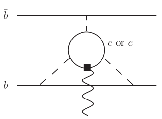
Figure 1: Leading-order diagram with a $c$-quark loop coupled to an external photon in NRQCD. Dashed lines stand for longitudinal gluons.

In the bottomonium case, if the charm-quark mass is of the same order as the typical momentum transfer in the system then it should be integrated out with that scale. Indeed it contributes to the potential hep-ph/0005066 , although in the spectrum it appears to decouple hep-ph/0108084 . The leading-order diagram with a $c$-quark loop coupled to an external photon in NRQCD is shown in Fig. 1. It is of order $\alpha_{\textrm{s}}^{3}(m_{c})\sim v^{3}$, thus beyond our accuracy.

III.3 Matching of reducible diagrams

It is useful to observe that certain classes of diagrams in NRQCD contribute just to reducible diagrams in pNRQCD, i.e. tree-level diagrams made of potentials and electromagnetic operators of lower order. Hence, they do not contribute to the matching of new operators. This happens whenever a gluonic or electromagnetic contribution can be factorized out. In the following, we will illustrate some of these cases.

• Consider static NRQCD. It describes the propagation of a static quark located in ${\bf x}_{1}$ and a static antiquark located in ${\bf x}_{2}$. We call $|n\rangle$, states that contain an arbitrary number of low-energy gluons and light quarks, but no heavy quarks. Furthermore we assume that $\psi^{\dagger}({\bf x}_{1})\chi({\bf x}_{2})|n\rangle$ is an eigenstate of the static NRQCD Hamiltonian with eigenvalue $E_{n}$. The eigenstates are normalized such that $\langle n|n\rangle=1$. In general, both $|n\rangle$ and $E_{n}$ depend on ${\bf r}$.

• The matching between NRQCD and pNRQCD follows from equating in the large time limit the time-ordered NRQCD amplitude

  $$\langle 0|\psi({\bf x}_{1})\chi^{\dagger}({\bf x}_{2})\int d^{4}z_{1}\left(\psi^{\dagger}(z_{1})O_{1}(z_{1})\psi(z_{1})+\textrm{c.c.}\right)\cdots$$

  $$\hskip 42.67912pt\times\int d^{4}z_{n}\left(\psi^{\dagger}(z_{n})O_{n}(z_{n})\psi(z_{n})+\textrm{c.c.}\right)\;\psi^{\dagger}({\bf x}^{\prime}_{1})\chi({\bf x}^{\prime}_{2})|0\rangle$$

  $$=\langle 0|\int dt_{1}\left(O_{1}(t_{1})+\textrm{c.c.}\right)\cdots\int dt_{n}\left(O_{n}(t_{n})+\textrm{c.c.}\right)$$

  $$\hskip 42.67912pt\times\theta(t_{1}-t_{2})\cdots\theta(t_{n-1}-t_{n})|0\rangle\,\delta^{3}({\bf x}_{1}-{\bf x}^{\prime}_{1})\,\delta^{3}({\bf x}_{2}-{\bf x}^{\prime}_{2}),$$

  with the corresponding pNRQCD one. The NRQCD amplitude may be identified in the large time limit with a static Wilson loop with $O_{1}$, …, $O_{n}$ and c.c. field insertions hep-ph/0002250 ; hep-ph/0009145 . The operators $O_{n}(t)$ are gluonic and electromagnetic operators in the Heisenberg representation, c.c. stands for charge conjugation (after the equality, it stands for charge conjugation and ${\bf x}_{1}\leftrightarrow{\bf x}_{2}$ exchange). The corresponding pNRQCD amplitude follows from $\psi^{\dagger}({\bf x}_{1})\chi({\bf x}_{2})|0\rangle\rightarrow S^{\dagger}({\bf r},{\bf R})|\textrm{vac}\rangle$ and $E_{0}=V_{S}^{(0)}$, where $|\textrm{vac}\rangle$ is the vacuum of pNRQCD normalized such that $\langle\textrm{vac}|\textrm{vac}\rangle=1$, see hep-ph/0002250 .

• In particular, suppose that the non-electromagnetic operator $\psi^{\dagger}O\psi+\textrm{c.c.}$ of NRQCD matches the operator $\displaystyle\int d^{3}r^{\prime\prime}\,S^{\dagger}\delta VS$ of pNRQCD, then the matching condition reads

  $$\langle 0|\int dt\,\left(O({\bf x}_{1},t)+O^{c}({\bf x}_{2},t)\right)|0\rangle\,\delta^{3}({\bf x}_{1}-{\bf x}^{\prime}_{1})\,\delta^{3}({\bf x}_{2}-{\bf x}^{\prime}_{2})$$

  $$\hskip 11.38109pt=\langle\textrm{vac}|S({\bf r},{\bf R})\,\int dt\int d^{3}R^{\prime\prime}\int d^{3}r^{\prime\prime}\,S^{\dagger}\delta VS\;\;S^{\dagger}({\bf r}^{\prime},{\bf R}^{\prime})|\textrm{vac}\rangle,$$

  where $O^{c}$ is the charge conjugated of $O$. This implies

  $$\int dt\,e^{iE_{0}t}\,\langle 0|O({\bf x}_{1})+O^{c}({\bf x}_{2})|0\rangle\,e^{-iE_{0}t}=\int dt\,e^{iV_{S}^{(0)}t}\,\delta V\,e^{-iV_{S}^{(0)}t},$$

  and eventually

  $$\langle 0|O({\bf x}_{1})+O^{c}({\bf x}_{2})|0\rangle=\delta V\,.$$ (18)

  Another example is the case of a NRQCD amplitude with insertions of two non-electromagnetic operators $\psi^{\dagger}O_{1}\psi$ and $\psi^{\dagger}O_{2}\psi$ with their charge-conjugated partners. Such an amplitude matches the pNRQCD reducible amplitude made of two insertions of $\delta V_{1}=\langle 0|O_{1}+O^{c}_{1}|0\rangle$ and $\delta V_{2}=\langle 0|O_{2}+O^{c}_{2}|0\rangle$, and the pNRQCD amplitude associated with a new potential $\delta V_{12}$,

  $$\delta V_{12}=-i\int_{0}^{\infty}dt\,\sum_{n\neq 0}\langle 0|O_{1}+O^{c}_{1}|n\rangle e^{-iE_{n}t}\langle n|O_{2}+O_{2}^{c}|0\rangle\,e^{iE_{0}t}+(1\leftrightarrow 2)\,;$$ (19)

  $n\neq 0$ intermediate state contributions that are exponentially suppressed at large times have been neglected.

• Consider now an electromagnetic operator of NRQCD, $\psi^{\dagger}O^{{\textrm{em}}}\psi+\textrm{c.c.}$, that matches the operator $\displaystyle\int d^{3}r^{\prime\prime}\,S^{\dagger}{\cal P}^{{\textrm{em}}}S$ of pNRQCD. If $O^{{\textrm{em}}}$ commutes with the gluon fields (at least to the order in the power counting we are interested in), then $O^{{\textrm{em}}}$ commutes with the static NRQCD Hamiltonian and its eigenstates (e.g. $[O^{{\textrm{em}}},|0\rangle]=0$). The argument of paragraph (iii) then implies

  $$O^{{\textrm{em}}}+O^{{\textrm{em}}\,c}={\cal P}^{{\textrm{em}}}\,.$$ (20)

• A simple extension of the previous case is the one of a NRQCD amplitude with $O_{1}$, …, $O_{n}$, $O^{{\textrm{em}}}$ field insertions under the condition that $O^{{\textrm{em}}}$ commutes with all gluonic operators $O_{1}$, …, $O_{n}$ (at the order in the power counting we are interested in). The amplitude is then proportional to

  $$O_{1}(t_{1})O_{2}(t_{2})\dots O_{n}(t_{n})O^{{\textrm{em}}}(t_{{\textrm{em}}})\Big{(}\theta(t_{{\textrm{em}}}-t_{1})\theta(t_{1}-t_{2})\dots\theta(t_{n-1}-t_{n})$$

  $$\hskip 156.49014pt+\theta(t_{1}-t_{{\textrm{em}}})\theta(t_{{\textrm{em}}}-t_{2})\dots\theta(t_{n-1}-t_{n})+\dots$$

  $$\hskip 156.49014pt+\theta(t_{1}-t_{2})\dots\theta(t_{n-1}-t_{n})\theta(t_{n}-t_{{\textrm{em}}})\Big{)}$$

  $$=O_{1}(t_{1})O_{2}(t_{2})\dots O_{n}(t_{n})\theta(t_{1}-t_{2})\dots\theta(t_{n-1}-t_{n})\;O^{{\textrm{em}}}(t_{{\textrm{em}}}),$$ (21)

  where the equality follows from the recursive use of $\theta(t_{{\textrm{em}}}-t^{\prime})\theta(t^{\prime}-t^{\prime\prime})+\theta(t^{\prime}-t_{{\textrm{em}}})\theta(t_{{\textrm{em}}}-t^{\prime\prime})=\theta(t^{\prime}-t^{\prime\prime})\theta(t_{{\textrm{em}}}-t^{\prime\prime})$. The equality implies that the amplitude reduces to the product of a pure gluonic amplitude and the electromagnetic vertex $O^{{\textrm{em}}}$. Therefore it matches the reducible diagram of pNRQCD made of some potentials (those that match the non-electromagnetic NRQCD amplitude with $O_{1}$, …, $O_{n}$ field insertions) and the electromagnetic vertex ${\cal P}^{{\textrm{em}}}$.

  

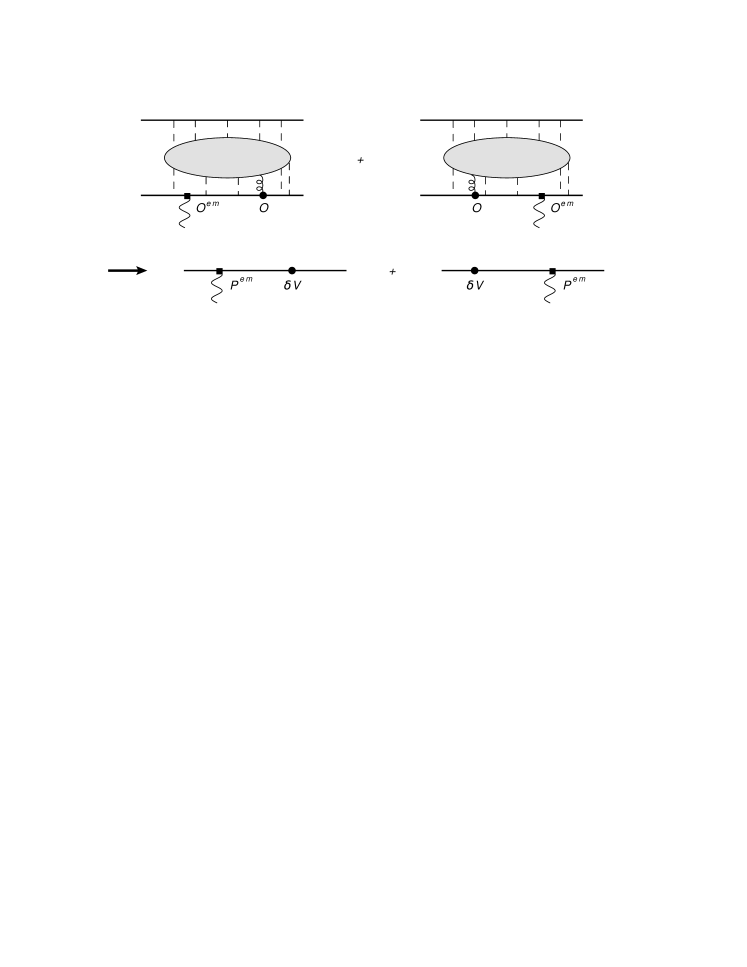
  Figure 2: Matching of the amplitude (vi): before the arrow are the NRQCD diagrams, after the arrow the pNRQCD ones. The continuous line in the pNRQCD diagrams stands for the quark-antiquark singlet propagator.

• We match now the following amplitude of NRQCD:

  $$\langle 0|\int dt_{1}\,\int dt_{2}\,\left(O({\bf x}_{1},t_{1})+\textrm{c.c}\right)\left(O^{{\textrm{em}}}({\bf x}_{1},t_{2})+\textrm{c.c}\right)\theta(t_{1}-t_{2})$$

  $$+\left(O^{{\textrm{em}}}({\bf x}_{1},t_{1})+\textrm{c.c}\right)\left(O({\bf x}_{1},t_{2})+\textrm{c.c}\right)\theta(t_{1}-t_{2})|0\rangle\,\delta^{3}({\bf x}_{1}-{\bf x}^{\prime}_{1})\,\delta^{3}({\bf x}_{2}-{\bf x}^{\prime}_{2}),$$ (22)

  under the general assumption that $O^{{\textrm{em}}}$ does not commute with $O$. By inserting a complete set of eigenstates and making use of the fact that $O^{{\textrm{em}}}$ commutes with the gluon fields, see paragraph (iv), the amplitude becomes

  $$\int dt_{1}\,\int dt_{2}\,\theta(t_{1}-t_{2})\,e^{iE_{0}t_{1}}\Bigg{\{}\langle 0|O({\bf x}_{1})+O^{c}({\bf x}_{2})|0\rangle e^{-iE_{0}(t_{1}-t_{2})}\left(O^{{\textrm{em}}}({\bf x}_{1})+O^{{\textrm{em}}\,c}({\bf x}_{2})\right)$$

  $$\hskip 28.45274pt+\left(O^{{\textrm{em}}}({\bf x}_{1})+O^{{\textrm{em}}\,c}({\bf x}_{2})\right)e^{-iE_{0}(t_{1}-t_{2})}\langle 0|O({\bf x}_{1})+O^{c}({\bf x}_{2})|0\rangle\Bigg{\}}$$

  $$\hskip 190.63338pt\times e^{-iE_{0}t_{2}}\,\delta^{3}({\bf x}_{1}-{\bf x}^{\prime}_{1})\,\delta^{3}({\bf x}_{2}-{\bf x}^{\prime}_{2})\,,$$

  which, according to (18) and (20), matches the reducible pNRQCD amplitude

  $$\int dt_{1}\,\int dt_{2}\,\theta(t_{1}-t_{2})\,e^{iV_{S}^{(0)}t_{1}}\Bigg{\{}\delta V\,e^{-iV_{S}^{(0)}(t_{1}-t_{2})}{\cal P}^{{\textrm{em}}}+{\cal P}^{{\textrm{em}}}\,e^{-iV_{S}^{(0)}(t_{1}-t_{2})}\delta V\,\Bigg{\}}$$

  $$\hskip 170.71652pt\times e^{-iV_{S}^{(0)}t_{2}}\,\delta^{3}({\bf x}_{1}-{\bf x}^{\prime}_{1})\,\delta^{3}({\bf x}_{2}-{\bf x}^{\prime}_{2})\,.$$

  Graphically this is shown in Fig. 2. Therefore an amplitude like Eq. (22) cancels in the matching against a reducible amplitude of pNRQCD.

• Finally, let us consider the case of a NRQCD amplitude with two gluonic operators $O_{1}$ and $O_{2}$ and corresponding charge-conjugated operators, and an electromagnetic operator $O^{{\textrm{em}}}$ that commutes with one of the gluonic operators, say $O_{2}$. The amplitude reads

  $$\int dt_{1}\,\int dt_{2}\,\int dt_{3}\,\theta(t_{1}-t_{2})\,\theta(t_{1}-t_{3})\,e^{iE_{0}t_{1}}$$

  $$\times\!\sum_{n}\Bigg{\{}\!\langle 0|O_{1}({\bf x}_{1})+O^{c}_{1}({\bf x}_{2})|n\rangle e^{-iE_{n}(t_{1}-t_{2})}\langle n|O_{2}({\bf x}_{1})+O^{c}_{2}({\bf x}_{2})|0\rangle\left(O^{{\textrm{em}}}({\bf x}_{1})+O^{{\textrm{em}}\,c}({\bf x}_{2})\right)\!\!\Bigg{\}}$$

  $$\hskip 190.63345pt\times e^{-iE_{0}t_{2}}\,\delta^{3}({\bf x}_{1}-{\bf x}^{\prime}_{1})\,\delta^{3}({\bf x}_{2}-{\bf x}^{\prime}_{2})$$

  $$+\int dt_{1}\,\int dt_{2}\,\int dt_{3}\,\theta(t_{1}-t_{2})\,\theta(t_{3}-t_{1})\,e^{iE_{0}t_{1}}$$

  $$\times\!\sum_{n}\Bigg{\{}\!\left(O^{{\textrm{em}}}({\bf x}_{1})+O^{{\textrm{em}}\,c}({\bf x}_{2})\right)\langle 0|O_{1}({\bf x}_{1})+O^{c}_{1}({\bf x}_{2})|n\rangle e^{-iE_{n}(t_{1}-t_{2})}\langle n|O_{2}({\bf x}_{1})+O^{c}_{2}({\bf x}_{2})|0\rangle\!\!\Bigg{\}}$$

  $$\hskip 190.63345pt\times e^{-iE_{0}t_{2}}\,\delta^{3}({\bf x}_{1}-{\bf x}^{\prime}_{1})\,\delta^{3}({\bf x}_{2}-{\bf x}^{\prime}_{2})$$

  $$+\,(1\leftrightarrow 2)\,.$$ (23)

  The $n=0$ component of the amplitude matches the reducible pNRQCD diagrams made of insertions of the potentials $\delta V_{1}$, $\delta V_{2}$ and of the electromagnetic vertex ${\cal P}^{{\textrm{em}}}$. The sum of the $n\neq 0$ components matches

  $$\int dt_{1}\,\int dt_{2}\,\theta(t_{1}-t_{2})\,e^{iV_{S}^{(0)}t_{1}}\Bigg{\{}i\delta V_{12}\,e^{-iV_{S}^{(0)}(t_{1}-t_{2})}{\cal P}^{{\textrm{em}}}+{\cal P}^{{\textrm{em}}}\,e^{-iV_{S}^{(0)}(t_{1}-t_{2})}i\delta V_{12}\,\Bigg{\}}$$

  $$\hskip 170.71652pt\times e^{-iV_{S}^{(0)}t_{2}}\,\delta^{3}({\bf x}_{1}-{\bf x}^{\prime}_{1})\,\delta^{3}({\bf x}_{2}-{\bf x}^{\prime}_{2})\,.$$

  Therefore, also this kind of amplitude does not induce new operators in pNRQCD.

III.4 Matching at $\mathcal{O}(1/m^{0})$

Amplitudes that contribute to the $\mathcal{O}(1/m^{0})$ matching of $\mathcal{L}_{\gamma\textrm{pNRQCD}}$ may contain the NRQCD operators (see Eq. (2))

$$-\psi^{\dagger}ee_{Q}A_{0}^{{\textrm{em}}}\psi,\quad-\psi^{\dagger}gA_{0}\psi\,,$$ (24)

and the corresponding c.c. ones. Although they just contain one electromagnetic operator, they may contain an arbitrary number of longitudinal gluons for they are not suppressed by any power of $1/m$. The electromagnetic field $A_{0}^{{\textrm{em}}}$ commutes with the gluon fields. Therefore it satisfies the condition of Sec. III.3, paragraph (iv), and the matching condition is given by Eq. (20). It tells that electromagnetic operators of order $1/m^{0}$ do not get QCD corrections. Hence all $\mathcal{O}(1/m^{0})$ Wilson coefficients of $\mathcal{L}_{\gamma\textrm{pNRQCD}}$ are fixed at their ${\cal O}(\alpha_{\textrm{s}}^{0})$ value:

$$V^{r\cdot E}=V^{(r\nabla)^{2}r\cdot E}=1\,.$$ (25)

For weakly-coupled quarkonia, also the quark-antiquark color-octet sector is relevant. In this case, the matching is performed by considering NRQCD amplitudes between initial and final states that match the color octet state in pNRQCD hep-ph/9907240 . Since the electromagnetic field commutes also with these states, the result of the matching to all orders is

$$V_{O}^{r\cdot E}=1\,.$$ (26)

Finally, we observe that, while our argument fixes $V^{r\cdot E}$ to all orders, the same argument does not apply to the Wilson coefficient $V_{A}$ of the chromoelectric dipole operator in Eq. (7). The reason is that the field $A_{0}$ does not commute with the gluon fields.

III.5 Matching at $\mathcal{O}(1/m)$

Amplitudes that contribute to the $\mathcal{O}(1/m)$ matching of $\mathcal{L}_{\gamma\textrm{pNRQCD}}$ contain, besides an arbitrary number of operators of order $1/m^{0}$, one of the NRQCD operators of order $1/m$ (see Eq. (2)):

$$\psi^{\dagger}\frac{{\bf D}^{2}}{2m}\psi,\quad\frac{c_{F}}{2m}\psi^{\dagger}\boldsymbol{\sigma}\cdot g{\bf B}\,\psi,\quad\frac{c_{F}^{{\textrm{em}}}}{2m}\psi^{\dagger}\boldsymbol{\sigma}\cdot ee_{Q}{\bf B}^{{\textrm{em}}}\psi,$$ (27)

and the corresponding c.c. ones. We call the first operator the kinetic energy operator, the second one the chromomagnetic dipole operator and the third one the magnetic dipole operator. The $\mathcal{O}(1/m)$ amplitudes fall in one of the following categories.

1. The photon is coupled to the magnetic dipole operator. This kind of diagrams matches spin-dependent operators and may contribute to $V^{(r\nabla)\sigma\cdot B}$. Using the same argument as for the $1/m^{0}$ matching, the amplitude factorizes. Therefore, it holds to all orders that

$$V^{(r\nabla)\sigma\cdot B}=c_{F}^{{\textrm{em}}}\,,$$ (28)

and no other operator is generated.

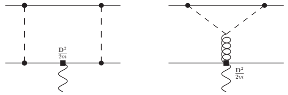
Figure 3: Examples of diagrams at order $1/m$, where the electromagnetic coupling is contained in a covariant derivative.

2. The photon is coupled to the kinetic energy operator (see e.g. Fig. 3). This kind of diagrams matches only operators with magnetic fields, hence they may contribute to $V^{\nabla\cdot(r\times B)}$ and $V^{\nabla_{r}\cdot(r\times(r\nabla)B)}$. Since the electromagnetic coupling is embedded in a covariant derivative operator,

$$\psi^{\dagger}(\boldsymbol{\nabla}-iee_{Q}{\bf A}^{{\textrm{em}}})\psi+\textrm{c.c.}\,,$$ (29)

this implies that diagrams involving one kinetic energy operator match pNRQCD operators of the form

$$\int d^{3}r\;S^{\prime\,\dagger}\,\left(\left\{\frac{{\delta V_{a}}}{m},\left(\mbox{\boldmath$\nabla$}_{x_{1}}-iee_{Q}{\bf A}^{{\textrm{em}}}({\bf x}_{1},t)\right)^{2}\right\}+\textrm{c.c.}\right)S^{\prime}$$

$$+\int d^{3}r\;S^{\prime\,\dagger}\,\left(\left\{\frac{{\delta V_{b}}}{m}{\bf r}\cdot,i\left(\mbox{\boldmath$\nabla$}_{x_{1}}-iee_{Q}{\bf A}^{{\textrm{em}}}({\bf x}_{1},t)\right)\right\}+\textrm{c.c.}\right)S^{\prime}\,.$$ (30)

After the field redefinition (13) and having multipole expanded the electromagnetic fields up to include order $r^{2}$ contributions, the pNRQCD operators may be rewritten as

$$\int d^{3}r\;S^{\dagger}\,\left\{\frac{{\delta V_{a}}}{m},\frac{\mbox{\boldmath$\nabla$}^{2}}{2}+2\mbox{\boldmath$\nabla$}_{r}^{2}+2\left\{i\mbox{\boldmath$\nabla$},\frac{{\bf r}\times ee_{Q}{\bf B}^{{\textrm{em}}}}{4}\right\}+2\left\{i\mbox{\boldmath$\nabla$}_{r},\frac{{\bf r}\times[({\bf r}\cdot\mbox{\boldmath$\nabla$})ee_{Q}{\bf B}^{{\textrm{em}}}]}{12}\right\}\right\}S$$

$$+\int d^{3}r\;S^{\dagger}\,\left\{\frac{{\delta V_{b}}}{m}{\bf r}\cdot,2i\mbox{\boldmath$\nabla$}_{r}\right\}S\,.$$ (31)

Switching off the electromagnetic interaction, this expression should match Eq. (6), which fixes $\delta V_{a}=1/4$ and $\delta V_{b}=0$ to all orders in perturbation theory. The fact that the kinetic energy in pNRQCD is protected against quantum corrections is a direct consequence of Poincaré invariance hep-ph/0306107 . We conclude, therefore, that

$$V^{\nabla\cdot(r\times B)}=V^{\nabla_{r}\cdot(r\times(r\nabla)B)}=1$$ (32)

holds to all orders in perturbation theory.

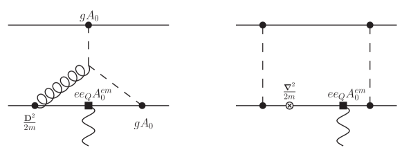
Figure 4: Examples of diagrams at order $1/m$ with an external longitudinal photon.

3. The photon is longitudinal and coupled to the heavy quark/antiquark lines. Such diagrams match only operators with electric fields. If we consider diagrams with one insertion of a chromomagnetic dipole operator or a kinetic energy operator (for the latter see Fig. 4), then such diagrams may possibly contribute at order $1/m$ to operators that vanish at ${\cal O}(\alpha_{\textrm{s}}^{0})$, for instance,

$$\int d^{3}r\;\frac{1}{mr}S^{\dagger}{\bf r}\cdot ee_{Q}{\bf E}^{{\textrm{em}}}S\,.$$ (33)

In both cases, the argument developed in Sec. III.3, paragraph (vi), applies, for $A_{0}^{{\textrm{em}}}$ commutes with gluons. Hence, all such diagrams cancel in the matching against reducible pNRQCD diagrams, and an operator like the one written above does not show up even at higher orders in the coupling constant.

III.6 Matching at $\mathcal{O}(1/m^{2})$

Diagrams that contribute to the matching at order $1/m^{2}$ contain, besides an arbitrary number of operators of order $1/m^{0}$, either two operators of order $1/m$ or one of the following operators of order $1/m^{2}$:

$$\frac{c_{S}}{8m^{2}}\boldsymbol{\sigma}\cdot[i{\bf D}\times,g{\bf E}],\quad\frac{c_{S}^{{\textrm{em}}}}{8m^{2}}\boldsymbol{\sigma}\cdot[i{\bf D}\times,ee_{Q}{\bf E}^{{\textrm{em}}}],\quad\frac{c_{D}}{8m^{2}}[{\bf D}\cdot,g{\bf E}],\quad\frac{c_{D}^{{\textrm{em}}}}{8m^{2}}ee_{Q}(\mbox{\boldmath$\nabla$}\cdot{\bf E}^{{\textrm{em}}})\,,$$

which we call the (chromo)electric spin-orbit operator and the (chromo)electric Darwin operator respectively. Since many different diagrams can contribute, it is convenient to distinguish between spin-dependent and spin-independent amplitudes. It is always implicitly assumed that diagrams may contain an arbitrary number of $1/m^{0}$ gluonic vertices.

III.6.1 Spin-dependent diagrams

First, we consider the matching of spin-dependent operators.

1. We consider diagrams made of two chromomagnetic dipole operators and a longitudinal photon. Since the photon commutes with the chromomagnetic dipole operators, the result of Sec. III.3, paragraph (v), applies: these diagrams do not contribute to the matching of new operators.

2. Diagrams that contain one magnetic dipole operator and a chromomagnetic dipole one are of the type discussed in Sec. III.3, paragraph (vi). Hence they do not contribute to the matching of new operators. Moreover, in hep-ph/0512369 , it has been pointed out that this kind of amplitudes, proportional to the expectation value of a chromomagnetic field, vanishes for parity.

3. The situation is similar for diagrams that contain one magnetic dipole operator and a kinetic energy one. Since the magnetic dipole operator commutes with the gluons, we are in the situation of Sec. III.3, paragraph (vi), and this type of diagrams does not contribute to the matching of new operators.

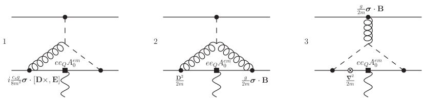
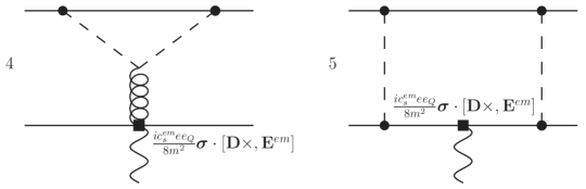
Figure 5: Some diagrams that contribute to spin-dependent operators of order $1/m^{2}$ containing an electric field.

4. Also diagrams that contain one chromoelectric spin-orbit operator and one longitudinal photon (see e.g. diagram 1 in Fig. 5) fall under the situation discussed in Sec. III.3, paragraph (vi), and do not contribute to the matching of new operators.

5. We consider now diagrams made with one chromomagnetic dipole operator, one kinetic energy operator and a longitudinal photon (see e.g. diagrams 2 and 3 in Fig. 5). Since the longitudinal photon commutes with the chromomagnetic dipole operator, the argument of Sec. III.3, paragraph (vii), applies and therefore such diagrams do not contribute to the matching of new operators in pNRQCD.

6. Diagrams that contain one electric spin-orbit operator (see e.g. diagrams 4 and 5 in Fig. 5) contribute to operators that are at least $v^{2}$ suppressed with respect to the leading electric dipole operator of pNRQCD. These operators depend on spin and on an electric field. For time inversion invariance, they must also depend on the quarkonium momentum. Hence, only the derivative part of the covariant derivative of the electric spin-orbit operator contributes and only if it does not act on the gluon fields. Since $\displaystyle\frac{c_{S}^{{\textrm{em}}}}{8m^{2}}\boldsymbol{\sigma}\cdot[-i{\mbox{\boldmath$\nabla$}}\times,ee_{Q}{\bf E}^{{\textrm{em}}}]$ effectively acts as an operator that commutes with the gluons, we are in the situation discussed in Sec. III.3, paragraph (iv), that led to the matching condition (20). In our case and at leading order in the multipole expansion, the matching condition becomes

$$V^{\sigma\cdot(E\times\nabla_{r})}=c_{S}^{{\textrm{em}}}\,,$$ (34)

which is exact. Operators that come from higher-orders in the multipole expansion do not need to be considered here because they are beyond our accuracy (although the matching fixes also the Wilson coefficients of those operators to all orders). Operators that are possible for symmetry arguments alone, like for instance

$$\frac{1}{m^{2}r^{2}}[\mathrm{S}^{\dagger},\mbox{\boldmath$\sigma$}^{i}]\left\{({\bf r}\times i\mbox{\boldmath$\nabla$}_{r})^{i},{\bf r}\cdot ee_{Q}{\bf E}^{{\textrm{em}}}\right\}\mathrm{S},$$

cannot be generated at any order in the strong-coupling constant and, therefore, may be set to zero in pNRQCD. Finally, we observe that the observation made in hep-ph/0002250 that $\langle 0|{\bf D}_{x_{1}}|0\rangle=\mbox{\boldmath$\nabla$}_{x_{1}}$ and $\langle 0|{\bf D}_{x_{2}}|0\rangle=\mbox{\boldmath$\nabla$}_{x_{2}}$ would lead to the same result.

7. Diagrams containing either one chromomagnetic operator and a kinetic energy operator coupled to an external photon or one chromoelectric spin-orbit operator with the electromagnetic field encoded in the covariant derivative have been calculated to all orders in hep-ph/0512369 with an argument similar to the one used in Sec. III.5, paragraph 2. They contribute to the Wilson coefficient of one single operator,

$$\frac{1}{4m^{2}}\;\frac{1}{r^{3}}\;\left\{{\rm S}^{\dagger},\mbox{\boldmath$\sigma$}\cdot\left[{\bf r}\times\left({\bf r}\times ee_{Q}{\bf B}^{{\textrm{em}}}\right)\right]\right\}{\rm S}\,,$$ (35)

which, however, is relevant only for M1 transitions and not for E1 ones, since it does not change the parity of the quarkonium state.

III.6.2 Spin-independent diagrams

Now we consider the matching of spin-independent operators.

1. Diagrams with one insertion of an electric Darwin operator do not contribute beyond ${\cal O}(\alpha_{\textrm{s}}^{0})$ to the matching, for the electric Darwin operator commutes with gluons and the conclusion of Sec. III.3, paragraph (iv), applies. These diagrams match into the electric Darwin operator of pNRQCD. Such an operator has not been displayed in Eq. (II.2), because it does not contribute to E1 transitions.

2. Diagrams that contain one chromoelectric Darwin operator and a longitudinal photon are of the type discussed in Sec. III.3, paragraph (v). The electromagnetic interaction factorizes and the contribution cancels in the matching.

3. We consider diagrams containing two kinetic energy operators. The (transverse) electromagnetic field is embedded in one of the covariant derivatives. These diagrams match spin-independent operators of pNRQCD with one magnetic field. Because of the pNRQCD symmetry under charge conjugation and ${\bf x}_{1}\leftrightarrow{\bf x}_{2}$ exchange, the allowed spin-independent operators with one magnetic field must contain an odd number of ${\bf r}$ or $\boldsymbol{\nabla}_{r}$. Moreover, because of parity invariance, at least one center of mass derivative has to be present too. However, such operators are too much suppressed to be relevant for E1 transitions at relative order $v^{2}$, an example being the operator

$$\frac{1}{m^{2}r}{\rm S}^{\dagger}\{i\boldsymbol{\nabla}\cdot,{\bf r}\times ee_{Q}{\bf B}^{{\textrm{em}}}\}{\rm S}\,,$$

which is of relative order $v^{3}$ with respect to the leading electric dipole operator.

Figure 6: Some diagrams contributing to the matching of spin-independent operators of order $1/m^{2}$.

4. Finally, we consider diagrams containing two kinetic energy operators and an external longitudinal photon, see Fig. 6. We observe that $A_{0}^{{\textrm{em}}}({\bf x}_{1})+A_{0}^{{\textrm{em}}\,c}({\bf x}_{2})={\bf r}\cdot\mbox{\boldmath$\nabla$}A_{0}^{{\textrm{em}}}+{\cal O}(r^{2})$. Hence, these diagrams contribute to operators that are at least $1/m^{2}\times(mv)^{2}\sim v^{2}$ suppressed with respect to the leading electric dipole operator of pNRQCD; operators generated by higher orders in the multipole expansion are beyond our accuracy. Let us consider now the kinetic energy operators. If one of the derivatives acts on the longitudinal photon then the diagrams contribute to operators that are at least $v^{3}$ suppressed with respect to the leading electric dipole operator of pNRQCD. Operators of relative order $v^{3}$ are beyond our accuracy. If one of the derivatives acts on the factor ${\bf r}$ in ${\bf r}\cdot\mbox{\boldmath$\nabla$}A_{0}^{{\textrm{em}}}$ then the other derivatives do not. As a consequence, the electromagnetic operator ${\bf r}\cdot\mbox{\boldmath$\nabla$}A_{0}^{{\textrm{em}}}$ commutes at relative order $v^{2}$ with at least one of the kinetic energy operators and we are in the situation described in Sec. III.3, paragraph (vii). We conclude that in pNRQCD these diagrams cancel against iterations of lower-order potentials and electromagnetic vertices and do not contribute to any new operator. In particular, possible operators allowed by the symmetries of pNRQCD, like, for instance,

$$\frac{1}{m^{2}r^{2}}{\rm S}^{\dagger}{\bf r}\cdot ee_{Q}{\bf E}^{{\textrm{em}}}{\rm S}\,,\qquad\frac{1}{m^{2}}{\rm S}^{\dagger}\left\{\mbox{\boldmath$\nabla$}_{r}^{2},{\bf r}\cdot ee_{Q}{\bf E}^{{\textrm{em}}}\right\}{\rm S}\,,$$

cannot be generated at any order in the strong-coupling constant.

III.7 Concluding remarks

In this section, we have matched non-perturbatively all operators of pNRQCD relevant to describe E1 transitions at relative order $v^{2}$. It turns out that the situation for E1 transitions is different from the one for M1 transitions first discussed in hep-ph/0512369 .

For E1 transitions no $\mathcal{O}(1/m^{3})$ operator is relevant at relative order $v^{2}$, as it is shown in Eq. (II.2). In particular, we can neglect the matching of NRQCD diagrams with three kinetic energy operator insertions or with one insertion of the operator ${\bf D}^{4}/(8m^{3})$.

For M1 transitions between strongly-coupled states, corrections of relative order $v^{2}$ require the non-perturbative matching of $1/m^{3}$ operators. At this order one can perform an exact matching for all but one relevant operator (see appendix). This is the operator

$$\frac{1}{m^{3}r^{2}}\,V^{\frac{\sigma\cdot B}{m^{3}}}\,\left\{{\rm S}^{\dagger},\mbox{\boldmath$\sigma$}\cdot ee_{Q}{\bf B}^{{\textrm{em}}}\right\}{\rm S}\,,$$ (36)

whose Wilson coefficient, $V^{\frac{\sigma\cdot B}{m^{3}}}$, can possibly get QCD corrections at the momentum-transfer scale. These are encoded in the expectation value of some suitable Wilson loop, whose explicit expression is at present unknown.

IV E1 transitions

After having derived the relevant pNRQCD Lagrangian, we will now proceed in the calculation of the electric dipole transition rates, starting from the non-relativistic limit. This will be used to fix the notation and discuss the wave functions. We will follow closely hep-ph/0512369 .

IV.1 Quarkonium states

We consider radiative transitions, $H\rightarrow H^{\prime}\,\gamma$, between a quarkonium $H$ and a quarkonium $H^{\prime}$. A quarkonium state $\lvert H({\bf P},\lambda)\rangle$ is an eigenstate of the pNRQCD Hamiltonian with the quantum numbers of a quarkonium $H$ with polarization $\lambda$. We normalize it in the non-relativistic way, i.e.

$$\langle H({\bf P}^{\prime},\lambda^{\prime})\lvert H({\bf P},\lambda)\rangle=(2\pi)^{3}\delta^{3}({\bf P}-{\bf P}^{\prime})\delta_{\lambda\lambda^{\prime}}\,.$$ (37)

The leading-order quarkonium state is defined as

$$\lvert H({\bf P},\lambda)\rangle^{(0)}= \int d^{3}R\int d^{3}r\,e^{i\bf P\cdot R}\textrm{Tr}\left\{\phi^{(0)}_{H(\lambda)}({\bf r})\textrm{S}^{\dagger}({\bf r},{\bf R})|\textrm{vac}\rangle\right\}\,,$$ (38)

which is also an eigenstate of the total spin, the orbital angular momentum and the center of mass momentum ${\bf P}$ of the quark-antiquark pair. The wave function $\phi^{(0)}_{H(\lambda)}({\bf r})$ is an eigenfunction of the leading pNRQCD singlet Hamiltonian $h^{(0)}_{S}$, i.e. a solution of the Schrödinger equation

$$h^{(0)}_{S}\phi^{(0)}_{H(\lambda)}\equiv\left(-\frac{{\boldsymbol{\nabla}_{r}}^{2}}{m}+V_{S}^{(0)}\right)\phi^{(0)}_{H(\lambda)}=E^{(0)}_{H}\phi^{(0)}_{H(\lambda)}\,.$$ (39)

The eigenvalue $E^{(0)}_{H}$ is the leading-order binding energy.

The wave functions have the following angular structures for $L=0$ hep-ph/0512369

$$\phi^{(0)}_{n^{1}S_{0}}({\bf r}) = \sqrt{\frac{1}{8\pi}}\,R_{n0}(r)\,,$$ (40)

$$\phi^{(0)}_{n^{3}S_{1}(\lambda)}({\bf r}) = \sqrt{\frac{1}{8\pi}}\,R_{n0}(r)\,\boldsymbol{\sigma}\cdot{\bf e}_{n^{3}S_{1}}(\lambda)\,,$$ (41)

for $L=1$

$$\phi^{(0)}_{n^{1}P_{1}(\lambda)}({\bf r}) = \sqrt{\frac{3}{8\pi}}\,R_{n1}(r)\,{\bf e}_{n^{1}P_{1}}(\lambda)\cdot\hat{\bf r}\,,$$ (42)

$$\phi^{(0)}_{n^{3}P_{0}}({\bf r}) = \sqrt{\frac{1}{8\pi}}\,R_{n1}(r)\boldsymbol{\sigma}\cdot\hat{\bf r}\,,$$ (43)

$$\phi^{(0)}_{n^{3}P_{1}(\lambda)}({\bf r}) = \sqrt{\frac{3}{16\pi}}\,R_{n1}(r)\,\boldsymbol{\sigma}\cdot(\hat{\bf r}\times{\bf e}_{n^{3}P_{1}}(\lambda))\,,$$ (44)

$$\phi^{(0)}_{n^{3}P_{2}(\lambda)}({\bf r}) = \sqrt{\frac{3}{8\pi}}\,R_{n1}(r)\,\boldsymbol{\sigma}^{i}h^{ij}_{n^{3}P_{2}}(\lambda)\hat{\bf r}^{j}\,,$$ (45)

and for $L=2$ arXiv:1007.4541 ; Piotr

$$\phi^{(0)}_{n^{1}D_{2}(\lambda)}({\bf r}) = \sqrt{\frac{15}{16\pi}}\,R_{n2}(r)\,\hat{\bf r}^{i}h^{ij}_{n^{1}D_{2}}(\lambda)\hat{\bf r}^{j}\,,$$ (46)

$$\phi^{(0)}_{n^{3}D_{1}(\lambda)}({\bf r}) = \sqrt{\frac{1}{16\pi}}\,R_{n2}(r)\,\left[3({\bf e}_{n^{3}D_{1}}(\lambda)\cdot\hat{\bf r})(\boldsymbol{\sigma}\cdot\hat{\bf r})-\boldsymbol{\sigma}\cdot{\bf e}_{n^{3}D_{1}}(\lambda)\right]\,,$$ (47)

$$\phi^{(0)}_{n^{3}D_{2}(\lambda)}({\bf r}) = \sqrt{\frac{5}{8\pi}}\,R_{n2}(r)\,\hat{\bf r}^{i}h^{ij}_{n^{3}D_{2}}(\lambda)({\hat{\bf r}\times\boldsymbol{\sigma}})^{j}\,,$$ (48)

$$\phi^{(0)}_{n^{3}D_{3}(\lambda)}({\bf r}) = \sqrt{\frac{15}{16\pi}}\,R_{n2}(r)\,\hat{\bf r}^{i}\hat{\bf r}^{j}H^{ijk}_{n^{3}D_{3}}(\lambda)\boldsymbol{\sigma}^{k}\,.$$ (49)

The vectors ${\bf e}_{n^{2S+1}L_{J}}(\lambda)$ denote orthonormal polarization vectors of the quarkonium state. The tensors $h^{ij}_{n^{2S+1}L_{J}}(\lambda)$ and $H^{ijk}_{n^{2S+1}L_{J}}(\lambda)$ are completely symmetric, traceless (the tensor $H^{ijk}$ has vanishing partial traces, i.e. $H^{iik}_{n^{2S+1}L_{J}}=0$) and normalized as

$$h^{ij\,\ast}_{n^{2S+1}L_{J}}(\lambda)h^{ij}_{n^{2S+1}L_{J}}(\lambda^{\prime})=\delta_{\lambda\lambda^{\prime}}=H^{ijk\,\ast}_{n^{2S+1}L_{J}}(\lambda)H^{ijk}_{n^{2S+1}L_{J}}(\lambda^{\prime})\,.$$ (50)

Whereas the quarkonium state is normalized in the non-relativistic fashion (37), the one photon state, $\lvert\gamma({\bf k},\sigma)\rangle$, is normalized in the usual Lorentz-invariant way

$$\langle\gamma({\bf k},\sigma)\lvert\gamma({\bf k}^{\prime},\sigma^{\prime})\rangle=2k(2\pi)^{3}\delta^{3}({\bf k}-{\bf k}^{\prime})\delta_{\sigma\sigma^{\prime}}\,.$$ (51)

This implies that external electric or magnetic fields project on a one photon state as

$$\langle\gamma({\bf k},\sigma)\lvert{\bf E}^{{\textrm{em}}}({\bf R})\lvert\textrm{vac}\rangle = -ik{\boldsymbol{\epsilon}}^{\ast}(\sigma)e^{-i{\bf k}\cdot{\bf R}}\,,$$ (52)

$$\langle\gamma({\bf k},\sigma)|{\bf B}^{{\textrm{em}}}({\bf R})|\textrm{vac}\rangle = -i\,{\bf k}\times\mbox{\boldmath$\epsilon$}^{*}(\sigma)\,e^{-i{\bf k}\cdot{\bf R}}\,,$$ (53)

where ${\boldsymbol{\epsilon}}(\sigma)$ is the photon polarization vector (the dependence of ${\boldsymbol{\epsilon}}(\sigma)$ on ${\bf k}$ is understood). The photon transversality requires ${\boldsymbol{\epsilon}}(\sigma)\cdot{\bf k}=0$.

Finally, the quarkonium and photon polarizations satisfy the relations

$$\sum_{\lambda}{\bf e}^{i\,\ast}_{n^{2S+1}L_{J}}(\lambda){\bf e}^{j}_{n^{2S+1}L_{J}}(\lambda) = \delta^{ij}\,,$$ (54)

$$\sum_{\lambda}h^{ij\,\ast}_{n^{2S+1}L_{J}}(\lambda)h^{kl}_{n^{2S+1}L_{J}}(\lambda) = \frac{1}{2}(\delta^{ik}\delta^{jl}+\delta^{il}\delta^{jk})-\frac{1}{3}\delta^{ij}\delta^{kl}\,,$$ (55)

$$\sum_{\lambda}H^{ijk\,\ast}_{n^{2S+1}L_{J}}(\lambda)H^{lmn}_{n^{2S+1}L_{J}}(\lambda) = \frac{1}{(3!)^{2}}\left(\delta^{il}\delta^{jm}\delta^{kn}-\frac{3}{5}\delta^{ij}\delta^{kl}\delta^{mn}\right.$$ (56)

$$+\,\hbox{permutations of the indices $i,j,k$ and $l,m,n$}\Big{)}\,,$$

$$\sum_{\sigma}{\boldsymbol{\epsilon}}^{i}(\sigma){\boldsymbol{\epsilon}}^{j\,\ast}(\sigma) = \delta^{ij}-\hat{\bf k}^{i}\hat{\bf k}^{j}\,.$$ (57)

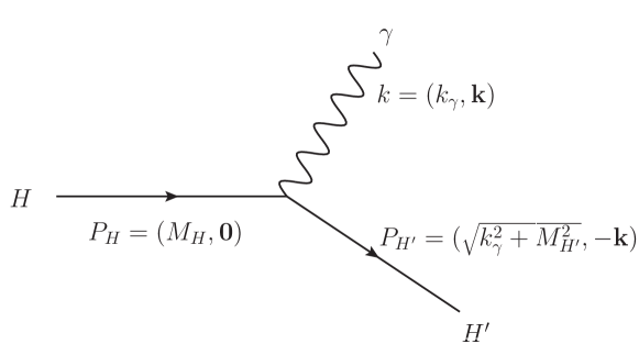
Figure 7: Kinematics of the transition $H\rightarrow H^{\prime}\,\gamma$ in the center of mass frame.

IV.2 Transition amplitudes and rates

In the rest frame of the initial quarkonium, see Fig. 7, the transition amplitude from a quarkonium $H$ with polarization $\lambda$ to a quarkonium $H^{\prime}$ with momentum ${\bf P}^{\prime}$ and polarization $\lambda^{\prime}$, and a photon with energy

$$k_{\gamma}=\lvert{\bf k}\rvert=\frac{M_{H}^{2}-M_{H^{\prime}}^{2}}{2M_{H}}=(M_{H}-M_{H}^{\prime})+\,\mathcal{O}\left(\frac{k_{\gamma}^{2}}{M_{H}}\right),$$ (58)

and polarization $\sigma$ is given by

$${\cal A}\left[H({\bf 0},\lambda)\to H^{\prime}(-{\bf k},\lambda^{\prime})\gamma({\bf k},\sigma)\right](2\pi)^{3}\delta^{3}({\bf P}^{\prime}+{\bf k}) =$$ (59)

$$-\langle H^{\prime}({\bf P}^{\prime},\lambda^{\prime})\gamma({\bf k},\sigma)\lvert\int d^{3}R\,\mathcal{L}_{\gamma\textrm{pNRQCD}}\,\lvert H({\bf 0},\lambda)\rangle\,.$$

The corresponding transition width reads

$$\Gamma_{H\rightarrow H^{\prime}\,\gamma}= \,\int\frac{d^{3}P^{\prime}}{(2\pi)^{3}}\frac{d^{3}k}{(2\pi)^{3}}\frac{1}{2k}\,(2\pi)^{4}\delta^{4}(P_{H}-k-P^{\prime})\,\frac{1}{N_{\lambda}}\sum_{\lambda\lambda^{\prime}\sigma}\lvert\mathcal{A}_{H\rightarrow H^{\prime}\,\gamma}\rvert^{2}$$

$$= \,\frac{1}{8\pi^{2}}\left(1-\frac{k_{\gamma}}{M_{H}}\right)\int_{0}^{\infty}\!\!dk\,k\int d\Omega({\bf\hat{k}})\,\delta(k-k_{\gamma})\frac{1}{N_{\lambda}}\sum_{\lambda\lambda^{\prime}\sigma}\lvert\mathcal{A}_{H\rightarrow H^{\prime}\,\gamma}\rvert^{2}\,,$$ (60)

where the initial state is averaged over the polarizations, whose number is $N_{\lambda}$, and $\mathcal{A}_{H\rightarrow H^{\prime}\,\gamma}$ is a short-hand notation for ${\cal A}\left[H({\bf 0},\lambda)\to H^{\prime}(-{\bf k},\lambda^{\prime})\gamma({\bf k},\sigma)\right]$.

IV.3 The non-relativistic limit

The leading operator responsible for E1 transitions in pNRQCD is the electric dipole operator

$$\mathcal{L}_{E1}=\int d^{3}r\,\mathrm{Tr}\,\left\{{\rm S}^{\dagger}{\bf r}\cdot ee_{Q}{\bf E}^{{\textrm{em}}}{\rm S}\right\}\,.$$ (61)

From Eqs. (38), (52), (59) and the equal-time commutation rules for singlet fields (spin indices are written down explicitly)

$$\left[{S}^{\dagger}_{ij}({\bf r},{\bf R},t),{S}_{kl}({\bf r}^{\prime},{\bf R}^{\prime},t)\right]=\delta_{il}\delta_{jk}\delta^{3}({\bf r}-{\bf r}^{\prime})\delta^{3}({\bf R}-{\bf R}^{\prime}),$$ (62)

it follows that the leading amplitudes for the E1 transitions $n^{3}P_{J}\rightarrow n^{\prime\,3}S_{1}\,\gamma$ and $n^{1}P_{1}\rightarrow n^{\prime\,1}S_{0}\,\gamma$ read

$$\mathcal{A}^{(0)}_{n^{3}P_{0}\rightarrow n^{\prime\,3}S_{1}\,\gamma}=\frac{iee_{Q}k}{3}\,I_{3}(n1\rightarrow n^{\prime}0)\,{\boldsymbol{\epsilon}}^{\ast}(\sigma)\cdot{\bf e}_{n^{\prime\,3}S_{1}}(\lambda^{\prime})\,,$$ (63)

$$\mathcal{A}^{(0)}_{n^{3}P_{1}\rightarrow n^{\prime\,3}S_{1}\,\gamma}=\frac{iee_{Q}k}{\sqrt{6}}\,I_{3}(n1\rightarrow n^{\prime}0)\,{\boldsymbol{\epsilon}}^{\ast}(\sigma)\cdot({\bf e}_{n^{3}P_{1}}(\lambda)\times{\bf e}_{n^{\prime\,3}S_{1}}(\lambda^{\prime}))\,,$$ (64)

$$\mathcal{A}^{(0)}_{n^{3}P_{2}\rightarrow n^{\prime\,3}S_{1}\,\gamma}=\frac{iee_{Q}k}{\sqrt{3}}\,I_{3}(n1\rightarrow n^{\prime}0)\,{\bf e}_{n^{\prime\,3}S_{1}}^{i}(\lambda^{\prime})h^{ij}_{n^{3}P_{2}}(\lambda){\boldsymbol{\epsilon}}^{\ast\,j}(\sigma)\,,$$ (65)

$$\mathcal{A}^{(0)}_{n^{1}P_{1}\rightarrow n^{\prime\,1}S_{0}\,\gamma}=\frac{iee_{Q}k}{\sqrt{3}}\,I_{3}(n1\rightarrow n^{\prime}0)\,{\boldsymbol{\epsilon}}^{\ast}(\sigma)\cdot{\bf e}_{n^{1}P_{1}}(\lambda)\,,$$ (66)

where we have defined

$$I_{N}(nL\rightarrow n^{\prime}L^{\prime}) = \int_{0}^{\infty}dr\,r^{N}\,R_{n^{\prime}L^{\prime}}(r)\,R_{nL}(r)\,,$$ (67)

$$I^{\prime}_{N}(nL\rightarrow n^{\prime}L^{\prime}) = \int_{0}^{\infty}dr\,r^{N}\,R_{n^{\prime}L^{\prime}}(r)\,\frac{d}{dr}R_{nL}(r)\,.$$ (68)

The second definition is for further use. We also give the amplitudes for $n^{3}D_{1}\rightarrow n^{\prime\,3}P_{J}\,\gamma$:

$$\mathcal{A}^{(0)}_{n^{3}D_{1}\rightarrow n^{\prime\,3}P_{0}\,\gamma}=\frac{iee_{Q}k\sqrt{2}}{3}\,I_{3}(n2\rightarrow n^{\prime}1)\,{\boldsymbol{\epsilon}}^{\ast}(\sigma)\cdot{\bf e}_{n^{3}D_{1}}(\lambda)\,,$$ (69)

$$\mathcal{A}^{(0)}_{n^{3}D_{1}\rightarrow n^{\prime\,3}P_{1}\,\gamma}=\frac{iee_{Q}k}{2\sqrt{3}}\,I_{3}(n2\rightarrow n^{\prime}1)\,{\boldsymbol{\epsilon}}^{\ast}(\sigma)\cdot({\bf e}_{n^{3}D_{1}}(\lambda)\times{\bf e}_{n^{\prime\,3}P_{1}}(\lambda^{\prime}))\,,$$ (70)

$$\mathcal{A}^{(0)}_{n^{3}D_{1}\rightarrow n^{\prime\,3}P_{2}\,\gamma}=\frac{iee_{Q}k}{5\sqrt{6}}\,I_{3}(n2\rightarrow n^{\prime}1)\,{\bf e}_{n^{3}D_{1}}^{i}(\lambda)h^{ij}_{n^{\prime\,3}P_{2}}(\lambda^{\prime}){\boldsymbol{\epsilon}}^{\ast\,j}(\sigma)\,.$$ (71)

From (IV.2) and the relations (54-57), it follows that the non-relativistic decay rates are

$$\Gamma^{(0)}_{n^{3}P_{J}\rightarrow n^{\prime\,3}S_{1}\,\gamma} = \Gamma^{(0)}_{nn^{\prime}}\left(1-\frac{k_{\gamma}}{M_{n^{3}P_{J}}}\right)\,,$$ (72)

$$\Gamma^{(0)}_{n^{1}P_{1}\rightarrow n^{\prime\,1}S_{0}\,\gamma} = \Gamma^{(0)}_{nn^{\prime}}\left(1-\frac{k_{\gamma}}{M_{n^{1}P_{1}}}\right)\,,$$ (73)

with

$$\Gamma^{(0)}_{nn^{\prime}}\equiv\frac{4}{9}\,\alpha e_{Q}^{2}k_{\gamma}^{3}[I_{3}(n1\rightarrow n^{\prime}0)]^{2}\,\sim\frac{k_{\gamma}^{3}}{m^{2}v^{2}}\,.$$ (74)

E1 transition rates are of order ${k_{\gamma}^{3}}/{(m^{2}v^{2})}$, which means that they happen $1/v^{2}$ more frequently than allowed M1 transitions at the same photon energy. The terms proportional to $k_{\gamma}/M_{n^{3}P_{J}}\sim k_{\gamma}/M_{n^{1}P_{1}}\sim mv^{2}/(2m)$ are suppressed by $v^{2}$ and can therefore be neglected at leading order. They contribute and have to be accounted for at relative order $v^{2}$, which we will compute in the next section. We note that at leading order the transition rate is independent of the initial total angular momentum $J$. The reverse transitions depend instead on the final total angular momentum:

$$\Gamma^{(0)}_{n^{3}S_{1}\rightarrow n^{\prime\,3}P_{J}\,\gamma}= \,\frac{2J+1}{3}\Gamma^{(0)}_{nn^{\prime}}\left(1-\frac{k_{\gamma}}{M_{n^{3}S_{1}}}\right)\,,$$ (75)

$$\Gamma^{(0)}_{n^{1}S_{0}\rightarrow n^{\prime\,1}P_{1}\,\gamma}= \,3\Gamma^{(0)}_{nn^{\prime}}\left(1-\frac{k_{\gamma}}{M_{n^{1}S_{0}}}\right)\,.$$ (76)

These results agree, neglecting $k_{\gamma}/m$ corrections, with the general non-relativistic formula Eichten:1978tg

$$\Gamma^{(0)}_{n^{2S+1}L_{J}\rightarrow n^{\prime 2S+1}L^{\prime}_{J^{\prime}}\,\gamma}=\frac{4}{3}\,\alpha e_{Q}^{2}\,k_{\gamma}^{3}\,[I_{3}(nL\rightarrow n^{\prime}L^{\prime})]^{2}\,(2J^{\prime}+1)\,\textrm{max}(L,L^{\prime})\,\left\{\begin{array}[]{ccc}J&1&J^{\prime}\\ L^{\prime}&S&L\end{array}\right\}^{2},$$ (77)

where the last term in the brackets denotes a Wigner 6-j coefficient.

V Relativistic corrections to E1 transitions

One of the main advantages of using pNRQCD is that it accounts for the corrections to the decay amplitudes in a systematic fashion. We will split the analysis into a part that accounts for the electromagnetic interaction terms in the pNRQCD Lagrangian suppressed by $\mathcal{O}(v^{2})$ with respect to the leading electric dipole operator (61), and a part that accounts for $v^{2}$ corrections to the quarkonium state. We will concentrate on the decay $n^{3}P_{J}\rightarrow n^{\prime\,3}S_{1}\,\gamma$ to compare with the result in PRINT-84-0308 . The extension to other processes like $n^{1}P_{1}\rightarrow n^{\prime\,1}S_{0}\,\gamma$, $n^{3}S_{1}\rightarrow n^{\prime\,3}P_{J}\,\gamma$ and $n^{1}S_{0}\rightarrow n^{\prime\,1}P_{1}\,\gamma$ is straightforward. Final results for all these radiative transitions will be given in Sec. VI. For a non-vanishing leading-order transition amplitude $\mathcal{A}^{(0)}_{n^{2S+1}L_{J}(\lambda)\rightarrow n^{\prime\,2S+1}{L^{\prime}}_{J^{\prime}}(\lambda^{\prime})\,\gamma}$, we define

$$\bar{\mathcal{A}}\equiv\frac{\mathcal{A}}{\mathcal{A}^{(0)}}\,,\qquad\bar{{\Gamma}}\equiv\frac{\Gamma}{\Gamma^{(0)}}\,.$$ (78)

V.1 Corrections induced by E1 operators of relative order $v^{2}$

At subleading order in the decay rate, i.e. at order $k_{\gamma}^{3}/m^{2}$, all the interaction terms displayed in the Lagrangian (II.2) beyond the leading electric dipole operator contribute.

• The correction induced by the operator $S^{\dagger}{\bf r}\cdot[({\bf r}\cdot{\boldsymbol{\nabla}})^{2}ee_{Q}{\bf E}^{{\textrm{em}}}]S/24$ is

  $$\bar{\mathcal{A}}^{(1)}_{n^{3}P_{J}\rightarrow n^{\prime\,3}S_{1}\,\gamma}=-\frac{k^{2}}{120}\frac{I_{5}(n1\rightarrow n^{\prime}0)}{I_{3}(n1\rightarrow n^{\prime}0)}\,.$$ (79)

• The correction induced by the operator $iS^{\dagger}\{{\boldsymbol{\nabla}}\cdot,{\bf r}\times ee_{Q}{\bf B}^{{\textrm{em}}}\}S/(4m)$ is

  $$\bar{\mathcal{A}}^{\textrm{(2)}}_{n^{3}P_{J}\rightarrow n^{\prime\,3}S_{1}\,\gamma}=\frac{k}{4m}\,.$$ (80)

• The operator $iS^{\dagger}\{{\boldsymbol{\nabla}}_{r}\cdot,{\bf r}\times[({{\bf r}\cdot{\boldsymbol{\nabla}}})ee_{Q}{\bf B}^{{\textrm{em}}}]\}S/(12m)$ corrects the leading-order amplitude by an amount

  $$\bar{\mathcal{A}}^{\textrm{(3)}}_{n^{3}P_{J}\rightarrow n^{\prime\,3}S_{1}\,\gamma}=-\frac{k}{12m}\,.$$ (81)

• The spin-dependent operator $c_{F}^{{\textrm{em}}}[S^{\dagger},{\boldsymbol{\sigma}}]\cdot[({\bf r}\cdot{\boldsymbol{\nabla}})ee_{Q}{\bf B}^{{\textrm{em}}}]S/(4m)$ contributes with

  $$\bar{\mathcal{A}}^{(4)}_{n^{3}P_{0}\rightarrow n^{\prime\,3}S_{1}\,\gamma}=\frac{kc_{F}^{{\textrm{em}}}}{2m}\,,$$ (82)

  $$\bar{\mathcal{A}}^{(4)}_{n^{3}P_{1}\rightarrow n^{\prime\,3}S_{1}\,\gamma}=\frac{kc_{F}^{{\textrm{em}}}}{2m}\frac{(\hat{\bf k}\cdot{\bf e}_{n^{\prime\,3}S_{1}}){\boldsymbol{\epsilon}}^{\ast}\cdot(\hat{\bf k}\times{\bf e}_{n^{3}P_{1}})}{{\boldsymbol{\epsilon}}^{\ast}\cdot({\bf e}_{n^{\prime\,3}S_{1}}\times{\bf e}_{n^{3}P_{1}})}\,,$$ (83)

  $$\bar{\mathcal{A}}^{(4)}_{n^{3}P_{2}\rightarrow n^{\prime\,3}S_{1}\,\gamma}=\frac{kc_{F}^{{\textrm{em}}}}{2m}\frac{\left[({\boldsymbol{\epsilon}}^{\ast}\cdot{\bf e}_{n^{\prime\,3}S_{1}})\hat{\bf k}^{i}-(\hat{\bf k}\cdot{\bf e}_{n^{\prime\,3}S_{1}}){\boldsymbol{\epsilon}}^{\ast\,i}\right]h^{ij}_{n^{3}P_{2}}\hat{\bf k}^{j}}{{\boldsymbol{\epsilon}}^{\ast\,i}h^{ij}_{n^{3}P_{2}}{\bf e}^{j}_{n^{\prime\,3}S_{1}}}\,,$$ (84)

  where the quarkonium and photon polarization numbers are not explicitly shown. Using Eqs. (54)-(57) the corresponding decay rates yield

  $$\bar{{\Gamma}}^{(4)}_{n^{3}P_{J}\rightarrow n^{\prime\,3}S_{1}\,\gamma}=-\frac{k_{\gamma}c_{F}^{{\textrm{em}}}}{2m}\left[\frac{J(J+1)}{2}-2\right]\,.$$ (85)

• Finally, the contribution of the operator $-ic_{S}^{{\textrm{em}}}[S^{\dagger},{\boldsymbol{\sigma}}]\cdot(ee_{Q}{\bf E}^{{\textrm{em}}}\times{\boldsymbol{\nabla}}_{r})S/(4m^{2})$ is

  $$\bar{\mathcal{A}}^{(5)}_{n^{3}P_{J}\rightarrow n^{\prime\,3}S_{1}\,\gamma}=\frac{c_{S}^{{\textrm{em}}}}{2m^{2}}\left[\frac{J(J+1)}{2}-2\right]\frac{I_{2}^{\prime}(n1\rightarrow n^{\prime}0)+2I_{1}(n1\rightarrow n^{\prime}0)}{I_{3}(n1\rightarrow n^{\prime}0)}\,.$$ (86)

V.2 Quarkonium state corrections of relative order $v^{2}$

The quarkonium state (38) is not an eigenstate of the complete Hamiltonian of pNRQCD. The eigenstate may be constructed from (38) by systematically adding higher-order corrections, which are perturbative in the relative velocity $v$. Corrections may come from higher-order potentials ($1/m$ and $1/m^{2}$ terms) and from higher Fock states, which account for the coupling of the quark-antiquark singlet state to other low-energy degrees of freedom. We have to include such corrections at relative order $v^{2}$, both in the initial and in the final quarkonium states, in order to achieve a precision of relative order $v^{2}$ in the E1 transition rates.

V.2.1 Corrections due to higher-order potentials

The first-order correction to the quarkonium state (38) induced by a correction $\delta h_{S}$ to the Hamiltonian $h_{S}^{(0)}$ is given by

$$\lvert H({\bf P},\lambda)\rangle^{(1)} = \int\frac{d^{3}P^{\prime}}{(2\pi)^{3}}\,\sum_{H^{\prime}\neq H,\lambda^{\prime}}\frac{|H^{\prime}({\bf P}^{\prime},\lambda^{\prime})\rangle^{(0)}\;{}^{(0)}\langle H^{\prime}({\bf P}^{\prime},\lambda^{\prime})|}{E_{H}^{(0)}-E_{H^{\prime}}^{(0)}}$$ (87)

$$\hskip 85.35826pt\times\int d^{3}R\int d^{3}r\,\textrm{Tr}\left\{\textrm{S}^{\dagger}\delta h_{S}(r)\textrm{S}\right\}|H({\bf P},\lambda)\rangle^{(0)}\,.$$

We assume that, in order to account for corrections of relative order $v^{2}$, we need to include in $\delta h_{S}$ all the $1/m$ and $1/m^{2}$ potentials and, at order $1/m^{3}$, the first relativistic correction to the kinetic energy. Such a counting, which holds for weakly-coupled quarkonia, appears to be generally consistent with heavy quarkonium spectroscopy hep-ph/9407339 , and it is indeed the most widely used. It should be remarked, however, that in the case of strongly-coupled quarkonia it is not the most conservative one hep-ph/0009145 .

In the assumed power counting, at relative order $v^{2}$, $\delta h_{S}$ has the form

$$\delta h_{S}(r)=-\frac{{\bf p}^{4}}{4m^{3}}+\delta V_{S}(r)\,,$$ (88)

where ${\bf p}=-i\boldsymbol{\nabla}_{r}$. $\delta V_{S}$ is organized in powers of $1/m$,

$$\delta V_{S}(r)=\frac{V^{(1)}(r)}{m}+\frac{V^{(2)}_{\rm SI}(r)}{m^{2}}+\frac{V^{(2)}_{\rm SD}(r)}{m^{2}}\,,$$ (89)

where, at order $1/m^{2}$, we have distinguished between spin independent (SI) and spin dependent (SD) terms hep-ph/0410047 ,

$$V^{(2)}_{\rm SI}(r)= V^{(2)}_{r}(r)+\frac{1}{2}\{V^{(2)}_{p^{2}}(r),{\bf p}^{2}\}+\frac{V^{(2)}_{L^{2}}(r)}{r^{2}}{\bf L}^{2}\,,$$ (90)

$$V^{(2)}_{\rm SD}(r)= V^{(2)}_{LS}(r){\bf L}\cdot{\bf S}+V^{(2)}_{S^{2}}(r){\bf S}^{2}+V^{(2)}_{S_{12}}(r){\bf S}_{12}(\hat{\bf r})\,,$$ (91)

with ${\bf S}={\bf S}_{1}+{\bf S}_{2}=({\boldsymbol{\sigma}}_{1}+{\boldsymbol{\sigma}}_{2})/2$, ${\bf L}={\bf r}\times{\bf p}$ and ${\bf S}_{12}(\hat{\bf r})=3(\hat{\bf r}\cdot\boldsymbol{\sigma}_{1})(\hat{\bf r}\cdot\boldsymbol{\sigma}_{2})-\boldsymbol{\sigma}_{1}\cdot\boldsymbol{\sigma}_{2}$. Terms involving the center of mass momentum, which is $-{\bf k}_{\gamma}$ for the quarkonium in the final state, are suppressed by an extra $v$ and have been neglected. In the weak-coupling case, the above potentials read at leading (non-vanishing) order in perturbation theory (see e.g. hep-ph/9910238 )

$$V^{(1)}(r)=-\frac{C_{F}N_{c}\alpha_{\textrm{s}}^{2}}{2r^{2}}\,,\quad V^{(2)}_{r}(r)=\pi C_{F}\alpha_{\textrm{s}}\delta^{3}({\bf r})\,,\quad V^{(2)}_{p^{2}}(r)=-\frac{C_{F}\alpha_{\textrm{s}}}{r}\,,\quad V^{(2)}_{L^{2}}(r)=\frac{C_{F}\alpha_{\textrm{s}}}{2r}\,,$$

$$V^{(2)}_{LS}(r)=\frac{3C_{F}\alpha_{\textrm{s}}}{2r^{3}}\,,\quad V^{(2)}_{S^{2}}(r)=\frac{4\pi C_{F}\alpha_{\textrm{s}}}{3}\delta^{3}({\bf r})\,,\quad V^{(2)}_{S_{12}}(r)=\frac{C_{F}\alpha_{\textrm{s}}}{4r^{3}}\,.$$ (92)

In the strong-coupling case, the potentials are non-perturbative and can be expressed in terms of Wilson loops to be eventually evaluated on the lattice hep-ph/0009145 .

There are, however, some observations that can be made without relying on any specific form of the potential, but just on its general structure (89)-(91). Let us consider the radiative transition $n^{3}P_{J}\rightarrow n^{\prime\,3}S_{1}\,\gamma$. Initial state corrections due to $\delta h_{S}$ read

$$\mathcal{A}^{\textrm{i}}_{n^{3}P_{J}\rightarrow n^{\prime\,3}S_{1}\,\gamma} = -{}^{(0)}\langle n^{\prime\,3}S_{1}\,\gamma\lvert\int d^{3}R\;\mathcal{L}_{E1}\,\lvert n^{3}P_{J}\rangle^{(1)}$$ (93)

$$= \sum_{m\neq n}\frac{{}^{(0)}\langle m^{3}P_{J}\lvert\delta h_{S}(r)\lvert n^{3}P_{J}\rangle^{(0)}}{E^{(0)}_{n1}-E^{(0)}_{m1}}\,\mathcal{A}^{(0)}_{m^{3}P_{J}\rightarrow n^{\prime\,3}S_{1}\,\gamma}\,,$$

where $E^{(0)}_{nL}$ is the leading-order binding energy of a quarkonium with principal quantum number $n$ and orbital angular momentum $L$. Final state corrections read

$$\mathcal{A}^{\textrm{f}}_{n^{3}P_{J}\rightarrow n^{\prime\,3}S_{1}\,\gamma} = -{}^{(1)}\langle n^{\prime\,3}S_{1}\gamma\lvert\int d^{3}R\;\mathcal{L}_{E1}\,\lvert n^{3}P_{J}\rangle^{(0)}$$ (94)

$$= \sum_{m\neq n^{\prime}}\frac{{}^{(0)}\langle n^{\prime\,3}S_{1}\lvert\delta h_{S}(r)\lvert m^{3}S_{1}\rangle^{(0)}}{E^{(0)}_{n^{\prime}0}-E^{(0)}_{m0}}\,\mathcal{A}^{(0)}_{n^{3}P_{J}\rightarrow m^{3}S_{1}\,\gamma}$$

$$+\sum_{m,J^{\prime}}\frac{{}^{(0)}\langle n^{\prime\,3}S_{1}\lvert\delta h_{S}(r)\lvert m^{3}D_{J^{\prime}}\rangle^{(0)}}{E^{(0)}_{n^{\prime}0}-E^{(0)}_{m2}}\,\mathcal{A}^{(0)}_{n^{3}P_{J}\rightarrow m^{3}D_{J^{\prime}}\,\gamma}\,.$$

In both expressions, a sum over the intermediate state polarizations is understood. We have made use of the selection rule for the electric dipole matrix element and of the fact that the potentials (89)-(91) do not change the total angular momentum of the state, which follows from BS

$$\langle n^{2S+1}L_{J}|\,V^{(2)}_{LS}(r)\,{\bf L}\cdot{\bf S}\,|n^{\prime\,2S^{\prime}+1}L^{\prime}_{J^{\prime}}\rangle = \delta_{LL^{\prime}}\delta_{JJ^{\prime}}\delta_{SS^{\prime}}\frac{J(J+1)-L(L+1)-S(S+1)}{2}$$ (95)

$$\hskip 76.82234pt\times\langle n^{2S+1}L_{J}|\,V^{(2)}_{LS}(r)\,|n^{\prime\,2S+1}L_{J}\rangle,$$

$$\langle n^{2S+1}L_{J}|\,V^{(2)}_{S^{2}}(r)\,{\bf S}^{2}\,|n^{\prime\,2S^{\prime}+1}L^{\prime}_{J^{\prime}}\rangle = \delta_{LL^{\prime}}\delta_{JJ^{\prime}}\delta_{SS^{\prime}}\;S(S+1)\;\langle n^{2S+1}L_{J}|\,V^{(2)}_{S^{2}}(r)\,|n^{\prime\,2S+1}L_{J}\rangle,$$

$$\langle n^{2S+1}L_{J}|\,V^{(2)}_{S_{12}}(r)\,{\bf S}_{12}(\hat{\bf r})\,|n^{\prime\,2S^{\prime}+1}L_{J^{\prime}}\rangle = \delta_{JJ^{\prime}}\delta_{SS^{\prime}}\langle{\bf S}_{12}\rangle_{LJS}\langle n^{2S+1}L_{J}|\,V^{(2)}_{S_{12}}(r)\,|n^{\prime\,2S+1}L_{J}\rangle,$$ (97)

where $\langle{\bf S}_{12}\rangle_{101}=-4$, $\langle{\bf S}_{12}\rangle_{111}=2$, $\langle{\bf S}_{12}\rangle_{121}=-2/5$, $\langle{\bf S}_{12}\rangle_{0JS}=0$ and $\langle{\bf S}_{12}\rangle_{LJ0}=0$. For the final state correction, we have assumed a completely non-degenerate spectrum. To complete the spin structure of the wave-function corrections, we need to compute ${}^{(0)}\langle n^{3}S_{1}\lvert\,V^{(2)}_{S_{12}}(r)\,\lvert m^{3}D_{J}\rangle^{(0)}$. It turns out that this matrix element does not vanish only for $J=1$ and in this case

$${}^{(0)}\langle n^{3}S_{1}\lvert\,V^{(2)}_{S_{12}}(r)\,\lvert m^{3}D_{1}\rangle^{(0)}=-2\sqrt{2}\,{\bf e}_{m^{3}D_{1}}\cdot{\bf e}_{n^{3}S_{1}}\int_{0}^{\infty}dr\,r^{2}\,R_{n0}(r)R_{m2}(r)\,V^{(2)}_{S_{12}}(r)\,.$$ (98)

Summing over the intermediate state polarizations allows to factorize the leading order amplitude. For instance, in the case of the contribution of the spin-tensor potential $V^{(2)}_{S_{12}}(r){\bf S}_{12}(\hat{\bf r})/m^{2}$ to the initial and final states, we obtain

$$\bar{\mathcal{A}}_{n^{3}P_{J}\rightarrow n^{\prime\,3}S_{1}\,\gamma}^{\textrm{i}}\Big{|}_{S_{12}}= \frac{1}{m^{2}}\sum_{m\neq n}\frac{\displaystyle\int_{0}^{\infty}dr\,r^{2}\,R_{m1}(r)R_{n1}(r)\,V^{(2)}_{S_{12}}(r)}{E^{(0)}_{n1}-E^{(0)}_{m1}}\frac{I_{3}(m1\rightarrow n^{\prime}0)}{I_{3}(n1\rightarrow n^{\prime}0)}\langle{\bf S}_{12}\rangle_{1J1}\,,$$ (99)

$$\bar{\mathcal{A}}_{n^{3}P_{J}\rightarrow n^{\prime\,3}S_{1}\,\gamma}^{\textrm{f}}\Big{|}_{S_{12}}= \frac{1}{m^{2}}\sum_{m}\frac{\displaystyle\int_{0}^{\infty}dr\,r^{2}\,R_{n^{\prime}0}(r)R_{m2}(r)\,V^{(2)}_{S_{12}}(r)}{E^{(0)}_{n^{\prime}0}-E^{(0)}_{m2}}\frac{I_{3}(n1\rightarrow m2)}{I_{3}(n1\rightarrow n^{\prime}0)}\langle{\bf S}_{12}\rangle_{1J1}\,.$$ (100)

Analogous results hold for the other potentials. The complete correction to the transition width coming from higher-order potentials is of the form

$$\bar{{\Gamma}}^{\textrm{h.o. potentials}}_{n^{3}P_{J}\rightarrow n^{\prime\,3}S_{1}\,\gamma}=R^{S=1}_{nn^{\prime}}(J)\,,$$ (101)

$$\bar{{\Gamma}}^{\textrm{h.o. potentials}}_{n^{1}P_{1}\rightarrow n^{\prime\,1}S_{0}\,\gamma}=R^{S=0}_{nn^{\prime}}\,,$$ (102)

where the general spin structure of $R^{S=1}_{nn^{\prime}}(J)$ is $R^{S=1}_{nn^{\prime}}(J)=A_{nn^{\prime}}+2B_{nn^{\prime}}+C_{nn^{\prime}}J(J+1)+D_{nn^{\prime}}\langle{\bf S}_{12}\rangle_{1J1}$ ($B_{nn^{\prime}}$ is the correction coming from the spin-spin potential) and the general spin structure of $R^{S=0}_{nn^{\prime}}$ is $R^{S=0}_{nn^{\prime}}=A_{nn^{\prime}}+2C_{nn^{\prime}}$. The specific values of the coefficients $A_{nn^{\prime}}$, $B_{nn^{\prime}}$, $C_{nn^{\prime}}$ and $D_{nn^{\prime}}$, which involve expressions similar to the ones displayed in Eqs. (99) and (100), depend on the form of the potentials and will not be discussed further in this work.

V.2.2 Corrections due to higher Fock states

The quarkonium initial and final states may also get corrections from the coupling of the heavy quark-antiquark pair to other low-energy degrees of freedom. We call these corrections higher Fock state corrections.

For strongly-coupled quarkonia, we argued that we can neglect couplings with other low-energy degrees of freedom, see Sec. II.2. In this case, we do not have new corrections coming from higher Fock states.

For weakly-coupled quarkonia, we have to account for the coupling with low-energy gluons, see Eq. (7). A higher Fock state contributing at order $v^{2}$ is made of a gluon and a heavy quark-antiquark pair in a color-octet configuration. Moreover, photons may couple to a quark-antiquark octet state through (10). Again we consider the radiative transition $n^{3}P_{J}\rightarrow n^{\prime\,3}S_{1}\,\gamma$, whose relevant diagrams at relative order $v^{2}$ are shown in Fig. 8.

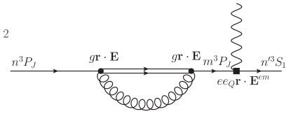
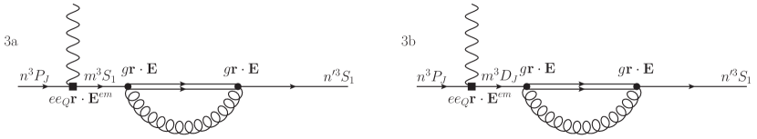
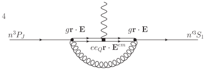
Figure 8: Color-octet contributions to the E1 transition $n^{3}P_{J}\rightarrow n^{\prime\,3}S_{1}\,\gamma$ for weakly-coupled states. The double line stands for an intermediate octet state.

The first two diagrams correspond to the normalization of the initial and final states, $(\delta Z_{n^{3}P_{J}}+\delta Z_{n^{\prime\,3}S_{1}})/2$. They can be calculated from the self energy of the state, first derived in hep-ph/9907240 , which is given for a generic quarkonium $H$ by

$$\delta E_{H(\lambda)} = -\frac{i}{6}\int_{0}^{\infty}\!\!dt\;\langle\textrm{vac}\lvert gE^{a\,i}({\bf R},t)\phi(t,0)^{\textrm{adj}}_{ab}gE^{b\,i}({\bf R},0)\lvert\textrm{vac}\rangle$$ (103)

$$\hskip 113.81102pt\times{}^{(0)}\langle H({\bf 0},\lambda)\lvert r^{j}e^{-i(h_{O}^{(0)}-E_{H}^{(0)})t}r^{j}\lvert H({\bf 0},\lambda)\rangle^{(0)}\,,$$

where the Wilson line in the adjoint representation is

$$\phi(t,0)^{\textrm{adj}}_{ab}=\left(e^{\displaystyle-ig\int_{0}^{t}dt^{\prime}A_{0}({\bf R},t^{\prime})^{\textrm{adj}}}\right)_{ab}\,,$$ (104)

and $h_{O}^{(0)}\equiv-\mbox{\boldmath$\nabla$}^{2}_{r}/m+V_{O}^{(0)}$. Deriving the self energy with respect to the energy provides the state normalization

$$\delta Z_{H(\lambda)}=\frac{\partial\delta E_{H(\lambda)}}{\partial E^{(0)}_{H}} = \frac{1}{6}\int_{0}^{\infty}\!\!dt\,t\;\langle\textrm{vac}\lvert gE^{a\,i}({\bf R},t)\phi(t,0)^{\textrm{adj}}_{ab}gE^{b\,i}({\bf R},0)\lvert\textrm{vac}\rangle$$ (105)

$$\hskip 56.9055pt\times{}^{(0)}\langle H({\bf 0},\lambda)\lvert r^{j}e^{-i(h_{O}^{(0)}-E_{H}^{(0)})t}r^{j}\lvert H({\bf 0},\lambda)\rangle^{(0)}\,.$$

Thus, the contribution from the state normalizations to the amplitude reads

$$\mathcal{A}^{\textrm{Fig.~{}\ref{color-octet}},\;1}_{n^{3}P_{J}\rightarrow n^{\prime\,3}S_{1}\,\gamma} = \frac{\mathcal{A}^{(0)}_{n^{3}P_{J}\rightarrow n^{\prime\,3}S_{1}\,\gamma}}{12}\int_{0}^{\infty}dt\,t\;\langle\textrm{vac}\lvert gE^{a\,i}({\bf R},t)\phi(t,0)^{\textrm{adj}}_{ab}gE^{b\,i}({\bf R},0)\lvert\textrm{vac}\rangle$$ (106)

$$\times\left[{}^{(0)}\langle n^{3}P_{J}\lvert r^{j}e^{-i(h_{O}^{(0)}-E_{n1}^{(0)})t}r^{j}\lvert n^{3}P_{J}\rangle^{(0)}+{}^{(0)}\langle n^{\prime\,3}S_{1}\lvert r^{j}e^{-i(h_{O}^{(0)}-E_{n^{\prime}0}^{(0)})t}r^{j}\lvert n^{\prime\,3}S_{1}\rangle^{(0)}\right].$$

Diagram 2, the initial state correction, yields

$$\mathcal{A}^{\textrm{Fig.~{}\ref{color-octet}},\;2}_{n^{3}P_{J}\rightarrow n^{\prime\,3}S_{1}\,\gamma} = -\frac{i}{6}\sum_{m\neq n}\frac{\mathcal{A}^{(0)}_{m^{3}P_{J}\rightarrow n^{\prime\,3}S_{1}\,\gamma}}{E_{n1}^{(0)}-E_{m1}^{(0)}}\int_{0}^{\infty}dt\,\langle\textrm{vac}\lvert gE^{a\,i}({\bf R},t)\phi(t,0)^{\textrm{adj}}_{ab}gE^{b\,i}({\bf R},0)\lvert\textrm{vac}\rangle$$ (107)

$$\times{}^{(0)}\langle m^{3}P_{J}\lvert r^{j}e^{-i(h_{O}^{(0)}-E_{n1}^{(0)})t}r^{j}\lvert n^{3}P_{J}\rangle^{(0)}\,,$$

while diagrams 3a and 3b, the final state corrections, yield

$$\mathcal{A}^{\textrm{Fig.~{}\ref{color-octet}},\;3\textrm{a}}_{n^{3}P_{J}\rightarrow n^{\prime\,3}S_{1}\,\gamma} = -\frac{i}{6}\sum_{m\neq n^{\prime}}\frac{\mathcal{A}^{(0)}_{n^{3}P_{J}\rightarrow m^{3}S_{1}\,\gamma}}{E_{n^{\prime}0}^{(0)}-E_{m0}^{(0)}}\int_{0}^{\infty}dt\,\langle\textrm{vac}\lvert gE^{a\,i}({\bf R},t)\phi(t,0)^{\textrm{adj}}_{ab}gE^{b\,i}({\bf R},0)\lvert\textrm{vac}\rangle$$ (108)

$$\times{}^{(0)}\langle n^{\prime\,3}S_{1}\lvert r^{j}e^{-i(h_{O}^{(0)}-E_{n^{\prime}0}^{(0)})t}r^{j}\lvert m^{3}S_{1}\rangle^{(0)}\,,$$

$$\mathcal{A}^{\textrm{Fig.~{}\ref{color-octet}},\;3\textrm{b}}_{n^{3}P_{J}\rightarrow n^{\prime\,3}S_{1}\,\gamma} = 0\,.$$ (109)

$\mathcal{A}^{\textrm{Fig.~{}\ref{color-octet}},\;3\textrm{b}}$ vanishes, since $r^{j}\,\textrm{e}^{-i(h_{O}^{(0)}-E_{n^{\prime}0}^{(0)})t}\,r^{j}$ is a scalar that cannot change the angular momentum. The contribution from the last diagram, where the photon is coupled to an intermediate octet state, reads

$$\mathcal{A}^{\textrm{Fig.~{}\ref{color-octet}},\;4}_{n^{3}P_{J}\rightarrow n^{\prime\,3}S_{1}\,\gamma} = -\frac{i}{6}\int_{0}^{\infty}dt\int_{0}^{t}dt^{\prime}\,\langle\textrm{vac}\lvert gE^{a\,i}({\bf R},t)\phi(t,0)^{\textrm{adj}}_{ab}gE^{b\,i}({\bf R},0)\lvert\textrm{vac}\rangle$$ (110)

$$\times{}^{(0)}\langle n^{\prime\,3}S_{1}\lvert r^{j}e^{-i(h_{O}^{(0)}-E_{n^{\prime}0}^{(0)})(t-t^{\prime})}{ee_{Q}k{\boldsymbol{\epsilon}}^{\ast}(\sigma)\cdot\bf r}e^{-i(h_{O}^{(0)}-E_{n1}^{(0)})t^{\prime}}r^{j}\lvert n^{3}P_{J}\rangle^{(0)}.$$

According to the power counting of Sec. II.2, all amplitudes (106)-(110) contribute to relative order $1/(mv)^{2}\times\Lambda_{\textrm{QCD}}^{2}\sim v^{2}$ or $1/(mv)^{2}\times\Lambda_{\textrm{QCD}}^{3}\times 1/(mv^{2})\sim v^{2}$, where the factor $1/(mv)^{2}$ comes from the two $r^{j}$ and we have assumed the chromoelectric correlator to scale like $\Lambda_{\textrm{QCD}}^{4}\sim(mv^{2})^{4}$.

It is noteworthy that, in contrast to M1 transitions hep-ph/0512369 , weak-coupling non-perturbative contributions do not cancel for E1 transitions. This is due to the fact that the leading electric dipole operator does not commute with the kinetic energy. Hence, even in the weak coupling, E1 transitions are affected at order $v^{2}$ by non-perturbative contributions. These are encoded in the chromoelectric correlator $\langle\textrm{vac}\lvert gE^{a\,i}({\bf R},t)\phi(t,0)^{\textrm{adj}}_{ab}gE^{b\,i}({\bf R},0)\lvert\textrm{vac}\rangle$. For $E\gg\Lambda_{\textrm{QCD}}$, the correlator reduces to the gluon condensate, which factorizes; however, this scale hierarchy is unlikely to be of relevance for E1 transitions.

VI Results and comparison with the literature

Now we can summarize our results and compare them with PRINT-84-0308 . The results are obtained by summing up all corrections calculated in the previous section, which include contributions coming from E1 operators of relative order $v^{2}$, and initial and final state corrections. The complete decay rates $n^{3}P_{J}\rightarrow n^{\prime\,3}S_{1}\gamma$ and $n^{1}P_{J}\rightarrow n^{\prime\,1}S_{0}\gamma$, this last one obtained by leaving out spin-dependent contributions from the former expression, read to order $k_{\gamma}^{3}/m^{2}$

$$\Gamma_{n^{3}P_{J}\rightarrow n^{\prime\,3}S_{1}\,\gamma} = \Gamma^{(0)}_{nn^{\prime}}\left[1+R_{nn^{\prime}}^{S=1}(J)-\frac{k_{\gamma}}{6m}-\frac{k_{\gamma}^{2}}{60}\frac{I_{5}(n1\rightarrow n^{\prime}0)}{I_{3}(n1\rightarrow n^{\prime}0)}\right.$$

$$\left.+\left(\frac{J(J+1)}{2}-2\right)\left(-(1+\kappa_{Q}^{{\textrm{em}}})\frac{k_{\gamma}}{2m}+\frac{1}{m^{2}}(1+2\kappa_{Q}^{{\textrm{em}}})\frac{I_{2}^{\prime}(n1\rightarrow n^{\prime}0)+2I_{1}(n1\rightarrow n^{\prime}0)}{I_{3}(n1\rightarrow n^{\prime}0)}\right)\right],$$

$$\Gamma_{n^{1}P_{1}\rightarrow n^{\prime\,1}S_{0}\,\gamma} = \Gamma^{(0)}_{nn^{\prime}}\left[1+R_{nn^{\prime}}^{S=0}-\frac{k_{\gamma}}{6m}-\frac{k_{\gamma}^{2}}{60}\frac{I_{5}(n1\rightarrow n^{\prime}0)}{I_{3}(n1\rightarrow n^{\prime}0)}\right].$$ (112)

$R_{nn^{\prime}}^{S=1}(J)$ and $R_{nn^{\prime}}^{S=0}$ are the initial and final state corrections; they include corrections coming from higher-order potentials, see Sec. V.2.1, and, in the case of weakly-coupled quarkonia, the color-octet contributions computed in Eqs. (106)-(110). We have kept terms proportional to the anomalous magnetic moment, $\kappa_{Q}^{{\textrm{em}}}$, for the sake of the following comparison, though these terms are suppressed by $\alpha_{\textrm{s}}(m)$ and go beyond our accuracy. Analogously, the expressions for the decay rates $n^{3}S_{1}\rightarrow n^{\prime\,3}P_{J}\gamma$ and $n^{1}S_{0}\rightarrow n^{\prime\,1}P_{1}\gamma$ read

$$\Gamma_{n^{3}S_{1}\rightarrow n^{\prime\,3}P_{J}\,\gamma} = \frac{2J+1}{3}\Gamma^{(0)}_{nn^{\prime}}\left[1+R_{nn^{\prime}}^{S=1}(J)+\frac{k_{\gamma}}{6m}-\frac{k_{\gamma}^{2}}{60}\frac{I_{5}(n^{\prime}1\rightarrow n0)}{I_{3}(n^{\prime}1\rightarrow n0)}\right.$$

$$\left.+\left(\frac{J(J+1)}{2}-2\right)\left((1+\kappa_{Q}^{\textrm{em}})\frac{k_{\gamma}}{2m}+\frac{1}{m^{2}}(1+2\kappa_{Q}^{\textrm{em}})\frac{I_{2}^{\prime}(n^{\prime}1\rightarrow n0)+2I_{1}(n^{\prime}1\rightarrow n0)}{I_{3}(n^{\prime}1\rightarrow n0)}\right)\right],$$

$$\Gamma_{n^{1}S_{0}\rightarrow n^{\prime\,1}P_{1}\,\gamma} = 3\Gamma^{(0)}_{nn^{\prime}}\left[1+R_{nn^{\prime}}^{S=0}+\frac{k_{\gamma}}{6m}-\frac{k_{\gamma}^{2}}{60}\frac{I_{5}(n^{\prime}1\rightarrow n0)}{I_{3}(n^{\prime}1\rightarrow n0)}\right].$$ (114)

The decay rates derived in PRINT-84-0308 read

$$\Gamma^{\textrm{\cite[cite]{\@@bibref{Authors Phrase1YearPhrase2}{PRINT-84-0308}{\@@citephrase{(}}{\@@citephrase{)}}}}}_{n^{3}P_{J}\rightarrow n^{\prime\,3}S_{1}\,\gamma} = \Gamma^{(0)}_{nn^{\prime}}\left[1+R_{nn^{\prime}}^{S=1}(J)-\frac{k_{\gamma}^{2}}{10}\frac{I_{5}(n1\rightarrow n^{\prime}0)}{I_{3}(n1\rightarrow n^{\prime}0)}+\frac{k_{\gamma}}{2m}\frac{I^{\prime}_{4}(n1\rightarrow n^{\prime}0)}{I_{3}(n1\rightarrow n^{\prime}0)}+\frac{k_{\gamma}}{m}\right.$$ (115)

$$\hskip 56.9055pt\left.+\kappa_{Q}^{\textrm{em}}\frac{k_{\gamma}}{2m}\left(\frac{J(J+1)}{2}-2\right)\right],$$

$$\Gamma^{\textrm{\cite[cite]{\@@bibref{Authors Phrase1YearPhrase2}{PRINT-84-0308}{\@@citephrase{(}}{\@@citephrase{)}}}}}_{n^{3}S_{1}\rightarrow n^{\prime\,3}P_{J}\,\gamma} = \frac{2J+1}{3}\Gamma^{(0)}_{nn^{\prime}}\left[1+R_{nn^{\prime}}^{S=1}(J)-\frac{k_{\gamma}^{2}}{10}\frac{I_{5}(n^{\prime}1\rightarrow n0)}{I_{3}(n^{\prime}1\rightarrow n0)}-\frac{k_{\gamma}}{2m}\frac{I^{\prime}_{4}(n^{\prime}1\rightarrow n0)}{I_{3}(n^{\prime}1\rightarrow n0)}-\frac{k_{\gamma}}{m}\right.$$ (116)

$$\hskip 56.9055pt\left.-\kappa_{Q}^{\textrm{em}}\frac{k_{\gamma}}{2m}\left(\frac{J(J+1)}{2}-2\right)\right].$$

The expressions appear different from the ones derived in this work because the basis of operators used in PRINT-84-0308 is different from the one of pNRQCD. The two basis are however related by a field redefinition so that at the end the two results are equivalent. To see this explicitly at the level of the transition widths, consider the radial Schrödinger equation

$$E_{nL}R_{nL}=\left[-\frac{1}{m}\left(\frac{\partial^{2}}{\partial r^{2}}+\frac{2}{r}\frac{\partial}{\partial r}\right)+\frac{L(L+1)}{mr^{2}}+V_{S}^{(0)}(r)\right]R_{nL}\,.$$ (117)

From there, it follows (up to corrections of relative order $v^{2}$)

$$k_{\gamma}I_{5}(n1\rightarrow n^{\prime}0) = \frac{1}{m}\left[6I_{4}^{\prime}(n1\rightarrow n^{\prime}0)+14I_{3}(n1\rightarrow n^{\prime}0)\right],$$ (118)

$$k_{\gamma}I_{3}(n1\rightarrow n^{\prime}0) = \frac{1}{m}\left[2I_{2}^{\prime}(n1\rightarrow n^{\prime}0)+4I_{1}(n1\rightarrow n^{\prime}0)\right],$$ (119)

$$-k_{\gamma}I_{5}(n^{\prime}1\rightarrow n0) = \frac{1}{m}\left[6I_{4}^{\prime}(n^{\prime}1\rightarrow n0)+14I_{3}(n^{\prime}1\rightarrow n0)\right],$$ (120)

$$-k_{\gamma}I_{3}(n^{\prime}1\rightarrow n0) = \frac{1}{m}\left[2I_{2}^{\prime}(n^{\prime}1\rightarrow n0)+4I_{1}(n^{\prime}1\rightarrow n0)\right]\,,$$ (121)

where $k_{\gamma}=E^{(0)}_{n1}-E^{(0)}_{n^{\prime}0}+{\cal O}(v^{4})$ in the first two lines and $k_{\gamma}=E^{(0)}_{n0}-E^{(0)}_{n^{\prime}1}+{\cal O}(v^{4})$ in the third and fourth line. Using the identities (118)-(121), Eq. (LABEL:res1) can be cast in the form of Eq. (115) and Eq. (LABEL:res3) in the form of Eq. (116). Finally, a third way of presenting the same results, but in a more compact form, is

$$\Gamma_{n^{3}P_{J}\rightarrow n^{\prime\,3}S_{1}\,\gamma} = \Gamma^{(0)}_{nn^{\prime}}\left[1+R_{nn^{\prime}}^{S=1}(J)-\frac{k^{2}_{\gamma}}{60}\frac{I_{5}(n1\rightarrow n^{\prime}0)}{I_{3}(n1\rightarrow n^{\prime}0)}-\frac{k_{\gamma}}{6m}\right.$$ (122)

$$\hskip 170.71652pt\left.+\kappa_{Q}^{\textrm{em}}\frac{k_{\gamma}}{2m}\left(\frac{J(J+1)}{2}-2\right)\right],$$

$$\Gamma_{n^{3}S_{1}\rightarrow n^{\prime\,3}P_{J}\,\gamma} = \frac{2J+1}{3}\Gamma^{(0)}_{nn^{\prime}}\left[1+R_{nn^{\prime}}^{S=1}(J)-\frac{k^{2}_{\gamma}}{60}\frac{I_{5}(n^{\prime}1\rightarrow n0)}{I_{3}(n^{\prime}1\rightarrow n0)}+\frac{k_{\gamma}}{6m}\right.$$ (123)

$$\hskip 170.71652pt\left.-\kappa_{Q}^{\textrm{em}}\frac{k_{\gamma}}{2m}\left(\frac{J(J+1)}{2}-2\right)\right].$$

In summary, the decay width $\Gamma_{n^{3}P_{J}\rightarrow n^{\prime\,3}S_{1}\,\gamma}$ may be written up to order $k_{\gamma}^{3}/m^{2}$ in the equivalent ways (LABEL:res1), (115) or (122), the decay width $\Gamma_{n^{3}S_{1}\rightarrow n^{\prime\,3}P_{J}\,\gamma}$ in the equivalent ways (LABEL:res3), (116) or (123), the decay width $\Gamma_{n^{1}P_{1}\rightarrow n^{\prime\,1}S_{0}\,\gamma}$ as in Eq. (112) and the decay width $\Gamma_{n^{1}S_{0}\rightarrow n^{\prime\,1}P_{1}\,\gamma}$ as in Eq. (114). The obtained expressions are valid both for weakly-coupled and strongly-coupled quarkonia, the difference between the two cases being in the wave functions. Initial- and final-state wave functions affect crucially electric dipole transitions. The leading-order width, $\Gamma^{(0)}_{nn^{\prime}}$, depends on the wave functions, and at higher orders the integrals $I_{N}$ and the initial- and final-state corrections $R_{nn^{\prime}}^{S=1}(J)$ and $R_{nn^{\prime}}^{S=0}$ depend on the wave functions.

In the case of weakly-coupled quarkonia, the wave functions are Coulombic, which implies that $\Gamma^{(0)}_{nn^{\prime}}$, $I_{N}$ and the initial- and final-state corrections due to higher-order potentials may be calculated in perturbation theory. The relevant potentials are those listed in Eqs. (89)-(92). Weakly-coupled initial and final states get also corrections due to color-octet quark antiquark states coupled to low-energy gluons, which are parametrically of the same order as the other corrections. Color-octet corrections are given by Eqs. (106)-(110) and depend on the correlator of two chromoelectric fields, which is a non-perturbative quantity. Therefore, at relative order $v^{2}$ even E1 transitions of weakly-coupled quarkonia are affected by non-perturbative corrections.

In the case of strongly-coupled quarkonia, the potentials and, hence, the wave functions are non-Coulombic. The integrals $I_{N}$ and the wave-function corrections due to higher-order potentials, which are encoded in the coefficients $A_{nn^{\prime}}$, $B_{nn^{\prime}}$, $C_{nn^{\prime}}$ and $D_{nn^{\prime}}$ defined in Sec. V.2.1, are non-perturbative parameters. These non-perturbative parameters may be either derived from the quarkonium potentials evaluated on the lattice or fitted to the data. For strongly-coupled quarkonia, there are no relevant higher Fock state contributions to the initial and final states to be included.

VII Conclusions and Outlook

The paper completes the analysis of radiative transitions in an EFT framework initiated in hep-ph/0512369 with the study of M1 transitions. The EFTs are NRQCD and pNRQCD.

The paper deals with E1 transitions, which are studied at relative order $v^{2}$, corresponding to order $k_{\gamma}^{3}/m^{2}$ in the transition width. All the relevant operators of pNRQCD are listed in Eq. (II.2). The matching, performed in Sec. III, shows that, if charm-loop effects are neglected, these operators do not get corrections from the momentum-transfer scale and keep the value inherited from NRQCD to all orders in perturbation theory and non-perturbatively. Charm-loop effects may be treated perturbatively and affect the matching beyond our accuracy. This non-obvious outcome may be considered the main result of the paper.

As a consequence of the exact matching, we could provide the transition widths $\Gamma_{n^{3}P_{J}\rightarrow n^{\prime\,3}S_{1}\,\gamma}$, $\Gamma_{n^{3}S_{1}\rightarrow n^{\prime\,3}P_{J}\,\gamma}$, $\Gamma_{n^{1}P_{1}\rightarrow n^{\prime\,1}S_{0}\,\gamma}$ and $\Gamma_{n^{1}S_{0}\rightarrow n^{\prime\,1}P_{1}\,\gamma}$ up to order $k_{\gamma}^{3}/m^{2}$ for both weakly- and strongly-coupled quarkonia. Weakly-coupled quarkonia are those bound by a Coulombic potential, possible states being the quarkonium ground states; strongly-coupled quarkonia are those bound by a non-perturbative potential, which eventually becomes confining in the long range. Strongly-coupled quarkonia are likely all states above the ground state. The transition widths have the same expressions for weakly- and strongly-coupled quarkonia, the only difference lying in the wave functions and ultimately in the potentials. Weakly-coupled states also get corrections from intermediate quark-antiquark color octet states. The final expressions of the transition widths are listed in Sec. VI. Many alternative expressions for the widths are possible, all of them equivalent at order $k_{\gamma}^{3}/m^{2}$. We have listed some of them in the case of $n^{3}P_{J}\rightarrow n^{\prime\,3}S_{1}\,\gamma$ and $n^{3}S_{1}\rightarrow n^{\prime\,3}P_{J}\,\gamma$ transitions, equations (122) and (123) providing the most compact expressions.

The expressions for the widths agree, with some specifications, with the expressions obtained in PRINT-84-0308 by reducing some covariant two-particle bound state equation. The specifications are the followings. The expressions for the transition widths are valid up to relative order $v^{2}$. At this order the anomalous magnetic moment of the quark, $\kappa_{Q}^{{\textrm{em}}}$, does not need to be included. If the anomalous magnetic moment is included, its expression is (4). This amounts to a small positive quantity of order $\alpha_{\textrm{s}}(m)$. No large non-perturbative correction affects $\kappa_{Q}^{{\textrm{em}}}$, as sometimes required in phenomenological treatments. According to a commonly used power counting, wave-function corrections of relative order $v^{2}$ are induced by the potentials listed in Eqs. (89)-(91). Typically, corrections induced by the $1/m$ potential, $V^{(1)}$, have been neglected in the past, for the potential does not show up at tree level. For weakly-coupled quarkonia, non-perturbative corrections induced by low-energy gluons coupled to color octet quark-antiquark states have to be included as well. These corrections have been computed here for the first time and have not been included in any earlier treatment although they contribute at relative order $v^{2}$.

Relativistic corrections to E1 transitions have, in some respects, opposite characteristics to the ones to M1 transitions. Allowed M1 transitions between quarkonium ground states can be described at relative order $v^{2}$ entirely in perturbation theory. In contrast, E1 transitions, even between weakly-coupled quarkonia, require at relative order $v^{2}$ a non-perturbative input. The reason is that, while the magnetic dipole operator commutes with the kinetic energy, leading eventually to the cancellation of the octet contributions, the electric dipole operator does not. M1 transitions between strongly-coupled quarkonia require at relative order $v^{2}$ the non-perturbative matching of a yet unknown $1/m^{3}$ operator. In contrast, E1 transitions between strongly-coupled quarkonia involve at most $1/m^{2}$ operators, which are exactly known. Hence, a first principle calculation of E1 transitions at relative order $v^{2}$ is at present possible for all quarkonium states. Clearly, in the case of strongly coupled quarkonia, this requires parameterizing the lattice quarkonium potentials and solving the corresponding Schrödinger equation.

Future applications of the present work include the numerical determination of the E1 transition widths between all $S$- and $P$-wave quarkonium states from the expressions given in Sec. VI. A consistent determination would require parameterizing the long distance behaviour of the quarkonium potentials as evaluated on the lattice (for recent lattice results see, for instance, Koma:2006si ; Koma:2006fw ; Koma:2007jq ), and matching it with the known short distance behaviour Piotr ; Laschka:2011zr , solving the corresponding Schrödinger equation and finally evaluating the integrals $I_{N}$ and the wave-functions corrections due to higher-order potentials. For weakly-coupled quarkonia, a parameterization of the chromoelectric field correlator would also be necessary.

Finally, we mention that the EFT approach for quarkonium radiative transitions discussed here can be translated to other systems beyond QCD. For instance, one could study atomic dipole transitions or dipole transitions in quirkonium, which is a candidate for dark matter arXiv:0909.2034 . The coupling constants of these systems are small, making them suited for a perturbative treatment.

Appendix A Matching of M1 operators at $\mathcal{O}(1/m^{3})$

Three $1/m^{3}$ operators contribute to M1 transitions at relative order $v^{2}$. One is the operator of Eq. (36), the other two are

$$\frac{1}{4m^{3}}\;V^{\frac{\nabla_{r}^{2}\,\sigma\cdot B}{m^{3}}}\;\left\{{\rm S}^{\dagger},\mbox{\boldmath$\sigma$}\cdot ee_{Q}{\bf B}^{{\textrm{em}}}\right\}\mbox{\boldmath$\nabla$}_{r}^{2}{\rm S}\,,$$ (124)

and

$$\frac{1}{4m^{3}}\;V^{\frac{(\nabla_{r}\cdot\sigma)\,(\nabla_{r}\cdot B)}{m^{3}}}\;\left\{{\rm S}^{\dagger},\mbox{\boldmath$\sigma$}^{i}\,ee_{Q}{\bf B}^{{\textrm{em}}\,j}\right\}\mbox{\boldmath$\nabla$}_{r}^{i}\mbox{\boldmath$\nabla$}_{r}^{j}{\rm S}\,.$$ (125)

An even number of momenta, $-i\mbox{\boldmath$\nabla$}_{r}$, is required by time-reversal symmetry; our analysis shows that other possible operators with two derivatives do not get contributions from the matching.

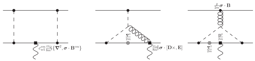
Figure 9: Some diagrams contributing to the matching at order $1/m^{3}$.

We focus on the operators (124) and (125). They come from matching spin-dependent NRQCD amplitudes that contain operators with at least two spatial derivatives (see Fig. 9). We have the following cases.

1. Amplitudes that are made of a $\mathcal{O}(1/m^{3})$ operator of NRQCD may couple to longitudinal photons, to photons embedded in covariant derivatives or to the magnetic fields of the operators. The first case is excluded, for only transverse photons contribute to the operators (124) and (125). The second case does not contribute to the operators (124) and (125), for spin-dependent $\mathcal{O}(1/m^{3})$ operators of NRQCD contain at most two covariant derivatives. The third case involves the NRQCD operators

$$\frac{c^{\textrm{em}}_{W1}}{8m^{3}}\psi^{\dagger}\{{\bf D}^{2},\mbox{\boldmath$\sigma$}\cdot ee_{Q}{\bf B}^{{\textrm{em}}}\}\psi-\frac{c^{\textrm{em}}_{W2}}{4m^{3}}\psi^{\dagger}{\bf D}^{i}\mbox{\boldmath$\sigma$}\cdot ee_{Q}{\bf B}^{{\textrm{em}}}{\bf D}^{i}\psi\,,$$ (126)

$$\frac{c^{\textrm{em}}_{p^{\prime}p}}{8m^{3}}\psi^{\dagger}\left(\mbox{\boldmath$\sigma$}\cdot{\bf D}\;ee_{Q}{\bf B}^{\textrm{em}}\cdot{\bf D}+{\bf D}\cdot ee_{Q}{\bf B}^{\textrm{em}}\;\mbox{\boldmath$\sigma$}\cdot{\bf D}\right)\psi\,,$$ (127)

and the corresponding c.c. ones, with $c^{\textrm{em}}_{W1}-c^{\textrm{em}}_{W2}=1$ and $c_{p^{\prime}p}^{{\textrm{em}}}={\cal O}(\alpha_{\textrm{s}})$ hep-ph/0512369 ; hep-ph/9701294 . For the purpose of matching the operators (124) and (125), the covariant derivatives may be replaced by simple derivatives that do not act on the gluon fields. We are, therefore, in the situation discussed in Sec. III.3, paragraph (iv), and Eq. (20) leads to

$$V^{\frac{\nabla_{r}^{2}\,\sigma\cdot B}{m^{3}}}=1,\qquad V^{\frac{(\nabla_{r}\cdot\sigma)\,(\nabla_{r}\cdot B)}{m^{3}}}=c_{p^{\prime}p}^{{\textrm{em}}}\,.$$ (128)

These relations are exact because, as we are going to detail in the following, NRQCD amplitudes with insertions of $1/m$ and $1/m^{2}$ operators factorize at relative order $v^{2}$ into contributions to $1/m$ and $1/m^{2}$ pNRQCD operators.

2. In diagrams made of a kinetic energy and a chromoelectric spin-orbit operator, the photon is coupled to one of the covariant derivatives. If it is coupled to the covariant derivative of the chromoelectric spin-orbit operator, then the two derivatives come from the kinetic energy operator, which factorizes. If it is coupled to the kinetic energy operator, then the photon field multiplies a derivative, the operator commutes with the gluons and factorizes.

3. The situation is similar for diagrams with a kinetic energy and an electric spin-orbit operator insertion.

4. In diagrams made of two kinetic energy and a chromomagnetic dipole operator, the photon is coupled to one of the kinetic energy operators. If the photon field multiplies a derivative, then either the operator commutes with the gluons and factorizes or it does not and then the two derivatives come from the other kinetic energy operator, which factorizes. If the photon field multiplies a gluon field then the two derivatives come from the other kinetic energy operator, which factorizes.

5. The kinetic energy operator also factorizes in diagrams with a magnetic and a chromomagnetic dipole operator.

6. Finally, in diagrams made of two kinetic energy and a magnetic dipole operator, the magnetic dipole operator commutes at relative order $v^{2}$ with the kinetic energy and factorizes.

We conclude therefore that (128) holds to any order of the matching, while only the Wilson coefficient $V^{\frac{\sigma\cdot B}{m^{3}}}$ of (36), the only operator without derivatives, may possibly get corrections from the matching beyond tree level.

References

- (1) N. Brambilla et al., CERN-2005-005, (CERN, Geneva, 2005) [arXiv:hep-ph/0412158].
- (2) N. Brambilla, S. Eidelman, B. K. Heltsley, R. Vogt, G. T. Bodwin, E. Eichten, A. D. Frawley and A. B. Meyer et al., Eur. Phys. J. C 71, 1534 (2011) [arXiv:1010.5827 [hep-ph]].
- (3) M. Ablikim et al. [BESIII Collaboration], Phys. Rev. Lett. 104, 132002 (2010) [arXiv:1002.0501 [hep-ex]].
- (4) B. Aubert et al. [BABAR Collaboration], Phys. Rev. Lett. 103, 161801 (2009) [arXiv:0903.1124 [hep-ex]].
- (5) G. Bonvicini et al. [CLEO Collaboration], Phys. Rev. D 81, 031104 (2010) [arXiv:0909.5474 [hep-ex]].
- (6) J. P. Lees et al. [The BABAR Collaboration], Phys. Rev. D 84, 091101 (2011) [arXiv:1102.4565 [hep-ex]]; R. Mizuk [BELLE Collaboration], talk at the QWG workshop, GSI, (2011).
- (7) M. Kornicer et al. [CLEO Collaboration], Phys. Rev. D 83, 054003 (2011) [arXiv:1012.0589 [hep-ex]].
- (8) J. P. Lees et al. [BABAR Collaboration], Phys. Rev. D 84, 072002 (2011) [Phys. Rev. D 84, 099901 (2011)] [arXiv:1104.5254 [hep-ex]].
- (9) K. Nakamura et al. [Particle Data Group Collaboration], J. Phys. GG 37, 075021 (2010).
- (10) H. Grotch, D. A. Owen and K. J. Sebastian, Phys. Rev. D 30, 1924 (1984).
- (11) E. Eichten, S. Godfrey, H. Mahlke and J. L. Rosner, Rev. Mod. Phys. 80, 1161 (2008) [hep-ph/0701208].
- (12) N. Brambilla, A. Pineda, J. Soto and A. Vairo, Rev. Mod. Phys. 77, 1423 (2005) [hep-ph/0410047].
- (13) N. Brambilla, Y. Jia and A. Vairo, Phys. Rev. D 73, 054005 (2006) [hep-ph/0512369].
- (14) P. Pietrulewicz, Effective field theory for electromagnetic transitions of heavy quarkonium, Diploma Thesis (Munich, 2011).
- (15) W. E. Caswell and G. P. Lepage, Phys. Lett. B 167, 437 (1986).
- (16) G. T. Bodwin, E. Braaten and G. P. Lepage, Phys. Rev. D 51, 1125 (1995) [Erratum-ibid. D 55, 5853 (1997)] [hep-ph/9407339].
- (17) A. Pineda and J. Soto, Nucl. Phys. Proc. Suppl. 64, 428 (1998) [hep-ph/9707481].
- (18) N. Brambilla, A. Pineda, J. Soto and A. Vairo, Nucl. Phys. B 566, 275 (2000) [hep-ph/9907240].
- (19) M. E. Luke and A. V. Manohar, Phys. Lett. B 286, 348 (1992) [hep-ph/9205228].
- (20) A. V. Manohar, Phys. Rev. D 56, 230 (1997) [hep-ph/9701294].
- (21) N. Brambilla, X. Garcia i Tormo, J. Soto and A. Vairo, Phys. Rev. D 80 (2009) 034016 [arXiv:0906.1390 [hep-ph]].
- (22) N. Brambilla, A. Pineda, J. Soto and A. Vairo, Phys. Rev. D 63, 014023 (2001) [hep-ph/0002250].
- (23) A. Pineda and A. Vairo, Phys. Rev. D 63, 054007 (2001) [Erratum-ibid. D 64, 039902 (2001)] [hep-ph/0009145].
- (24) D. Eiras and J. Soto, Phys. Lett. B 491, 101 (2000) [hep-ph/0005066].
- (25) N. Brambilla, Y. Sumino and A. Vairo, Phys. Rev. D 65, 034001 (2002) [hep-ph/0108084].
- (26) N. Brambilla, D. Gromes and A. Vairo, Phys. Lett. B 576, 314 (2003) [hep-ph/0306107].
- (27) Y. Jia, W. -L. Sang and J. Xu, arXiv:1007.4541 [hep-ph].
- (28) E. Eichten, K. Gottfried, T. Kinoshita, K. D. Lane and T. -M. Yan, Phys. Rev. D 17, 3090 (1978) [Erratum-ibid. D 21, 313 (1980)].
- (29) N. Brambilla, A. Pineda, J. Soto and A. Vairo, Phys. Lett. B 470, 215 (1999) [hep-ph/9910238].
- (30) H. A. Bethe and E. E. Salpeter, Quantum Mechanics of One and Two-Electron Atoms (Plenum, New York, 1977).
- (31) Y. Koma, M. Koma and H. Wittig, Phys. Rev. Lett. 97, 122003 (2006) [arXiv:hep-lat/0607009].
- (32) Y. Koma and M. Koma, Nucl. Phys. B 769, 79 (2007) [arXiv:hep-lat/0609078].
- (33) Y. Koma, M. Koma and H. Wittig, PoS LAT2007, 111 (2007) [arXiv:0711.2322 [hep-lat]].
- (34) A. Laschka, N. Kaiser and W. Weise, Phys. Rev. D 83, 094002 (2011) [arXiv:1102.0945 [hep-ph]].
- (35) G. D. Kribs, T. S. Roy, J. Terning and K. M. Zurek, Phys. Rev. D 81, 095001 (2010) [arXiv:0909.2034 [hep-ph]].