Gakuto International Series
Mathematical Sciences and Applications (2011)
in press

THE STUDY OF MACROSCOPIC DYNAMICS OF NANO PROCESSES IN BALL MILLS THROUGH NANO-SCALE SIMULATION

Abstract. Numerical simulation for comminution processes inside the vial of ball mills are performed using Monte Carlo method. The internal dynamics is represented by recently developed model based on hamiltonian involving the impact and surrounding electromagnetic potentials. The paper is focused on investigating the behaviors of normalized macroscopic pressure, $P/{P_{0}}$, in term of system temperature and the milled powder mass. The results provide theoretical justification that high efficiency is expected at low system temperature region. It is argued that keeping the system temperature as low as possible is crucial to prevent agglomeration which is a severe obstacle for further comminution processes.
Keywords: comminution, modeling, ball mill, hamiltonian, canonical ensemble

——————————————————————————
Received xxxxxxxxxx, 2011.
This work is supported by Riset Kompetitif LIPI FY 2010.
AMS Subject Classification 70-08,70F99

1 Introduction

Ball mills have been deployed as a simple top-down approach for comminution processes up to nanometer scale. Although its practicality, ball mills involve many parameters related to both external and internal dynamics of the equipments. All of them unfortunately lead to severe uncertainties and become some major obstacles to perform an efficient milling.

Meanwhile, more theoretical approaches based on mathematical description are expected to overcome such problems. Many efforts have been done to develop modelization of ball mill equipments [1, 2, 3, 4, 5]. Through the modeling approach and its subsequent simulation, one expects to be able to obtain prior information and constraints to optimize experimental strategy.

In general, the experimental works using ball mill equipments face the following problems :

• Choosing an appropriate parameter set related to the milled materials for particular case of experiments. It could be the ball size, the initial size of milled powders, the number of ball, the initial quantity of powders, material characteristics of ball and also powders, and so forth.

• The milling time for particular characteristics and quantities of balls and powders.

• The design and geometrical motions of vial itself. Although there are various types of ball mills, most of them have not been developed based on prior comprehensive simulations.

• On the other hand, the experimental measurements on the internal dynamics of vial are almost impossible.

The question is then how to overcome these problems ? Is there any smart solution for these obstacles ?

In our recent works, a novel model to describe the internal dynamics and to relate it with surrounding environment has been proposed [6, 7]. In contrast to the semi-empirical approaches, the model does not require prior experimental data or simulation results to fit the parameters [8, 9, 10, 11], nor huge computational power as in some more empirical approaches [12, 13, 14]. Actually our model combines the deterministic approach for milling bodies motion, and the statistical approach to relate them with external macroscopic physical observables, in particular system temperature.

In this paper, however the focus is put on investigating the behaviors of normalized macroscopic pressure, $P/{P_{0}}$. The observable is important and accessible in most of real experiments. Particular interest is investigating its dependencies on the system temperature and the evolution milled powder mass as well.

The paper is organized as follows. First, after this introduction the model is briefly explained. Before summarizing the results, numerical analysis and simulation for the normalized pressure in term of system temperature are discussed.

2 Model and simulation

Rather solving a set of equation of motions (EOMs) governing the whole dynamics as always done in conventional approaches, the dynamics is described in a hamiltonian involving all considerable potentials in the system and its surrounding environment.

In the model, the dynamics of each ’matter’ in the system, i.e. balls and powders inside the vial, are described by a hamiltonian $H_{\mathrm{m}}(\vec{r},t)$. The index $\mathrm{m}$ denotes the powder ($\mathrm{p}$) or ball ($\mathrm{b}$) and $\vec{r}=(x,y,z)$. The hamiltonian contains some terms representing all relevant interactions working on the matters inside the system as follow [7],

$$H_{\mathrm{m}}=H_{0}+V_{\mathrm{m}-\mathrm{m}}+V_{\mathrm{m}-\mathrm{v}}+V_{\mathrm{m}-\mathrm{m}^{\prime}}+V_{\mathrm{ext}}\;,$$ (1)

with $\mathrm{v}$ denotes the vial, while $H_{0}$ is the free matter hamiltonian containing the kinetic term,

$$H_{0}=\frac{1}{2m_{\mathrm{m}}}\sum_{i=1}^{n_{\mathrm{m}}}\left|\left(\vec{p}_{\mathrm{m}}\right)_{i}\right|^{2}\;,$$ (2)

where $n_{\mathrm{m}}$ is the matter number, $m_{\mathrm{m}}$ and $\vec{p}_{\mathrm{m}}$ are the matter mass and momentum respectively. Throughout the paper we assume that the mass or size evolution of matters is uniform for the same matters.

The matter self-interaction $V_{\mathrm{m}-\mathrm{m}}$, the matter–vial interaction $V_{\mathrm{m}-\mathrm{v}}$ and the interactions between different matters may be induced by, for instance, the impact ($V^{\mathrm{imp}}$) potential,

$$V^{\mathrm{imp}}_{\mathrm{m}-{\mathrm{m}^{\prime}}}(\vec{r},t) = -\sum_{i=1}^{n_{\mathrm{m}}}\sum_{j=1}^{n_{\mathrm{m}^{\prime}}}\int_{0}^{\left(\xi_{\mathrm{m}{\mathrm{m}^{\prime}}}\right)_{ij}}\mathrm{d}\left(\xi_{\mathrm{m}{\mathrm{m}^{\prime}}}\right)_{ij}\,\vec{n}\cdot\left(\vec{F}^{\mathrm{imp}}_{\mathrm{m}{\mathrm{m}^{\prime}}}\right)_{ij}\;,$$ (3)

with $\mathrm{m},{\mathrm{m}^{\prime}}:\mathrm{v},\mathrm{p},\mathrm{b}$ and $\vec{n}$ is the unit normal vector. The potential should in fact represent the whole classical dynamics among the matters, i.e. the impact forces among balls and powders. Here the impact force is dominated by its normal component [14],

$$\vec{F}^{\mathrm{imp}}_{\mathrm{m}{\mathrm{m}^{\prime}}}(\vec{r},t)=\left[\frac{2\Upsilon_{\mathrm{m}{\mathrm{m}^{\prime}}}}{3(1-v_{\mathrm{m}{\mathrm{m}^{\prime}}}^{2})}\sqrt{R_{\mathrm{m}{\mathrm{m}^{\prime}}}^{\mathrm{eff}}}\left(\xi_{\mathrm{m}{\mathrm{m}^{\prime}}}^{{3}/{2}}+\frac{3}{2}A_{\mathrm{m}{\mathrm{m}^{\prime}}}\sqrt{\xi_{\mathrm{m}{\mathrm{m}^{\prime}}}}\,\frac{\mathrm{d}\xi_{\mathrm{m}{\mathrm{m}^{\prime}}}}{\mathrm{d}t}\right)\right]\vec{n}\;.$$ (4)

Here, $\Upsilon_{\mathrm{m}{\mathrm{m}^{\prime}}}$ is the Young modulus, $v_{\mathrm{m}{\mathrm{m}^{\prime}}}$ represents the Poisson ratio of the sphere material, $R_{\mathrm{m}{\mathrm{m}^{\prime}}}^{\mathrm{eff}}={(R_{\mathrm{m}}R_{\mathrm{m}^{\prime}})}/{(R_{\mathrm{m}}+R_{\mathrm{m}^{\prime}})}$ is the effective radius, while $\xi_{\mathrm{m}{\mathrm{m}^{\prime}}}=R_{\mathrm{m}}+R_{\mathrm{m}^{\prime}}-|\vec{r}_{\mathrm{m}}-\vec{r}_{\mathrm{m}^{\prime}}|$ is the displacement with $R_{\mathrm{m}}$ is the radius of interacting matter. $A$ is a dissipative parameter given in [15, 16, 17] containing the viscous constant $\eta_{\mathrm{m}}$.

In fact, there are another potentials like Coulomb and gravitational potentials which may influence on the system. However, those contributions should be considerably tiny due to its neutral charges and tiny masses as well [7].

Incorporating the effect of external electromagnetic field surrounding the system for charged matters shifts the kinetic term in Eq. 2 to be [7],

$$H_{0}\longrightarrow H_{0+\mathrm{EM}}=\frac{1}{2m_{\mathrm{m}}}\sum_{i=1}^{n_{\mathrm{m}}}\left|\left(\vec{p}_{\mathrm{m}}\right)_{i}-Q_{\mathrm{m}}\,\vec{A}\right|^{2}+n_{\mathrm{m}}\,Q_{\mathrm{m}}\,\phi\;,$$ (5)

with electromagnetic (scalar and vector) potential $(\phi,\vec{A})$ and the matter charge $Q_{\mathrm{m}}$.

From now, let us focus only on the dynamics of powders which is our main interest in the sense of comminution process. From Eqs. (1), (2) and (3), the total hamiltonian for the powder in the model is,

$$H_{\mathrm{p}} = \frac{1}{2m_{\mathrm{p}}}\sum_{i=1}^{n_{\mathrm{p}}}\left|\left(\vec{p}_{\mathrm{p}}\right)_{i}-Q_{\mathrm{p}}\,\vec{A}\right|^{2}+n_{\mathrm{p}}\,Q_{\mathrm{p}}\,\phi$$ (6)

$$-\frac{1}{2}\sum_{i(\neq j)=1}^{n_{\mathrm{p}}}\sum_{j=1}^{n_{\mathrm{p}}}\int_{0}^{\left(\xi_{\mathrm{p}\mathrm{p}}\right)_{ij}}\mathrm{d}\left(\xi_{\mathrm{p}\mathrm{p}}\right)_{ij}\,\vec{n}\cdot\left(\vec{F}^{\mathrm{imp}}_{\mathrm{p}\mathrm{p}}\right)_{ij}$$

$$-\sum_{m:\mathrm{b},\mathrm{v}}\sum_{i=1}^{n_{\mathrm{p}}}\sum_{j=1}^{n_{\mathrm{m}}}\int_{0}^{\left(\xi_{\mathrm{p}\mathrm{m}}\right)_{ij}}\mathrm{d}\left(\xi_{\mathrm{p}\mathrm{m}}\right)_{ij}\,\vec{n}\cdot\left(\vec{F}^{\mathrm{imp}}_{\mathrm{p}\mathrm{m}}\right)_{ij}\;,$$

for $Q_{\mathrm{p}}\neq 0$. The last two potentials represent the total impact potential among powders; powders and vial; powders and balls respectively. Obviously we do not need to take into account the ball self-interaction $V^{\mathrm{imp}}_{\mathrm{b}-\mathrm{b}}$ nor ball-vial interaction $V^{\mathrm{imp}}_{\mathrm{b}-\mathrm{v}}$. This is actually the advantage of using hamiltonian method.

Relating a hamiltonian with macroscopic physical observables can be realized through the partition function known in statistical mechanics,

$$Z_{\mathrm{m}}=\int\prod_{i=1}^{n_{\mathrm{m}}}\mathrm{d}\vec{p}_{i}\,\mathrm{d}\vec{r}_{i}\;\mathrm{exp}\left[-\int_{0}^{\beta}\mathrm{d}t\,H_{\mathrm{m}}\right]\;,$$ (7)

for a canonical ensemble of matter m governed by a particular hamiltonian $H_{\mathrm{m}}$. Here, $\beta\equiv 1/{(k_{B}T)}$ with $k_{B}$ and $T$ are the Boltzman constant and absolute temperature. Further one can calculate, for instance the normalized pressure as,

$$P^{\prime}_{\mathrm{m}}=\frac{\ln Z_{\mathrm{m}}}{\ln{Z_{0}}_{\mathrm{m}}}\;.$$ (8)

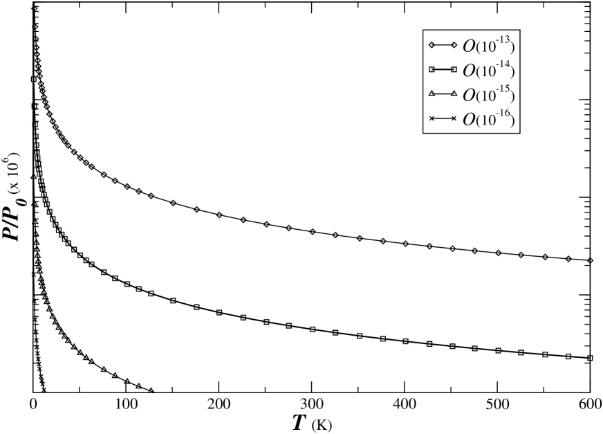
Figure 1: The normalized macroscopic pressure, $P/{P_{0}}$, as a function of temperature for typical order values of ${\cal F}=O(10^{-13})\sim O(10^{-16})$.

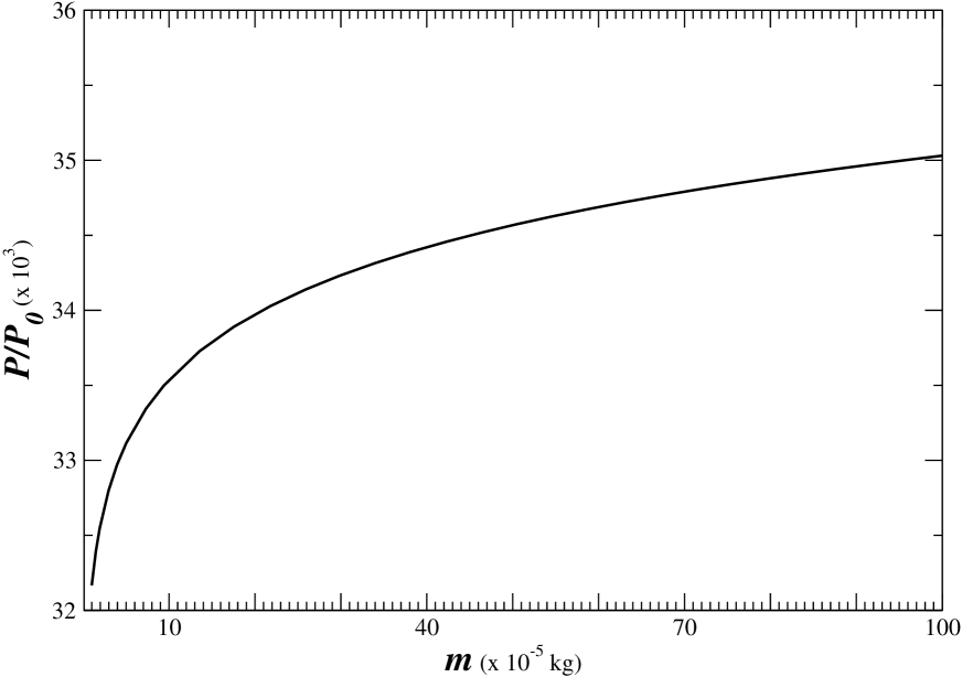
Figure 2: The normalized macroscopic pressure, $P/{P_{0}}$, as a function of powder mass for ${\cal F}\sim O(10^{-14})$ at typical room temperature.

Integrating out the time component at finite temperature, one obtains [7],

$$P^{\prime}_{\mathrm{p}}=1-\beta\,{\cal F}\,\ln^{-1}\left(\frac{2\,m_{\mathrm{p}}\pi}{\beta}\right)\;,$$ (9)

respectively with,

$${\cal F} \equiv 2\,\int\prod_{i=1}^{n_{\mathrm{p}}}\mathrm{d}\vec{r}_{i}\left[Q_{\mathrm{p}}\,\phi-\frac{2}{15\,n_{\mathrm{p}}}\sum_{i(\neq j)=1}^{n_{\mathrm{p}}}\sum_{j=1}^{n_{\mathrm{p}}}\frac{\Upsilon_{\mathrm{p}\mathrm{p}}}{1-v_{\mathrm{p}\mathrm{p}}^{2}}\sqrt{R_{\mathrm{p}\mathrm{p}}^{\mathrm{eff}}}\,\left(\xi_{\mathrm{p}\mathrm{p}}\right)_{ij}^{{5}/{2}}\right.$$ (10)

$$\left.-\frac{4}{15\,n_{\mathrm{p}}}\sum_{\mathrm{m}:\mathrm{b},\mathrm{v}}\sum_{i=1}^{n_{\mathrm{p}}}\sum_{j=1}^{n_{\mathrm{m}}}\frac{\Upsilon_{\mathrm{p}\mathrm{m}}}{1-v_{\mathrm{p}\mathrm{m}}^{2}}\sqrt{R_{\mathrm{p}\mathrm{m}}^{\mathrm{eff}}}\,\left(\xi_{\mathrm{p}\mathrm{m}}\right)_{ij}^{{5}/{2}}\right]\;.$$

Eq. (9) provides a general behavior for temperature-dependent pressure in the model, while the geometrical structure and motion of vial is absorbed in the function ${\cal F}$.

This is the final result which is ready to be evaluated further using numerical approaches like Monte Carlo.

3 Results and summary

In this paper, the integral in Eq. (10) is performed using Monte Carlo technique. Simulation on the system temperature dependencies of normalized pressure is shown in Fig. 1. Secondly its dependencies on matter mass is given in Fig. 2.

The simulation is done for steel material in a typical geometry of spex mixer / mill with resolutions on 3-dimensional space $\sim 10^{4}\times 10^{4}\times 10^{4}$, vial length $l=50$ mm, vial radius $r_{\mathrm{v}}=10$ mm, shaft-arm length $L=200$ mm and ball radius $R_{\mathrm{b}}=5$ mm.

From the figures one can conclude that high efficiency is expected at low system temperature region as can be understood from natural sense since the higher is temperature, the agglomeration phenomena occurs which prevents further comminution processes. In another words, the higher is temperature, the pressure is getting down which lead to lower impact energy. Therefore these results suggest that in general one should keep optimized working temperature as long as possible to keep high energy milling.

References

- [1] B. K. Mishra and R. K. Rajamani. The discrete element method for the simulation of ball mills. Applied Mathematical Modeling, 16:598–604, 1992.
- [2] B. K. Mishra and R. K. Rajamani. Simulation of charge motion in ball mills. International Journal of Mineral Processing, 40:171–186, 1994.
- [3] B. K. Mishra. Charge dynamics in planetary mill. Kona Powder Particle, 13:151–158, 1995.
- [4] B. K. Mishra and C. V. R. Murty. On the determination of contact parameters for the realistic DEM simulations of ball mills. Powder Technology, 115:290–297, 2001.
- [5] T. Pschel and C. Saluea. Scaling properties of granular materials. Physical Review, E64:011308, 2001.
- [6] Muhandis, F. N. Diana, A. S. Wismogroho, N. T. Rochman, and L. T. Handoko. Extracting physical observables using macroscopic ensemble in the spex-mixer/mill simulation. AIP Conference Proceeding, 1169:235–240, 2009.
- [7] G. K. Sunnardianto, Muhandis, F. N. Diana, and L. T. Handoko. Modeling comminution processes in ball mills as a canonical ensemble. Journal of Computational and Theoretical Nanoscience, 8:124–132, 2011.
- [8] G. Manai, F. Delogu, and M. Rustici. Onset of chaotic dynamics in a ball mill : atractor merging and crisis induced intermittency. Chaos, 12:601–609, 2002.
- [9] R. M. Davis, B. McDermott, and C. C. Koch. Mechanical alloying of brittle materials. Metallurgical Transactions, A19:2867, 1988.
- [10] D. Maurice and T. H. Courtney. The physics of mechanical alloying : a first report. Metallurgical Transactions, A21:289–302, 1990.
- [11] D. Maurice and T. H. Courtney. Milling dynamics, Part II : dynamic of a spex mill in a one dimensional mill. Metallurgical Transactions, A27:1981, 1996.
- [12] F. Delogu, M. Monagheddu, G. Mulas, L. Schiffini, and G. Cocco. Impact characteristics and mechanical alloying processes by ball milling. Innternational Journal of Non-Equilibrium Processing, 11:235–269, 2000.
- [13] W. Wang. Modeling and simulation of the dynamics process in high energy ball milling of metal powders. PhD thesis, University of Waikato, 2000.
- [14] A. Concas, N. Lai, M. Pisu, and G. Cao. Modelling of comminution processes in spex mixer/mill. Chemical Engineering Science, 61:3746–3760, 2006.
- [15] N. V. Brilliantov, Frank Spahn, Jan Martin Hertzsch, and Thorsten Pschel. Model for collision in granular gases. Physical Review, E53:5382–5392, 1996.
- [16] L. D. Landau and E. M. Lifschitz. Theory of Elasticity. Oxford University Press, 1965.
- [17] H. Hertzsch, F. Sepahan, and N. V. Brilliantov. On low-veklocity collisions of viscoelastic particles. Journal de Physique, 5:1725–1738, 1995.