APEX-CHAMP⁺ high-$J$ CO observations of
low–mass young stellar objects:

Abstract

Context. The NGC 1333 IRAS 4A and IRAS 4B sources are among the best studied Stage 0 low-mass protostars which are driving prominent bipolar outflows. Spectrally resolved molecular emission lines provide crucial information regarding the physical and chemical structure of the circumstellar material as well as the dynamics of the different components. Most studies have so far concentrated on the colder parts ($T$ $\leq$30 K) of these regions.

Aims. The aim is to characterize the warmer parts of the protostellar envelope using the new generation of submillimeter instruments. This will allow us to quantify the feedback of the protostars on their surroundings in terms of shocks, UV heating, photodissociation and outflow dispersal.

Methods. The dual frequency 2$\times$7 pixel 650/850 GHz array receiver CHAMP⁺ mounted on APEX was used to obtain a fully sampled, large-scale $\sim$4$\arcmin\times 4\arcmin$ map at 9$\arcsec$ resolution of the IRAS 4A/4B region in the ¹²CO $J$=6–5 line. Smaller maps are observed in the ¹³CO 6–5 and [C i] $J$=2–1 lines. In addition, a fully sampled ¹²CO $J$=3–2 map made with HARP-B on the JCMT is presented and deep isotopolog observations are obtained at selected outflow positions to constrain the optical depth. Complementary Herschel-HIFI and ground-based lines of CO and its isotopologs, from $J$=1–0 up to 10–9 ($E_{\rm u}/k\approx$300 K), are collected at the source positions and used to construct velocity resolved CO ladders and rotational diagrams. Radiative-transfer models of the dust and lines are used to determine temperatures and masses of the outflowing and photon-heated gas and infer the CO abundance structure.

Results. Broad CO emission line profiles trace entrained shocked gas along the outflow walls, with typical temperatures of $\sim$100 K. At other positions surrounding the outflow and the protostar, the 6–5 line profiles are narrow indicating UV excitation. The narrow ¹³CO 6-5 data directly reveal the UV heated gas distribution for the first time. The amount of UV-photon-heated gas and outflowing gas are quantified from the combined ¹²CO and ¹³CO 6–5 maps and found to be comparable within a 20$\arcsec$ radius around IRAS 4A, which implies that UV photons can affect the gas as much as the outflows. Weak [C I] emission throughout the region indicates a lack of CO dissociating photons. Modeling of the C¹⁸O lines indicates the necessity of a “drop” abundance profile throughout the envelopes where the CO freezes out and is reloaded back into the gas phase through grain heating, thus providing quantitative evidence for the CO ice evaporation zone around the protostars. The inner abundances are less than the canonical value of CO/H₂=2.7$\times 10^{-4}$, however, indicating some processing of CO into other species on the grains. The implications of our results for the analysis of spectrally unresolved Herschel data are discussed.

1 Introduction

In the very early stages of star formation, newly forming protostars are mainly characterized by their large envelopes ($\sim$10⁴ AU in diameter) and bipolar outflows (Lada 1987; Greene et al. 1994). As gas and dust from the collapsing core accrete onto the central source, the protostar drives out material along both poles at supersonic speeds to distances up to a parsec or more. Outflows have a significant impact on their surroundings, by creating shock waves which increase the temperature and change the chemical composition (Snell et al. 1980; Bachiller & Tafalla 1999; Arce et al. 2007). By sweeping up material, they carry off envelope mass and limit the growth of the protostar. They also create a cavity through which ultraviolet photons from the protostar can escape and impact the cloud (Spaans et al. 1995). Quantifying these active ‘feedback’ processes and distinguishing them from the passive heating of the inner envelope by the protostellar luminosity is important for a complete understanding of the physics and chemistry during protostellar evolution.

Most studies of low-mass protostars to date have used low-excitation lines of CO and isotopologs ($J_{\rm u}$ $\leq$ 3) combined with dust continuum mapping to characterize the cold gas in envelopes and outflows (e.g., Blake et al. 1995; Bontemps et al. 1996; Shirley et al. 2002; Robitaille et al. 2006). A wealth of other molecules has also been observed at mm wavelengths, but their use as temperature probes is complicated by the fact that they also have large abundance gradients through the envelope driven by release of ice mantles (e.g., van Dishoeck & Blake 1998; Ceccarelli et al. 2007; Bottinelli et al. 2007). Moreover, molecules with large dipole moments such as CH₃OH are often highly subthermally excited unless densities are very high (e.g. Bachiller et al. 1995; Johnstone et al. 2003). With the opening up of high-frequency observations from the ground and in space, higher excitation lines of CO can now be routinely observed so that their diagnostic potential as temperature and column density probes can now be fully exploited.

Tracing warm gas with CO up to $J$=7–6 from the ground requires the best atmospheric conditions, as well as state-of-art detectors. The combination is offered by the CHAMP⁺ 650/850 GHz 2$\times$7 pixel array receiver (Kasemann et al. 2006) currently mounted at the Atacama Pathfinder EXperiment (APEX) Telescope at 5100 m altitude on Cerro Chajnantor (e.g. Güsten et al. 2008). Moreover, the spectroscopic instruments on the Herschel Space Observatory have the sensitivity to observe CO lines up to $J$=44–43 unhindered by the Earth’s atmosphere, even for low-mass young stellar objects (e.g., van Kempen et al. 2010a, b; Lefloch et al. 2010; Yıldız et al. 2010). Together, these data allow to address questions such as (i) How is CO excited, is it due to shock or UV heating? (ii) How much warm gas is present in the inner regions of the protostellar envelopes and from which location does it originate? What is the swept up mass and how warm is it? (iii) What is the CO abundance structure throughout the envelope: where is CO frozen out and where is it processed?

Over the past several years, our group has conducted a survey of APEX-CHAMP⁺ mapping of high$-J$ lines of CO and isotopologs of embedded low-mass Stage 0 and 1 (cf. nomenclature by Robitaille et al. 2006) young stellar objects (YSOs) (van Kempen et al. 2009a, b, c, Paper I and II in this series). These data complement our earlier surveys at lower frequency of CO and other molecules with the James Clerk Maxwell Telescope (JCMT), IRAM 30m, APEX and Onsala telescopes (e.g., Jørgensen et al. 2002, 2004; van Kempen et al. 2009c). More recently, the same sources are being observed with the Herschel Space Observatory in the context of the ‘Water in star-forming regions with Herschel’ (WISH) key program (van Dishoeck et al. 2011). The ¹²CO $J$=6–5 ($E_{\rm u}/k$=115 K) line is particularly useful in tracing the outflows through broad line wings, complementing recent mapping in the ¹²CO $J$=3–2 line with the HARP-B array on the JCMT (e.g., Curtis et al. 2010b). The availability of lines up to CO $J$=7–6 gives much better constraints on the excitation temperature of the gas, which together with the higher angular resolution of the high frequency data should result in more accurate determination of outflow properties such as the force and momentum.

In addition to broad line wings, van Kempen et al. (2009b) also found narrow extended ¹²CO 6–5 emission along the cavity walls. Combined with narrow ¹³CO 6–5 emission, this was interpreted as evidence for UV photon-heated gas, following earlier work by Spaans et al. (1995). The mini-survey by van Kempen et al. (2009c) found this narrow extended emission to be ubiquitous in low-mass protostars. Further evidence for UV photon heating was provided by far-infrared CO lines with $J_{\rm u}$=10 to 20 observed with Herschel-PACS (van Kempen et al. 2010b; Visser et al. 2011). However, Herschel has only limited mapping capabilities; PACS lacks velocity resolution and HIFI has a quite large beam (20″– 40″). Thus, large scale velocity resolved maps at $<10^{\prime\prime}$ resolution as offered by APEX-CHAMP⁺ form an important complement to the Herschel data. In this paper, we present fully sampled high-$J$ CHAMP⁺ maps of one of the largest and most prominent low-mass outflow regions, NGC 1333 IRAS 4.

NGC 1333 IRAS 4A and IRAS 4B (hereafter only IRAS 4A and IRAS 4B) are two low-mass protostars in the southeast corner of the NGC 1333 region (see Walawender et al. 2008, for review). They have attracted significant attention due to their strong continuum emission, powerful outflows and rich chemistry (André & Montmerle 1994; Blake et al. 1995; Bottinelli et al. 2007). They were first identified as water maser spots by Ho & Barrett (1980) and later confirmed as protostellar candidates by IRAS observations (Jennings et al. 1987) and resolved individually in JCMT-SCUBA submm continuum maps (Sandell et al. 1991; Sandell & Knee 2001; Di Francesco et al. 2008). Using mm interferometry, it was subsequently found that both protostars are in proto-multiple systems (Lay et al. 1995; Looney et al. 2000). The projected separation between IRAS 4A and IRAS 4B is 31$\arcsec$ ($\sim$7500 AU). The companion to IRAS 4B is clearly detected at a separation of 11$\arcsec$ whereas that of IRAS 4A has a separation of only 2$\arcsec$ (Jørgensen et al. 2007). The distance to the NGC 1333 nebula is still in debate (see Curtis et al. 2010a, for more thorough discussions). In this paper, we adopt the distance of 235$\pm$18 pc based on VLBI parallax measurements of water masers in SVS 13 in the same cluster (Hirota et al. 2008).

We here present an APEX-CHAMP^{+ 12}CO 6–5 map over a $4^{\prime}\times 4^{\prime}$ area at 9^′′ resolution, together with ¹³CO 6–5 and [C i] $J$=2–1 maps over a smaller region ($1^{\prime}\times 1^{\prime}$). Moreover, ¹³CO 8–7 and C¹⁸O 6–5 lines are obtained at the central source positions. These data are analyzed together with the higher-$J$ Herschel-HIFI observations of CO and isotopologs recently published by Yıldız et al. (2010) as well as lower-$J$ JCMT, IRAM 30m and Onsala archival data so that spectrally resolved information on nearly the entire CO ladder up to 10–9 ($E_{\rm u}/k$=300 K) is obtained for all three isotopologs. The spectrally resolved data allow the temperatures in different components to be determined, and thus provide an important complement to spectrally unresolved Herschel PACS and SPIRE data of the CO ladder of such sources. In addition, a new JCMT HARP-B map of ¹²CO 3–2 has been obtained over the same area, as well as deep ¹³CO spectra at selected outflow positions to constrain the optical depth. The APEX-CHAMP⁺ and JCMT maps over a large area can test the interpretation of the different velocity components seen in HIFI data which has so far been based only on single position data.

The outline of the paper is as follows. In Section 2, the observations and the telescopes where the data have been obtained are described. In Section 3, the inventory of complementary lines and maps are presented. In Section 4, the data are analyzed to constrain the temperature and mass of the molecular outflows. In Section 5, the envelope abundance structure of these protostars is discussed. In Section 6, the amount of shocked gas is compared quantitatively to that of photon-heated gas. In Section 7, the conclusions from this work are summarized.

2 Observations

Table 4 gives a brief overview of the IRAS 4A and 4B sources. Spectral line data have been obtained primarily from the 12-m sub-mm Atacama Pathfinder Experiment Telescope, APEX (Güsten et al. 2008) at Llano de Chajnantor in Chile. In addition, we present new and archival results from the 15-m James Clerk Maxwell Telescope, JCMT at Mauna Kea, Hawaii; the 3.5-m Herschel Space Observatory (Pilbratt et al. 2010) and IRAM 30m telescope. Finally, we use published data from the Onsala 20-m and 14-m Five College Radio Astronomy Observatory, FCRAO telescopes.

Table 1: Source properties

Source	RA(J2000)	Dec(J2000)	Distance	$L_{\rm bol}$	$V_{\rm LSR}$
	[${}^{\mathrm{h}}\,{}^{\mathrm{m}}\,{}^{\mathrm{s}}$]	[$\degr\,\arcmin\,\arcsec$]	[pc]	[$L_{\odot}$]	[km s-1]
IRAS 4A	03 29 10.5	+31 13 30.9	235	9.1	+7.0
IRAS 4B	03 29 12.0	+31 13 08.1	235	4.4	+7.1

APEX: The main focus of this paper is the high-$J$ CO 6–5 and [C i] 2–1 maps of IRAS 4A and 4B, obtained with APEX-CHAMP⁺ in November 2008 and August 2009. The protostellar envelopes and their complete outflowing regions have been mapped in CO 6–5 emission using the on-the-fly mapping mode acquiring more than 100 000 spectra in 1.5 hours covering a Nyquist sampled 240$\arcsec\times$240$\arcsec$ region. The instrument consists of 2 heterodyne receiver arrays, each with 7 pixel detector elements for simultaneous operations in the 620–720 GHz and 780–950 GHz frequency ranges (Kasemann et al. 2006; Güsten et al. 2008). The following two lines were observed simultaneously: ¹²CO 6–5 and [C i] 2–1 (large map); ¹³CO 6–5 and [C i] 2–1 (smaller map); C¹⁸O 6–5 and ¹³CO 8–7 (staring at source positions); and ¹²CO 6–5 and ¹²CO 7–6 (staring at source positions).

The APEX beam sizes correspond to 8$\arcsec$ ($\sim$1900 AU at a distance of 235 pc) at 809 GHz and 9$\arcsec$ ($\sim$2100 AU) at 691 GHz. The observations were completed under excellent weather conditions (Precipitable Water Vapor, PWV $\sim$0.5 mm) with typical system temperatures of 1900 K for CHAMP⁺-I (SSB, 691 GHz), and 5600 K for CHAMP⁺-II (SSB, 809 GHz). The relatively high system temperatures are due to the high atmospheric pathlength at the low elevation of the sources of $\sim$25$\degr$. Also, for CHAMP⁺-II, there is a significant contribution from the receiver temperature. The observations were done using position-switching toward an emission free reference position in settings ¹²CO 6–5 + [C i] 2–1 or CO 7–6, and ¹³CO 6–5 + [C i] 2–1. However, in the setting C¹⁸O 6–5 and ¹³CO 8–7, a beam-switching of +/–90$\arcsec$ is used in staring mode in order to increase the $S/N$ on the central pixel (van Dishoeck et al. 2009). The CHAMP⁺ array uses the Fast Fourier Transform Spectrometer (FFTS) backend (Klein et al. 2006) for all seven pixels with a resolution of 0.12 MHz (0.045 km s^-1 at 800 GHz).

JCMT: A CO 3–2 fully sampled map is obtained from the JCMT with the HARP-B instrument in March 2010. HARP-B consists of 16 SIS detectors with 4$\times$4 pixel elements of 15$\arcsec$ each at 30$\arcsec$ separation. The opacity at the time of observations was excellent ($\tau_{\rm 225GHz}<$0.04) and the on-the-fly method was used to fully cover the entire outflow. Apart from the maps, line data of CO and isotopologs (e.g., 2–1 and 3–2 lines) were obtained from the JCMT and its public archive. In Table 7, the offset values of the archival data from the protostellar source coordinates are provided. In addition, we observed four distinct outflow knots of IRAS 4A in deep ¹²CO and ¹³CO 2–1 integrations to constrain the optical depth (see Table 7 for coordinates). The B1 and R1 positions are the blue and red-shifted outflow knots closest to IRAS 4A and B2 and R2 are the two prominent dense outflow knots further removed.

Herschel: Spectral lines of ¹²CO 10–9, ¹³CO 10–9, C¹⁸O 5–4, 9–8 and 10–9 were observed with the Herschel Space Observatory using the Heterodyne Instrument for Far-Infrared (HIFI); (de Graauw et al. 2010). All observations were done in dual-beam-switch (DBS) mode with a chop reference position located 3$\arcmin$ from the source positions. Except for the C¹⁸O 10–9 spectra, these data were presented in Yıldız et al. (2010) and observational details can be found there.

IRAM-30m: The lower-$J$ ¹³CO 1–0 and C¹⁷O 2–1 transitions were observed with the IRAM 30-m telescope by Jørgensen et al. (2002) and Pagani et al. (in prep).

Onsala: The lowest-$J$ C¹⁷O and C¹⁸O 1–0 transitions were observed with the Onsala 20-m radiotelescope by Jørgensen et al. (2002), and the spectra are used here.

FCRAO: ¹²CO 1–0 spectrum of IRAS 4A is extracted from COMPLETE survey map (Arce et al. 2010) observed with FCRAO.

Table 2: Overview of the observations of IRAS 4A and IRAS 4B

Source	Mol.	Trans.	$E_{\rm u}$	Freq.	Telescope	Beam	Efficiency	Map	Offset	Obs. Date	References
		$J_{\mathrm{u}}$-$J_{\mathrm{l}}$	[K]	[GHz]		size [$\arcsec$]	$\eta$		[$\Delta\alpha\arcsec,\Delta\delta\arcsec$]
IRAS 4A	CO	1–0	5.5	115.271202	FCRAO	46	0.45	yes	(0.0,0.0)	01/01/2000	(1)
		2–1	16.6	230.538000	JCMT-RxA	22	0.69	no	(0.0,0.3)	21/10/1995	(2)
		3–2	33.2	345.795989	JCMT-HARP-B	15	0.63	yes	(0.0,0.0)	18/03/2010	(3)
		4–3	55.3	461.040768	JCMT	11	0.38	no	(0.0,0.2)	23/12/1994	(2)
		6–5	116.2	691.473076	APEX-CHAMP+	9	0.48	yes	(0.0,0.0)	11/11/2008	(3)
		7–6	154.9	806.651806	APEX-CHAMP+	8	0.45	yes	(1.5,1.3)	10/11/2008	(3)
		10–9	304.2	1151.985452	Herschel-HIFI	20	0.66	no	(0.0,0.0)	05/03/2010	(4)
	13CO	1–0	5.3	110.201354	IRAM 30m	23	0.77	yes	(0.0,0.0)	21/07/2010	(5)
		2–1	15.87	220.398684	JCMT-RxA	23	0.74	no	(0.0,0.1)	11/11/2001	(2)
		3–2	31.7	330.587965	JCMT-B3	15	0.60	no	(0.0,0.1)	16/09/2009	(2)
		4–3	52.9	440.765174	JCMT	11	0.38	no	(0.2,0.8)	25/03/2003	(2)
		6–5	111.05	661.067277	APEX-CHAMP+	9	0.52	yes	(0.0,0.0)	24/08/2009	(3)
		8–7	190.36	881.272808	APEX-CHAMP+	7	0.42	no	(0.0,0.0)	26/08/2009	(3)
		10–9	290.8	1101.349597	Herschel-HIFI	21	0.76	no	(0.0,0.0)	04/03/2010	(4)
	C17O	1–0	5.39	112.358777	Onsala	33	0.43	no	(0.0,0.0)	13/11/2001	(6)
		2–1	16.18	224.713533	IRAM 30m	17	0.43	no	(0.0,0.0)	13/11/2001	(6)
		3–2	32.35	337.061513	JCMT-B3	15	0.60	no	(1.5,1.2)	25/08/2001	(2)
	C18O	1–0	5.27	109.782173	Onsala	34	0.43	no	(0.0,0.0)	11/03/2002	(6)
		2–1	15.81	219.560354	JCMT-RxA	23	0.69	no	(0.0,0.6)	03/12/1993	(2)
		3–2	31.61	329.330553	JCMT-B3	15	0.60	no	(0.2,1.2)	26/08/2001	(2)
		5–4	79.0	548.831010	Herschel-HIFI	42	0.76	no	(0.0,0.0)	15/03/2010	(4)
		6–5	110.63	658.553278	APEX-CHAMP+	10	0.48	no	(0.0,0.0)	26/08/2009	(3)
		9–8	237.0	987.560382	Herschel-HIFI	23	0.76	no	(0.0,0.0)	03/03/2010	(4)
		10–9	289.7	1097.162875	Herschel-HIFI	21	0.76	no	(0.0,0.0)	31/07/2010	(4)
	[C i]	2–1	62.3	809.341970	APEX-CHAMP+	8	0.43	yes	(0.0,0.0)	24/08/2009	(3)
I4A B1	CO	3–2	33.2	345.795989	JCMT-HARP-B	15	0.63	yes	($-$12.0,$-$12.0)	18/03/2010	(3)
	CO	6–5	116.2	691.473076	APEX-CHAMP+	9	0.48	yes	($-$12.0,$-$12.0)	11/11/2008	(3)
I4A B2	CO	2–1	16.6	230.538000	JCMT-RxA	22	0.69	no	($-$34.5,$-$61.9)	02/07/2009	(3)
		3–2	33.2	345.795989	JCMT-HARP-B	15	0.63	yes	($-$34.5,$-$61.9)	18/03/2010	(3)
		6–5	116.2	691.473076	APEX-CHAMP+	9	0.48	yes	($-$34.5,$-$61.9)	11/11/2008	(3)
	13CO	2–1	15.9	220.398684	JCMT-RxA	22	0.69	no	($-$34.5,$-$61.9)	02/07/2009	(3)
I4A R1	CO	3–2	33.2	345.795989	JCMT-HARP-B	15	0.63	yes	(12.0,12.0)	18/03/2010	(3)
	CO	6–5	116.2	691.473076	APEX-CHAMP+	9	0.48	yes	(12.0,12.0)	11/11/2008	(3)
I4A R2	CO	2–1	16.6	230.538000	JCMT-RxA	22	0.69	no	(52.5,68.1)	02/07/2009	(3)
		3–2	33.2	345.795989	JCMT-HARP-B	15	0.63	yes	(52.5,68.1)	18/03/2010	(3)
		6–5	116.2	691.473076	APEX-CHAMP+	9	0.48	yes	(52.5,68.1)	11/11/2008	(3)
	13CO	2–1	15.9	220.398684	JCMT-RxA	22	0.69	no	(52.5,68.1)	02/07/2009	(3)
IRAS 4B	CO	2–1	16.6	230.538000	JCMT-RxA	22	0.69	no	(0.0,0.0)	21/10/1995	(2)
		3–2	33.2	345.795989	JCMT-HARP-B	15	0.60	yes	(0.0,0.0)	18/03/2010	(3)
		4–3	55.3	461.040768	JCMT	11	0.38	no	(0.0,0.2)	22/01/2010	(2)
		6–5	116.2	691.473076	APEX-CHAMP+	9	0.48	yes	(0.0,0.0)	11/11/2008	(3)
		7–6	154.9	806.651806	APEX-CHAMP+	8	0.45	no	(0.0,0.0)	10/11/2008	(3)
		10–9	304.2	1151.985452	Herschel-HIFI	20	0.66	yes	(0.0,0.0)	06/03/2010	(4)
	13CO	1–0	5.3	110.201354	IRAM 30m	23	0.77	yes	(0.0,0.0)	21/07/2010	(5)
		3–2	31.7	330.587965	JCMT-B3	15	0.60	no	(0.0,0.0)	25/08/2001	(2)
		6–5	111.1	661.067276	APEX-CHAMP+	10	0.52	yes	(0.0,0.0)	24/08/2009	(3)
		8–7	190.4	881.272808	APEX-CHAMP+	7	0.42	no	(0.0,0.0)	30/08/2009	(3)
		10–9	290.8	1101.349597	Herschel-HIFI	21	0.76	no	(0.0,0.0)	04/03/2010	(4)
	C17O	1–0	5.39	112.358777	IRAM 30m	33	0.43	no	(0.0,0.0)	13/11/2001	(6)
		2–1	16.18	224.713533	Onsala	17	0.43	no	(0.0,0.0)	13/11/2001	(6)
		3–2	32.35	337.060513	JCMT-B3	15	0.60	no	(0.0,0.0)	25/08/2001	(2)
	C18O	1–0	5.27	109.782173	Onsala	34	0.43	no	(0.0,0.0)	11/03/2002	(6)
		2–1	15.81	219.560354	JCMT-RxA	23	0.69	no	(0.0,0.6)	08/02/1992	(2)
		3–2	31.61	329.330552	JCMT-B3	15	0.60	no	(0.2,1.2)	29/08/2001	(2)
		5–4	79.0	548.831006	Herschel-HIFI	42	0.76	no	(0.0,0.0)	15/03/2010	(4)
		6–5	110.63	658.553278	APEX-CHAMP+	10	0.48	no	(0.0,0.0)	30/08/2009	(3)
		9–8	237.0	987.560382	Herschel-HIFI	23	0.76	no	(0.0,0.0)	03/03/2010	(4)
		10–9	289.7	1097.162875	Herschel-HIFI	21	0.76	no	(0.0,0.0)	31/07/2010	(4)
	[C i]	2–1	62.3	809.341970	APEX-CHAMP+	8	0.42	yes	(0.0,0.0)	24/08/2009	(3)

Table 7 summarizes the list of observed lines for each instrument. Information about the corresponding rest frequencies and upper-level energies of the transitions are included, together with the beam sizes and efficiencies of the instruments. The data have been acquired on the $T_{\rm A}^{*}$ antenna temperature scale, and have then been converted to main-beam brightness temperatures $T_{\rm MB}=T_{\rm A}^{*}/\eta_{\rm MB}$ by using the stated beam efficiencies ($\eta_{\rm MB}$). The CHAMP⁺ beam efficiencies are taken from the CHAMP⁺ website and forward efficiencies are 0.95 in all observations. JCMT beam efficiencies are taken from the JCMT Efficiencies Database, and the Herschel-HIFI efficiencies are taken as 0.76 in all bands except band 5 where it is 0.64 (Roelfsema et al. 2012). The Onsala efficiencies are taken from Jørgensen et al. (2002). Calibration errors are estimated as $\sim$20% for the ground-based telescopes, and $\sim$10% for the HIFI lines. For the data reduction and analysis, the “Continuum and Line Analysis Single Dish Software”, CLASS program which is part of the GILDAS software, is used. The routines in GILDAS convolve the irregularly gridded on-the-fly data with a Gaussian kernel of size one third of the beam, yielding a Nyquist-sampled map.

3 Results

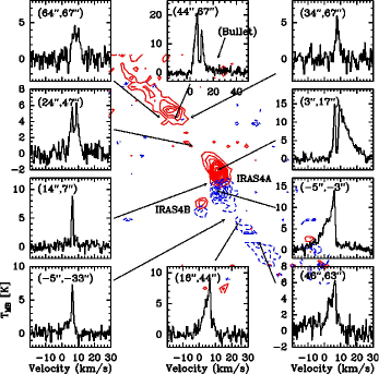
Figure 1: Gallery of ¹²CO 6–5 spectra from 10 different locations. Spectra of the IRAS 4A and 4B central positions are shown in Fig. 2. The arrows indicate the exact locations of the corresponding spectra with respect to the outflow lobes and each spectrum is given with the offset from IRAS 4A. Note the mix of narrow ($<$2 km s^-1) and medium (10–15 km s^-1) profiles together with the broad lines (25–30 km s^-1) at the outflowing positions close to the center of IRAS 4A. Also note that the velocity scale of the (44$\arcsec$,67$\arcsec$) panel is different to emphasize the weak “bullet” emission (see text). The vertical scale is for $T_{\rm mb}$. The contours are ¹²CO 6–5 emission where the levels start from 3$\sigma$ (15 K km s^-1) with an increasing step size of 2$\sigma$ (10 K km s^-1). The blue and red velocity ranges are selected from -20 to 2.7 and from 10.5 to 30 km s^-1, respectively.

3.1 CO line gallery

Figure 1 illustrates the quality of the APEX spectra as well as the variation in line profiles across the map. Several different velocity components can be identified, which are best seen at the central source positions. Figure 2 presents the gallery of CO lines at IRAS 4A and 4B using the APEX, JCMT, Herschel, IRAM 30m, Onsala and FCRAO telescopes. Available spectra of ¹²CO, ¹³CO, C¹⁸O, C¹⁷O and [C i] ranging from 1–0 up to 10–9 are shown. Integrated intensities and peak temperatures are summarized in Table 11 which includes the rms of each spectrum after resampling all spectra to the same velocity resolution of 0.5 km s^-1. The $S/N$ and dynamic range in the spectra is generally excellent with peak temperatures ranging from 30 mK to $>$20 K compared with the rms values of 0.006 to 0.4 K. Note in particular the very high $S/N$ obtained at the C¹⁸O 5–4 line with Herschel ($\sim$6 mK in 0.5 km s^-1 bins). Even C¹⁸O appears detected up to $J$=10–9 in IRAS 4B, albeit only tentatively (1.5 $\sigma$) in the 10–9 line itself. Together with the IRAS 2A data of Yıldız et al. (2010), this is the first time that the complete CO ladder up to 10–9 is presented for low-mass protostars, not just for ¹²CO but also for the isotopologs, and with spectrally resolved data.

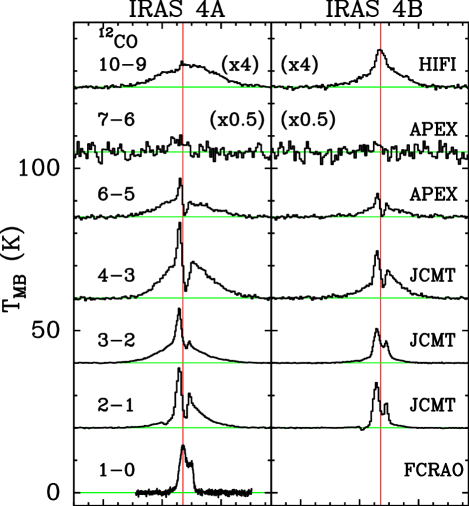
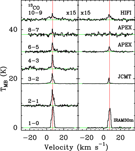
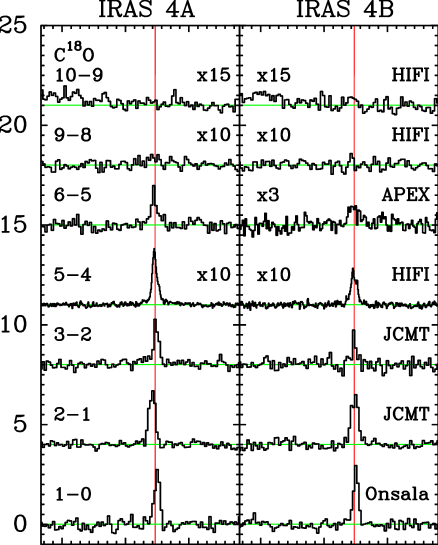
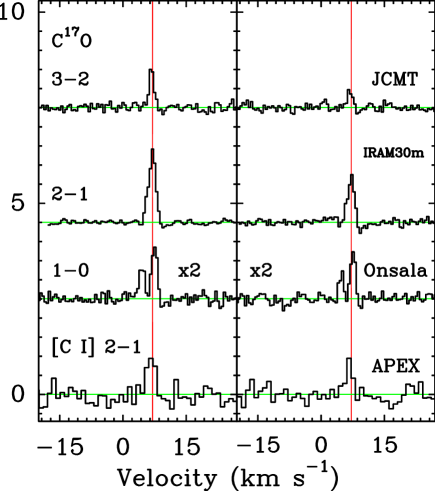
Figure 2: Single spectra obtained from the central positions of IRAS 4A and 4B presented on a $T_{\rm MB}$ scale. From bottom to top, Left: ¹³CO 1–0, ¹³CO 2–1, ¹³CO 3–2, ¹³CO 4–3, ¹³CO 6–5, ¹³CO 8–7, ¹³CO 10–9; ¹²CO 1–0, ¹²CO 2–1, ¹²CO 3–2, ¹²CO 4–3, ¹²CO 6–5, ¹²CO 7–6, ¹²CO 10–9; Right: [C i] 2–1, C¹⁷O 1–0, C¹⁷O 2–1, C¹⁷O 3–2; C¹⁸O 1–0, C¹⁸O 2–1, C¹⁸O 3–2, C¹⁸O 5–4, C¹⁸O 6–5, C¹⁸O 9–8, C¹⁸O 10–9. The spectra have been shifted vertically for viewing purposes and refer to the observing beams presented in Table 7. The red vertical line corresponds to the source velocity, $V_{\rm{LSR}}$, as measured from the C¹⁸O and C¹⁷O lines.

As discussed in Kristensen et al. (2010) based on H₂O spectra, the central line profiles can be decomposed into three components. A narrow profile with a FWHM of 2–3 km  s^-1 can mainly be found in the optically thin C¹⁸O and C¹⁷O isotologue lines at the source velocity. This profile traces the quiescent envelope material. Many ¹²CO and ¹³CO line profiles show a medium component with a FWHM of 5–10 km s^-1 indicative of small-scale shocks in the inner dense protostellar envelope ($<$1000 AU). The latter assignment is based largely on interferometry maps of this component toward IRAS 2A (Jørgensen et al. 2007). The ¹²CO lines are mainly dominated by the broad component with a FWHM 25–30 km s^-1 on $>$1000 AU scales representative of the swept-up outflow gas (Fig. 2).

Table 3: Observed line intensities for IRAS 4A and 4B in all observed transitions.

Source	Mol.	Transition	$\int T_{\rm MB}\mathrm{d}V$	$T_{\mathrm{peak}}$	Blue ($\int T_{\rm MB}\mathrm{d}V$)	Red ($\int T_{\rm MB}\mathrm{d}V$)	rms
			[K km s-1]	[K]	[K km s-1]	[K km s-1]	[K]
IRAS 4A	CO	1–0	60.1	13.0	1.1	26.1	0.45
		2–1	117.1	18.4	12.9	37.8	0.11
		3–2	128.0	16.8	34.4	30.6	0.07
		4–3	220.0	23.4	47.4	86.8	0.29
		6–5	110.5	11.9	31.8	37.4	0.33
		7–6	55.0	10.0	…	…	4.39
		10–9	40.7	1.9	9.9	17.6	0.07
	13CO	1–0	26.2	8.5	…	…	0.03
		2–1	16.0	6.5	…	…	0.23
		3–2	11.4	4.0	1.2	0.2	0.04
		4–3	15.2	5.7	…	…	0.36
		6–5	11.4	3.6	0.7	1.7	0.21
		8–7	2.4	2.2	…	…	0.39
		10–9	1.1	0.2	…	…	0.02
	C17O	1–0	1.8	0.7	…	…	0.05
		2–1	3.8	1.9	…	…	0.04
		3–2	1.6	1.0	…	…	0.09
	C18O	1–0	4.3	2.7	…	…	0.18
		2–1	4.9	2.7	…	…	0.13
		3–2	4.2	2.3	…	…	0.17
		5–4	0.6	0.4	…	…	0.006
		6–5	3.3	2.0	…	…	0.21
		9–8	0.16	0.05	…	…	0.02
		10–9	$<$0.05	…	…	…	0.02
	[C i]	2–1	2.3	1.0	…	…	0.21
I4A-B1	CO	3–2	92.8	14.0	64.8	10.1	0.37
		6–5	96.6	13.7	81.6	4.5	0.32
I4A-B2	CO	2–1	49.5	7.1	32.8	7.6	0.04
	13CO	2–1	11.6	3.7	…	…	0.03
I4A-B2	CO	3–2	71.2	12.3	12.8	40.5	0.42
		6–5	109.1	10.8	16.4	79.2	0.86
I4A-R2	CO	2–1	41.1	8.8	13.7	20.3	0.04
	13CO	2–1	13.3	4.6	…	…	0.03
IRAS 4B	CO	2–1	54.7	13.9	1.0	4.6	0.07
		3–2	57.0	10.5	6.6	6.7	0.05
		4–3	114.4	14.6	20.4	35.4	0.29
		6–5	52.3	5.9	10.7	16.5	0.34
		7–6	$<$39.0	…	…	…	4.51
		10–9	29.7	2.9	5.9	8.7	0.08
	13CO	1–0	23.9	7.9	…	…	0.09
		3–2	5.9	2.3	…	…	0.03
		6–5	6.8	2.0	0.4	0.8	0.16
		8–7	2.7	2.3	…	…	0.39
		10–9	0.6	0.15	…	…	0.02
	C17O	1–0	1.3	0.6	…	…	0.05
		2–1	2.3	1.3	…	…	0.06
		3–2	0.5	0.4	…	…	0.07
	C18O	1–0	4.4	2.9	…	…	0.18
		2–1	5.3	2.5	…	…	0.16
		3–2	1.9	1.7	…	…	0.23
		5–4	0.3	0.2	…	…	0.007
		6–5	0.9	0.4	…	…	0.07
		9–8	$<$0.06	…	…	…	0.02
		10–9	$<$0.06	…	…	…	0.02
	[C i]	2–1	1.8	0.9	…	…	0.17

3.2 Maps

The observations presented here are large scale $240^{\prime\prime}\times 240^{\prime\prime}$ maps in ¹²CO 6–5 and ¹²CO 3–2 covering the entire IRAS 4A/B region, together with smaller scale $80^{\prime\prime}\times 80^{\prime\prime}$ maps of ¹³CO 6–5 and [C i] 2–1 around the protostellar sources.

3.2.1 ¹²CO 6–5 map

The large ¹²CO 6–5 map over an area of 240$\arcsec\times$240$\arcsec$ ($\sim$56 500 $\times$ 56 500 AU) includes all the physical components of both protostars. Figure 3 (left) shows a ¹²CO 6–5 contour map of the blue and red outflow lobes, whereas Fig. 3 (right) includes the map of individual spectra overplotted on a contour map. This spectral map has been resampled to 10$\arcsec\times$10$\arcsec$ pixels for visual convenience, however the contours are calculated through the Nyquist sampling rate of 4$\arcsec$.5 $\times$ 4$\arcsec$.5 pixel size. All spectra are binned to 0.3 km s^-1 velocity resolution. The red and blue outflow contours are obtained by integrating the blue and red wings of each spectrum separately. The selected ranges are –20 to 2.7 km s^-1 for the blue and 10.5 to 30 km s^-1 for the red emission. These ranges are free of cloud and envelope emission and are determined by averaging spectra from outflow-free regions.

The ¹²CO 6–5 map shows a well-collimated outflow to the NE and SW directions centered at IRAS 4A with two knots on each side like a mirror image. Close to the protostar itself, the outflow appears to be directed in a pure N-S direction, with the position angle on the sky rotating by about 45$\degr$ at 10$\arcsec$ (2350 AU) distance. This N-S direction has been seen in interferometer data of Jørgensen et al. (2007) and Choi et al. (2011), and the high angular resolution of APEX-CHAMP⁺ now allows this component also to be revealed in single dish data. The morphology could be indicative of a rotating/wandering jet emanating from IRAS 4A or two flows from each of the binary components of IRAS4A. The outflow from IRAS 4B is much more spatially compact moving in the N-S direction. Overall, the CO 6–5 CHAMP⁺ maps are similar to the CO 3–2 map shown in Fig. 20 and in Blake et al. (1995). However, because of the $\sim$2 times larger beam, the N-S extension around IRAS 4A is not obvious in the 3–2 map and the knots are less ‘sharp’. Also, the compact IRAS 4B outflow is revealed clearly in single-dish data here for the first time. In the north-western part of the map, the southern tip of the SVS 13 flow is seen (HH 7–11; Curtis et al. 2010b).

3.2.2 ¹²CO 3–2 map

The large and fully sampled ¹²CO 3–2 JCMT HARP-B map covers the same area as the ¹²CO 6–5 map. In Fig. 20, the CO 3–2 contour and spectral maps presenting blue and red outflow lobes are shown. Here, the spectral map is resampled to 15$\arcsec\times$15$\arcsec$ pixels and the contours are calculated in the Nyquist sampling rate of 7.5″$\times$ 7.5″pixel size. The same velocity ranges as in the CO 6–5 map are used to calculate the blue and red outflow emission. Overall, the 3–2 map is very similar to those presented by Blake et al. (1995) and Curtis et al. (2010b).

The line ratio map of CO 3–2/CO 6–5 is presented in Fig. 4. The CO 6–5 map is convolved to the same beam as CO 3–2 and the peak antenna temperatures have been used to avoid having differences in line widths dominate the ratios. The distribution of the line ratios is flat at 0.8–1.0 around the center and outflow knots, with values up to 2.5 in the surrounding regions. As discussed further in Sect. 4.2.1, this implies higher temperatures towards the center and outflow knots than in the envelope at some distance away from the outflow.

Figure 5 shows maps of the maximum spectral velocities $V_{\rm max}$ obtained from the full width at zero intensity (FWZI) at each position for both the 6–5 and 3–2 maps. A 1.5$\sigma$ cutoff is applied in order to determine the FWZIs in both maps. Because of the lower rms of the data, CO 3–2 can trace higher velocities than CO 6–5. Overall, the profiles indicate narrow lines throughout the envelope with broad shocked profiles along the outflows (see also Fig. 1). Similar results have been found by van Kempen et al. (2009b) for the HH 46 protostar and outflow. The highest velocities with $V_{\rm max}=$25–30 km s^-1 are found at the source positions (where both red and blue wings contribute) and at the outflow knots.

Specifically, the IRAS 4A-R2 outflow knot has an extremely high velocity component (EHV or “bullet”) at $V\sim$ 20–35 km s^-1 as seen clearly in the 3–2 map (Fig. 21 in the Appendix). In the CO 6–5 map the “bullet” emission is only weakly detected ($\sim$5$\sigma$, Fig. 1) and is ignored in the rest of this paper.

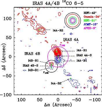
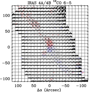
Figure 3: (Right:) ¹²CO 6–5 spectral map of IRAS 4A and 4B over the 240$\arcsec\times$240$\arcsec$ mapping area. Individual spectra are shown on the $T_{\rm MB}$ scale from –2 to 12 K and velocity scale from –20 to 30 km s^-1. The outflows of IRAS 4A and 4B are overplotted over the entire spectral map. The map is centered on IRAS 4A. The contour levels start from 3$\sigma$ (15 K km s^-1) with an increasing step size of 2$\sigma$ (10 K km s^-1). (Left:) Envelopes of IRAS 4A and 4B at the 10 K radius are shown together with the beam-sizes compared. See Fig. 1 caption and Sect. 3.2.1 for the details and the positions at which deep spectra are obtained.

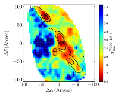
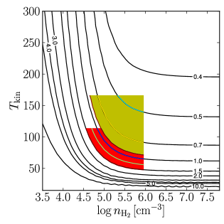
Figure 4: Left: Map of peak intensity ratios of the ¹²CO 3–2 /6–5 lines. Right: Model of the CO 3–2 / CO 6–5 line intensity ratio as function of temperature and density. The red region represents the observed range for IRAS 4A, the yellow range for IRAS 4B. CO column density is taken to be 10¹⁷ cm^-2 with a line width of 10 km s^-1, these conditions are chosen because they are representative of the observed CO 6–5 flux and line width. The coloured lines give the range of densities within the 20$\arcsec$ beam for the two sources based on the models of Kristensen et al. (subm). In the relevant density range, lower ratios imply higher temperatures.

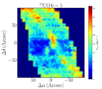
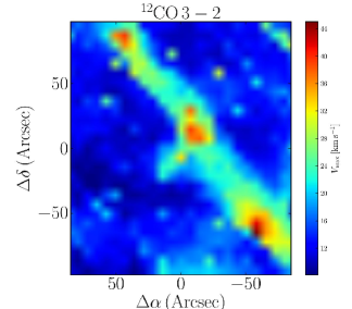
Figure 5: Maps of $V_{\rm max}$ obtained from full width at zero intensity (FWZI) at each position in both CO 6–5 (left) and CO 3–2 (right) maps.

3.2.3 ¹³CO 6–5 map

The ¹³CO 6–5 isotopolog emission was mapped over a smaller 80$\arcsec\leavevmode\nobreak\ \times$ 80$\arcsec$ region presented in Fig. 6. This map only covers the immediate environment of the protostellar envelopes of both protostars and the outflow of IRAS 4B. Figure 6 (left) shows the map of total integrated intensity whereas Fig. 6 (right) shows the spectral map with the outflow contours obtained using the same velocity range as in the CO 6–5 map. The ¹³CO 6–5 lines are not simple narrow gaussians, but show clearly the medium outflow component centered on the protostars. The medium component has a FWHM of $\Delta\varv$ = 8–10 km s^-1 while the narrow component is again $\Delta\varv$ = 1.5-2 km s^-1.

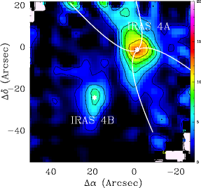
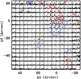
Figure 6: ¹³CO 6–5 maps of IRAS 4A (0,0) and IRAS 4B (22.5,-22.8). Left: Integrated intensity map of IRAS 4A and 4B in a 80$\arcsec\times$80$\arcsec$ area. The white elliptical biconical shape delineate the outflow cones as discussed in Sect. 6. Right: Blue and redshifted outflows seen in the ¹³CO 6-5 line profiles overplotted on a spectral map of the same region. Individual spectra are shown on a $T_{\rm MB}$ scale from –1 to 4 K and the velocity scale runs from –5 to 15 km s^-1. The contour levels for both figures are 3$\sigma$, 6$\sigma$, 9$\sigma$, … where $\sigma$=0.6 K.

3.2.4 [C i] 2–1 map

Figure 22 (in the Appendix) shows the weak detection of atomic carbon emission in and around the envelope and the outflow cavities, with the ¹²CO 6–5 red and blue contours overlaid (see also Fig. 3 right panel). This figure is the combination of three different observations, with one map covering only the central region (obtained in parallel with the ¹³CO 6–5 map). Thus, the noise level is higher at the edges of the figure. The spectra have been resampled to 1 km s^-1 velocity resolution in order to reduce the noise significantly; still, the [C i] line is barely detected with a peak temperature of at most 1 K. The weak emission indicates that CO is not substantially dissociated throughout the region, i.e., the UV field cannot contain many photons with wavelengths $<$1100 $\AA$ (van Dishoeck & Black 1988), as also concluded in van Kempen et al. (2009a). The low $S/N$ of the [C i] data precludes detection of any broad outflow component. Note that in HH 46, stronger [C i] emission is found at the bow shock position, but this line is still narrow ($\Delta V\sim$1 km s^-1; van Kempen et al. 2009b).

3.3 Morphology

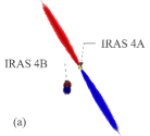
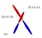
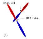
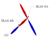
Figure 7: Four different projection scenarios of the IRAS 4A and 4B outflows are presented, assuming the two outflows have similar physical extents. These scenarios are treated by keeping the position of IRAS 4A fixed and rotating the plane of the sky $\sim$60$\degr$ for better comprehension the difference of IRAS 4B in (b)-(d). (a) shows the geometry as projected to the plane of the sky, (b) the protostars are at the same distance and very close to each other so that their envelopes overlap, (c) IRAS 4A is in front of IRAS 4B, (d) IRAS 4B is in front of IRAS 4A. In the latter two scenarios the envelopes may be sufficiently distant to each other and may not overlap.

By examining the morphology of the outflows from the CO 3–2 and 6–5 maps, it is possible to quantify the width and length of the outflows. The CO 6–5 map is used to calculate these quantities because of the two times higher spatial resolution. The length of the outflow, $R_{\rm CO}$, is defined as the total outflow extension assuming the outflows are fully covered in the map. By taking into account the distance to the source, the projected $R_{\rm CO}$ is measured as 105$\arcsec$ ($\sim$25 000 AU) and 150$\arcsec$ ($\sim$35 000 AU) for IRAS 4A for the blue and red outflow lobes, respectively. The difference in extent could be a result of denser gas deflecting or blocking the blue outflow lobe (Choi et al. 2011). For IRAS 4B, the extents are 12$\arcsec$ ($\sim$1 900 AU) and 9$\arcsec$ ($\sim$750 AU), respectively, but these should be regarded as upper limits since the IRAS 4B outflow is not resolved. The width of the IRAS 4A outflow is $\sim$20″($\sim$4 700 AU), after deconvolution with the beam size. These values do not include corrections for inclination.

The “collimation factor”, $R_{\rm coll}$ for quantifying the outflow bipolarity is basically defined as the ratio between the major and minor axes of the outflow. This quantity has been used to distinguish Stage 0 objects from the more evolved Stage I objects, in which the outflow angle has widened (Bachiller & Tafalla 1999; Arce & Sargent 2006). $R_{\rm coll}$ for IRAS 4A is found to be 5.3$\pm$0.5 for the blue outflow lobe and 7.5$\pm$0.5 for the red outflow lobe. For IRAS 4B, no collimation factor can be determined since the outflow is unresolved. Nevertheless, the much smaller extent of the IRAS 4B outflow raises the question whether IRAS 4B is much younger than IRAS 4A or whether this is simply an effect of inclination. The inclination of an outflow, which is defined as the angle between the outflow direction and the line of sight (Cabrit & Bertout 1990), can in principle be estimated from the morphology in the contour maps.

The IRAS 4 system is part of a clustered star-forming region so that the formation timescales for any of the YSOs in this region are expected to be similar. Also, the bolometric luminosities of IRAS 4A and 4B are comparable. For IRAS 4B, Herschel-PACS observations by Herczeg et al. (2011) detect only line emission from the blue outflow lobe, with the red outflow lobe hidden by $>$1000 mag of extinction. These new data support a close to face-on orientation with the blue lobe punching out of the cloud with little extinction and the red lobe buried deep inside the cloud. High resolution millimeter interferometer data of Jørgensen et al. (2007) as well as our data, however, do not show overlap between the IRAS 4B blue and red outflow lobes which would imply that they are not completely, but close to face-on with an inclination close to the line of sight of $\sim$15–30$\degr$. This range is consistent with 10–35$\degr$ suggested for IRAS 4B based on VLBI H₂O water maser observations (Desmurs et al. 2009). The large extent of the collimated outflow of IRAS 4A with, at the same time, high line-of-sight velocities suggests an inclination of $\sim$45–60$\degr$ to the line of sight. It is unlikely to be as high as 80–85$\degr$ as claimed for L1527 ($i$=85$\degr$) and L483 (80$\degr$; Tobin et al. 2008). Karska et al. (in prep.) find much lower velocities ($\sim$6–10 km s^-1) in CO 6–5 maps for these sources than in IRAS 4A/4B ($\sim$20–30 km s^-1).

Under the assumption that the intrinsic lengths of the flows are similar, Fig. 7 presents various options for the relative orientation of the two outflows viewed from different angles, all three of which can lead to the observed projected situation as seen in Fig. 7a. In the first scenario, the envelopes are very close to each other and interact accordingly (Fig. 7b). In the second scenario, the envelopes may be sufficiently separated in distance so that they do not interact with each other. In this case, IRAS 4A is either in front of IRAS 4B (Fig. 7c) or IRAS 4B is in front of IRAS 4A (7d).

The dynamical age of the outflows can be determined by $t_{\rm dyn}={R_{\rm CO}}/\overline{V}_{\rm max}$, where $\overline{V}_{\rm max}$ is the average total velocity extent as measured relative to the source velocity (Cabrit & Bertout 1992). $\overline{V}_{\rm max}$ for IRAS 4A and IRAS 4B are found to be $\sim$20 and $\sim$15 km s^-1, respectively, representative of the outflow tips (Fig. 5). Using these velocities, the $t_{\rm dyn}$ is 5900 and 9200 years for IRAS 4A for the blue and red outflow lobes, respectively. Knee & Sandell (2000) found 8900 yr (blue) and 16 000 yr (red) for the IRAS 4A outflow lobes, whereas Lefloch et al. (1998) found 11 000 years for both of the outflow lobes in IRAS 4A from an SiO 2–1 map. All these analyses assume a steady flow whereas the knots have clearly larger widths than the rest of the flow (Fig. 5), indicative of episodic accretion and outflow. Indeed, the constant flow assumption is the main uncertainty in the determination of dynamical ages, although our approach of taking the maximum velocity combined with the maximum extent should give more reliable estimates than ‘global’ methods (Downes & Cabrit 2007).

4 Analysis: Outflow

4.1 Rotational temperatures and CO ladder

The most direct quantity that can be derived from the CO lines at the source position are the rotational temperatures (Fig. 8). It is important to note that all lines are well fitted with a single temperature, indicating that they are probing the same gas up to $J$=10–9. Values of 69$\pm$7 and 83$\pm$10 K are found for ¹²CO, whereas those for ¹³CO and C¹⁸O are up to a factor of two lower (see Table 12). Since the ¹²CO integrated intensities are dominated by the line wings, this may indicate that the outflowing gas is somewhat warmer than the bulk of the envelope which dominates the isotopolog emission. On the other hand, the higher optical depths of the ¹²CO lines can also result in higher rotational temperatures. A quantitative analysis of the implied kinetic temperatures is given in Sect. 4.2.1.

Table 4: Rotational temperatures (in K) for the NGC 1333 sources

Source	12CO	13CO	C18O
IRAS 2A	61$\pm$8	…	34$\pm$4
IRAS 4A	69$\pm$7	38$\pm$4	25$\pm$4
IRAS 4B	83$\pm$10	29$\pm$3	26$\pm$4

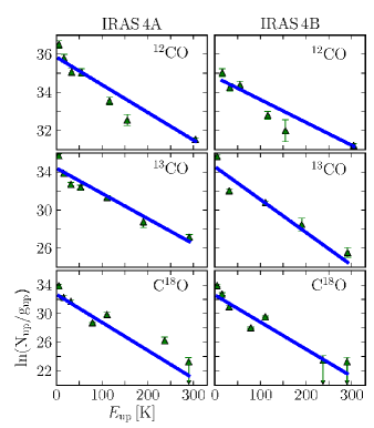
Figure 8: Rotation diagrams measured for the CO and isotopolog lines at the source positions of IRAS 4A and 4B. The column density of each observation in each rotational level divided by the statistical weight is plotted against the excitation energy of the level. The fitted line shows the Boltzmann distribution of the rotational populations. Derived values of the rotation temperatures are presented in Table 12.

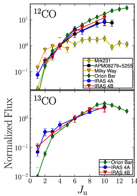
Figure 9: CO line fluxes for the observed transitions. The ¹²CO and ¹³CO lines are normalized relative to the $J$=4–3 and $J$=6–5 lines, respectively. Observations of the Milky Way (Wright et al. 1991), the dense Orion Bar PDR (Habart et al. 2010), the ultraluminous galaxy Mrk231 (van der Werf et al. 2010) and the high redshift quasar APM08279+5255 (Weiss et al. 2007a) are compared. In IRAS 4A and 4B, the available maps are convolved to 20$\arcsec$ in order to compare similar spatial regions.

Another way of representing the CO ladder is provided in Fig. 9 where ¹²CO and ¹³CO line fluxes are normalized relative to the $J$=4–3 and $J$=6–5 lines, respectively. Such figures have been used in large scale Milky Way and extragalactic studies to characterize the CO excitation (e.g. Weiss et al. 2007b). Other astronomical sources are overplotted for comparison, including the weighted average spectrum of diffuse gas in the Milky Way as measured by COBE-FIRAS from Wright et al. (1991); the dense Orion Bar PDR from Herschel-SPIRE spectra from Habart et al. (2010); SPIRE spectra of the ultraluminous infrared galaxy Mrk231 from van der Werf et al. (2010); and broad absoption line quasar observations of APM08279+5255 from ground-based data of Weiss et al. (2007a). For IRAS 4A and 4B, the ¹²CO and ¹³CO maps are convolved to 20$\arcsec$, where available, in order to compare similar spatial regions. It is seen that the low-mass YSOs studied here have very similar CO excitation up to $J_{u}=10$ to the Orion Bar PDR and even to ultraluminous galaxies; in contrast, the excitation of CO of the diffuse Milky Way and Mkr 231 appears to turn over at lower $J$. Our conclusion that the ¹³CO high-$J$ lines trace UV heated gas (§6) is consistent with its similar excitation to the Orion Bar.

4.2 Observed outflow parameters

The CO emission traces the envelope gas swept up by the outflow over its entire lifetime, and thus provides a picture of the overall outflow activity. The outflow properties can be derived by converting the CO line observations to physical parameters. Specifically, kinetic temperatures, column densities, outflow masses, outflow forces and kinetic luminosities can be derived from the molecular lines. In the following sections, the derivation of these parameters will be discussed.

4.2.1 Kinetic temperature

The gas kinetic temperature is obtained from CO line ratios. Figure 10 presents the observed line wing ratios of CO 3–2/6–5 at the source positions of IRAS 4A and 4B as well as the four outflow knots identified in Fig. 3. The CO 6-5 map is resampled to a 15$\arcsec$ beam so that the lines are compared for the same beam. The ratios are then analyzed using the RADEX non-LTE excitation and radiative transfer program (van der Tak et al. 2007), as shown in Fig. 4 (right). The density within the beam is taken from the modelling results of Kristensen et al. (subm) based on spherically symmetric envelope models assuming a power-law density structure (see Jørgensen et al. 2002, Sect. 5). The analysis assumes that the lines are close to optically thin, which is justified in Section 4.2.2. For the CO 6–5 transition, the critical density is $n_{\rm cr}$=1$\times$10⁵ cm^-3 whereas for CO 3–2, $n_{\rm cr}$=2$\times$10⁴ cm^-3 based on the collisional rate coefficients of Yang et al. (2010). For densities higher than $n_{\rm cr}$, the levels are close to being thermalized and are thus a clean temperature diagnostic; for lower densities the precise value of the density plays a role in the analysis.

From the adopted envelope model, the density inside $\sim$1750 AU (7.5$\arcsec$) is $>$10⁶ cm^-3 for both sources, i.e., well above the critical densities. The inferred temperatures from the CO 3–2/6–5 line wings are $T_{\rm kin}$ $\sim$60–90 and $\sim$90–150 K at the source centers of IRAS 4A and 4B. These values are somewhat lower than, but consistent with, the temperatures of 90–120 K and 140–180 K found in Yıldız et al. (2010) using the CO 6-5/10-9 line ratios. For the outflow positions B1 and R1, the density is $\sim$3$\times$10⁵ cm^-3 which results in temperatures of 100–150 K. The B2 and R2 positions are beyond the range of the envelope model, however assuming typical cloud densities of $\sim$10^4-5 cm^-3, the ratios indicate a higher temperature range of 140–200 K. Note that the line ratios in Fig. 10 are remarkably constant with velocity showing little to no evidence for a temperature change with velocity.

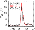
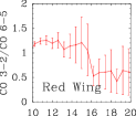
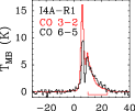
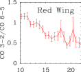
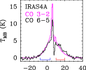
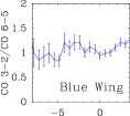
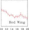
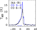
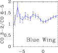
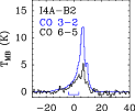
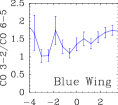
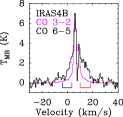
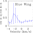
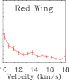
Figure 10: Ratio of the $T_{\rm MB}$ temperatures of ¹²CO 3–2/¹²CO 6–5. From top to bottom; left hand column shows IRAS 4A red outflow knots I4A-R2, I4A-R1, central source, blue outflow knots I4A-B1, I4A-B2 and IRAS 4B central source positions. Coordinates of these positions are given in Table 7. The spectra are binned to 0.6 km s^-1. The blue and red masks under the spectra in the left column show the range is used for the ratio calculations. Right hand column shows the ratios of these transitions.

4.2.2 Optical depths

The optical depth $\tau$ is obtained from the line ratio of two different isotopologs of the same transition. In Fig. 11, spectra of ¹²CO 6–5 and ¹³CO 6–5 at the IRAS 4A and 4B and ¹²CO 3–2 and ¹³CO 3–2 at the IRAS 4B source centers are shown. For presentation purposes, only the wing with the highest $S/N$ ratio is shown, but the same trend holds for the other wing. Figure 12 includes the spectra and line wing ratios of two dense outflow knots in ¹²CO 2–1 and ¹³CO 2–1 at positions labeled I4A-R2 (northern red outflow knot) and I4A-B2 (southern blue outflow knot). Line ratios are taken only from the line wings excluding the central narrow emission or self-absorption. The optical depths are then derived assuming that the two species have the same excitation temperature and the ¹³CO lines are optically thin. The abundance ratio of ¹²CO/¹³CO is taken as 65 (Langer & Penzias 1990). The resulting optical depths of ¹²CO as a function of velocity are shown on the right-hand axes of Figs. 11 and 12. High optical depths $>$2 are found at velocities which are very close to the central emission implying that the central velocities are optically thick and getting optically thinner away from the center in the line wings of the outflowing gas.

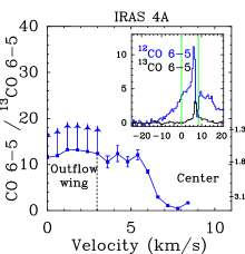
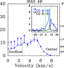
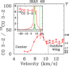
Figure 11: Ratio of $T_{\rm MB}$ ¹²CO 6–5/¹³CO 6–5 at the IRAS 4A and IRAS 4B source positions and ¹²CO 3–2/¹³CO 3–2 at the IRAS 4B in left, middle and right figures, respectively. The insets display the corresponding spectra and the green lines show the limits of the velocities over which these ratios are taken. The resulting optical depths of ¹²CO as a function of velocity are shown on the right-hand axes. The spectra are binned to 0.6 km s^-1.

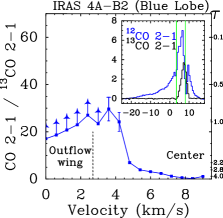
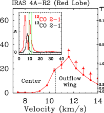
Figure 12: Ratio of $T_{\rm MB}$ ¹²CO 2–1/¹³CO 2–1 at the I4A-B2 (left) and I4A-R2 (right) outflow positions. The insets display the corresponding spectra and the green lines show the limits of the velocities over which these ratios are taken. The resulting optical depths of ¹²CO as a function of velocity are shown on the right-hand axes. The spectra are binned to 0.6 km s^-1.

4.2.3 Outflow Mass

The gas mass in a particular region can be calculated from the product of the column densities at each position and the surface area:

$$M_{\rm outflow}=\mu_{\mathrm{H_{2}}}\,m_{\rm H}\times\sum_{i}(N_{{\rm H_{2}},i}\times A)$$ (1)

where the factor $\mu_{\mathrm{H_{2}}}$=2.8 includes the contribution of Helium (Kauffmann et al. 2008), $m_{\rm H}$ is the mass of the hydrogen atom, $A$ is the surface area in one pixel (4$\aas@@fstack{\prime\prime}$5$\times$4$\aas@@fstack{\prime\prime}$5), $\sum_{i}N_{\rm H_{2},i}$ is the pixel averaged $\rm H_{2}$ column density over the selected velocity range, and the sum is over all pixels. In order to calculate the mass of the outflowing material, the CO 3–2 and 6–5 maps are resampled to a Nyquist sampling rate and calculated separately for each 15^′′ and 9^′′ pixel, respectively. As found in Sect. 4.2.2, the bulk of the emission in the line wings has low optical depth. The CO column density is then obtained from

$$\frac{N_{\rm u}}{g_{\rm u}}=\beta\frac{(\nu[\rm{GHz])^{2}}\,W[\mathrm{K\,km\,s^{-1}}]}{A_{\rm ul}[\rm s^{-1}]\,g_{\rm u}}$$ (2)

where $\beta$ = 1937 cm^-2; $g_{\rm u}$=2$J$+1 and $W=\int T_{\rm mb}{\rm d}V$ is the integrated intensity over the line wing. This intensity is calculated separately for the blue and red line wings with the velocity ranges as defined in Sect. 3.2.3. The total CO column density, $N_{\rm t}$, can then be found by

$$N_{\rm t}=N_{\rm u}Q_{\rm T}\frac{1}{g_{\rm u}\,e^{-E_{\rm u}/kT_{\rm ex}}}$$ (3)

where $Q_{\rm T}$ is the partition function corresponding to a specific excitation temperature, $T_{\rm ex}$. The assumed $T_{\rm ex}$ is 75 K based on Sect. 4.2.1, but using $T_{\rm ex}$=100 K results in only $\sim$10$\%$ less mass. The column density $N_{\rm H_{2}}$ is obtained assuming an ¹²CO/H₂ abundance ratio of $10^{-4}$ which is lower than the canonical value of 2.7$\times$10^-4 (Lacy et al. 1994). The precise value of the CO abundance in the outflow is uncertain because some of the CO may be frozen out onto dust grains. The total H₂ column densities in the outflows derived from the CO 6–5 data are 1.0 and 1.8$\times 10^{22}$ cm^-2 for IRAS 4A, and 1.0 and 0.9$\times 10^{21}$ cm^-2 for IRAS 4B, summed over the entire blue and red outflow lobes, respectively (see Table 13).

The masses of the outflowing material in the IRAS 4A blue and red lobes are then 6.1$\times 10^{-3}$ and 1.0$\times 10^{-2}$ M_⊙, and for IRAS 4B, 6.0$\times 10^{-4}$ and 5.3$\times 10^{-4}$ M_⊙, respectively. The masses have also been calculated from the CO 3–2 map, and the resulting values are $\sim$2 times larger, which is partly due to the fact that this line traces the colder gas with assumed $T_{\rm ex}$=50 K. Curtis et al. (2010b) used the JCMT CO 3–2 map of the entire Perseus molecular cloud to calculate the masses of the outflows from many sources in the region. They obtained around a factor of two higher mass for the total outflow in IRAS 4A (7.1$\times 10^{-2}$ vs. our measurement of 3.0$\times 10^{-2}$ $M_{\odot}$ from the 3–2 data) and around a factor of three higher value for IRAS 4B outflow (1.1$\times 10^{-2}$ vs. our measurement 1.8$\times 10^{-3}$ $M_{\odot}$). These differences are well within the expected uncertainties, i.e., caused by choosing slightly different velocity ranges.

Table 5: Outflow properties of the red and blue outflow lobes of IRAS 4A and IRAS 4B.

Outflow properties
Source	Trans.	Lobe	${V_{\rm max}}$	$R_{\rm CO}$	$t_{\rm{dyn}}$	$N_{\rm H_{2}}$	Moutflow	$\dot{M}$	$F_{\rm CO}$	$L_{\rm{kin}}$
			[km s-1]	[AU]	[yr]	[cm-2]	[M⊙]	[M⊙ yr-1]	[M⊙ yr-1km s-1]	[L⊙]
IRAS 4A	CO 3–2	Blue	22	2.8$\times 10^{4}$	5.9$\times 10^{3}$	8.6$\times 10^{21}$	1.3$\times 10^{-2}$	2.1$\times 10^{-6}$	5.0$\times 10^{-5}$	2.9$\times 10^{-4}$
		Red	18	3.9$\times 10^{4}$	1.0$\times 10^{4}$	1.2$\times 10^{22}$	1.8$\times 10^{-2}$	1.7$\times 10^{-6}$	3.9$\times 10^{-5}$	2.0$\times 10^{-4}$
	CO 6–5	Blue	20	2.5$\times 10^{4}$	5.9$\times 10^{3}$	1.0$\times 10^{22}$	6.1$\times 10^{-3}$	1.0$\times 10^{-6}$	3.1$\times 10^{-5}$	2.2$\times 10^{-4}$
		Red	18	3.5$\times 10^{4}$	9.2$\times 10^{3}$	1.8$\times 10^{22}$	1.0$\times 10^{-2}$	1.1$\times 10^{-6}$	3.7$\times 10^{-5}$	2.5$\times 10^{-4}$
IRAS 4B	CO 3–2	Blue	18	3.5$\times 10^{3}$	…	4.6$\times 10^{20}$	6.7$\times 10^{-4}$	…	1.9$\times 10^{-5}$	1.1$\times 10^{-4}$
		Red	15	4.7$\times 10^{3}$	…	7.5$\times 10^{20}$	1.1$\times 10^{-3}$	…	2.0$\times 10^{-5}$	9.7$\times 10^{-5}$
	CO 6–5	Blue	20	1.9$\times 10^{3}$	…	1.0$\times 10^{21}$	6.0$\times 10^{-4}$	…	3.4$\times 10^{-5}$	2.5$\times 10^{-4}$
		Red	12	7.5$\times 10^{2}$	…	9.1$\times 10^{20}$	5.3$\times 10^{-4}$	…	7.7$\times 10^{-5}$	4.5$\times 10^{-4}$

4.3 Outflow energetics

Theories of the origin of jets and winds and models of the ‘feedback’ of young stars on their surroundings require constraints on the characteristic force and energetics of the flow to infer the underlying physical processes. Specifically, the outflow force, kinetic luminosity and mass ouflow rate can be measured from our data. The outflow force is defined as

$$F_{\rm CO}=\frac{1}{R_{\rm CO}}\,\mu_{\mathrm{H_{2}}}\,m_{\rm H}\times\sum_{i}(N_{{\rm H_{2}},i}\times A\times\Delta V_{{\rm max},i}^{2}.)$$ (4)

So far, this parameter has been determined by using lower-$J$ lines for several young stellar objects (Cabrit & Bertout 1992; Bontemps et al. 1996; Hogerheijde et al. 1998; van Kempen et al. 2009b). The kinetic luminosity can be obtained from

$$L_{\rm{kin}}=\frac{1}{2R_{\rm CO}}\,\mu_{\mathrm{H_{2}}}\,m_{\rm H}\times\sum_{i}(N_{{\rm H_{2}},i}\times A\times\Delta V_{{\rm max},i}^{3})$$ (5)

and the mass outflow rate,

$$\dot{M}=\frac{M_{\rm outflow}}{t_{\rm{dyn}}}.$$ (6)

The outflow parameters derived from the observations are presented in Table 13. No corrections factors cf. Cabrit & Bertout (1990) have been applied.

5 Analysis: Envelope properties and CO abundance

5.1 Envelope model

In order to quantify the density and temperature structure of each envelope, the continuum emission is modelled using the 1D spherically symmetric dust radiative transfer code DUSTY (Ivezić & Elitzur 1997). The method follows closely that of Schöier et al. (2002) and Jørgensen et al. (2002, 2005a), discussed further in Kristensen et al. (subm). The inner boundary of the envelope is set to be where the dust temperature has dropped to 250 K ($=r_{\rm in}$). The density structure of the envelope is assumed to follow a power law with index $p$, i.e., $n\propto r^{-p}$, with $p$ being a free parameter. The other free parameters are the size of the envelope, $Y=r_{\rm out}/r_{\rm in}$ and the opacity at 100 $\mu$m, $\tau_{100}$. A grid of DUSTY models was run and compared to the SEDs as obtained from the literature and radial emission profiles at 450 $\mu$m and 850 $\mu$m (Di Francesco et al. 2008). The best-fit solutions were obtained using a $\chi^{2}$ method and are listed in Table 14, where also the derived physical parameters for the envelopes are listed.

A complication for the IRAS 4A/4B system is that they are so close to each other that their envelopes could overlap. Figs. 3 and 13 compare the envelopes at the 10 K radius together with the observed beam sizes. The model envelopes show that they start to overlap almost immediately from the central protostars if the two sources are at the same distance. In that case, the summed density of the two envelopes does not drop below 1.5$\times$10⁶ cm^-3 (Fig. 13, left). Another scenario discussed in Sect. 3.2.3 is that the two sources are sufficiently separated in distance so that they do not interact and therefore have separate envelopes (Fig. 7c and 7d). The density and temperature profiles as function of radius for such a scenario are shown in Fig. 13 (right). Since the overlap area is small even in the case that the sources are at exactly the same distance, the subsequent analysis is done adopting this latter scenario.

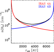
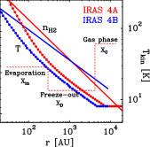
Figure 13: Power-law density profiles discussed for two scenarios in Section 4.3. In the left panel, the IRAS 4A position is taken as the reference and $r_{\rm AB}$ indicates the 4A-4B distance. In the right-hand panel the individual envelope profiles are shown. This panel includes a typical drop-abundance profile, with an outer abundance $X_{0}$, a freeze-out abundance $X_{D}$, and an inner abundance $X_{\rm in}$. In an anti-jump profile, the evaporation jump in the inner envelope is lacking.

Table 6: Spherical envelope models derived from dust continuum radiative transfer calculations of Kristensen et al. (subm).

Source	$Y$	$p$	$\tau_{100}$	$r_{\rm in}$	$r_{\rm out}$	$r_{\rm 10K}$	$n_{\rm r_{\rm in}}$	$n_{r_{\rm out}}$	$n_{\rm 10K}$	$N_{\rm H_{2},\rm 10K}$	$M_{\rm 10K}$
				[AU]	[AU]	[AU]	[cm-3]	[cm-3]	[cm-3]	[cm-2]	[$\mathrm{M_{\odot}}$]
IRAS 4A	1000	1.8	7.7	33.5	3.3$\times 10^{4}$	6.4$\times 10^{3}$	3.1$\times 10^{9}$	1.2$\times 10^{4}$	2.4$\times 10^{5}$	1.9$\times 10^{24}$	5.1
IRAS 4B	800	1.4	4.3	15.0	1.2$\times 10^{4}$	3.8$\times 10^{3}$	2.0$\times 10^{9}$	1.8$\times 10^{5}$	8.7$\times 10^{5}$	1.0$\times 10^{24}$	3.0

The resulting envelope structure is used as input for the Ratran line radiative transfer modeling code (Hogerheijde & van der Tak 2000). In Table 14, the inferred values from DUSTY that are used in Ratran are given. In IRAS 4A, the outer radius is taken to be the radius where the density $n$ drops to 1.2$\times$10⁴ cm^-3, and the temperature is considered to be constant after it reaches 8 K. The total masses of the envelopes are 5.1 M_⊙ (out to a radius of 6.4$\times$10³ AU) and 3.0 M_⊙ (3.8$\times$10³ AU) at the 10 K radius and 37.0 M_⊙ (3.3$\times$10⁴ AU) and 18.0 M_⊙ (1.2$\times$10⁴ AU) at the 8 K radius for IRAS 4A and 4B, respectively. The turbulent velocity is set to 0.8 km s^-1 which is representative of the observed C¹⁸O line widths. However, the narrow component of the ¹³CO lines is best fit with 0.5 and 0.6 km s^-1 for IRAS 4A and 4B, respectively. The model emission is convolved with the beam in which the line has been observed.

5.2 CO Abundance Profile

Yıldız et al. (2010) present Herschel-HIFI single pointing observations of CO and isotopologs up to 10–9 ($E_{\rm u}/k$=300 K) for NGC 1333 IRAS 4A, 4B and 2A. They used the C¹⁸O and C¹⁷O isotopolog data from 1–0 up to 9–8 to infer the abundance structure of CO through the envelope of the IRAS 2A protostellar envelope. For that source, the inclusion of the higher-$J$ lines demonstrates that CO must evaporate back into the gas phase in the inner envelope. In contrast, the low-$J$ lines trace primarily the freeze-out in the outer envelope (Jørgensen et al. 2002, 2005a). The maximum possible abundance of CO with respect to H₂ is 2.7$\times$10^-4 as measured in warm dense gas. Interestingly, the inner abundance in the warm gas was found to be less for IRAS 2A by a factor of a few. One goal of this study is to investigate whether this conclusion holds more commonly, in particular for the CO abundance profiles in IRAS 4A and 4B.

The CO abundance profile models were constructed for both IRAS 4A and 4B in the isotopolog lines of C¹⁸O and C¹⁷O using the methods outlined above. The lines are optically thin and have narrow line widths characteristic of the quiescent surrounding envelope. The CO-H₂ collision parameters from Yang et al. (2010) are used. The calibration errors are taken into account in the modelling. Following the recipe from Yıldız et al. (2010) for IRAS 2A, “constant”, “anti-jump”, “drop” and “jump” abundance profiles are investigated (see Fig. 13, right). The abundance ratio of C¹⁸O/C¹⁷O is taken as 3.65 (Wilson & Rood 1994).

5.2.1 Constant abundance profile

As a first iteration, a constant abundance was used to model the C¹⁸O and C¹⁷O lines, but it was not possible to reproduce all line intensities with this profile. In IRAS 4A, higher-$J$ C¹⁸O lines converge well around an abundance of $X$$\sim$6$\times$10^-8, however it is necessary to have lower abundances to produce lower-$J$ lines, around $X$$\sim$1–2$\times$10^-8. In IRAS 4B, higher-$J$ lines fit well $\sim$1$\times$10^-7 and lower-$J$ lines again with 1–2$\times$10^-8. Here, low-$J$ refers to the $J$ $\leq$3 lines and high-$J$ to the $J$ $\geq$5 lines.

5.2.2 Anti-jump abundance profile

For IRAS 4A, an anti-jump profile was run for the C¹⁸O and C¹⁷O lines. In an anti-jump profile, the evaporation jump in the inner envelope is lacking, that is, the inner abundance, $X_{\rm in}$=$X_{\rm D}$, and the depletion density, $n_{\rm de}$, are varied keeping the outer abundance high at $X_{0}$=5$\times$10^-7 corresponding to a ¹²CO abundance of 2.7$\times$10^-4 for ¹⁶O/¹⁸O=550 (see Yıldız et al. 2010, for motivation of keeping $X_{0}$ at this value). Reduced-$\chi^{2}$ plots are shown in Fig. 14 where lower and higher-$J$ lines are shown separately in order to illustrate their different constraints.

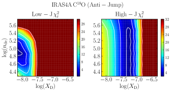
Figure 14: Reduced $\chi^{2}$ plots for the anti-jump abundance profile in IRAS 4A for the C¹⁸O lines in which the freeze-out abundance $X_{D}$ and depletion density $n_{\rm de}$ are varied. The left panel take the low-$J$ lines C¹⁸O 1–0, 2–1, 3–2 into account, whereas the right panels use the high-$J$ C¹⁸O 5–4, 6–5, 9–8 and 10–9 lines. The contours are plotted for the 1$\sigma$, 2$\sigma$, 3$\sigma$, 4$\sigma$, 5$\sigma$ confidence levels.

Lower-$J$ lines indicate an $n_{\rm de}$ of 7.5$\times$10⁴ cm^-3 and $X_{\rm D}$ of 1$\times$10^-8. The higher-$J$ lines do not constrain $n_{\rm de}$ but an upper limit of 2.5$\times$10⁵ cm^-3 and a well-determined $X_{\rm D}$ value of 5$\times$10^-8 are obtained. Because the density at the outer edge of the IRAS 4B envelope does not drop below 1.8$\times$10⁵ cm^-3, applying an anti-jump profile is not possible. CO remains frozen-out throughout the outer parts of the envelope.

5.2.3 Drop and Jump abundance profile

In order to fit all observed lines, a “drop” abundance profile is needed in which the inner abundance $X_{\rm in}$ increases above the ice evaporation temperature, $T_{\rm ev}$ (Jørgensen et al. 2005b), as was found for the IRAS 2A envelope (Yıldız et al. 2010). The $n_{\rm de}$ and $X_{\rm D}$ parameters inferred from the anti-jump profile from the low-$J$ lines are used to determine the evaporation temperature and inner abundance ($X_{\rm in}$). As for IRAS 2A, the reduced $\chi^{2}$ plots (not shown) indicate that the evaporation temperature is not well determined, thus a laboratory lower limit of $\sim$25 K is taken. Figure 15 left shows the $\chi^{2}$ plots in which the inner abundance $X_{\rm in}$ and $X_{\rm D}$ are varied. The models are run for a desorption density of 7.5$\times$10⁴ cm^-3 in IRAS 4A. Best fit values for the lower- and higher-$J$ lines are $X_{\rm in}\sim$1$\times$10^-7 and $X_{\rm D}$=5.5$\times$10^-8. For IRAS 4B, a jump abundance profile was applied in which the CO abundance stays low in the outer part (see Sect. 5.2.2). With this model, again, $X_{\rm in}$ and $X_{\rm D}$ values are varied (Fig. 15 right). The best fit gives $X_{\rm in}\leavevmode\nobreak\ \sim$3$\times$10^-7 and $X_{\rm D}$=1$\times$10^-8.

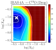
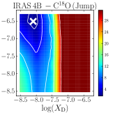
Figure 15: Reduced $\chi^{2}$ plots for the drop and jump abundance profile for the C¹⁸O lines in IRAS 4A and 4B, respectively. The freeze-out abundance $X_{\rm D}$ and inner abundance $X_{\rm in}$ are varied. All lines are taken into account except $J$=1–0 and 5–4 due to comparatively larger beam sizes. The contours are plotted at 1$\sigma$, 2$\sigma$, 3$\sigma$, 4$\sigma$ confidence levels and white crosses show the best-fit values.

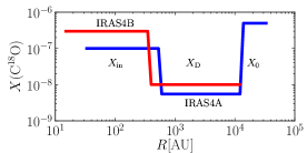
Figure 16: Schematic diagram showing the best-fit abundance profiles for IRAS 4A (blue) and IRAS 4B (red).

Best fit values obtained with the above mentioned models are summarized in Table 15 and a simple cartoon is shown in Fig. 16. Modeled lines are overplotted on the observed C¹⁸O lines in Fig. 17 convolving each line to the beam in which they have been observed. In the models, the C¹⁸O 1-0 and 5-4 lines are underproduced due to the fact that their much larger beam sizes pick up emission from the extended surroundings not included in the model.

Table 7: Summary of C¹⁸O abundance profiles for IRAS 4A and 4B.

Profile	$X_{\rm in}$	$T_{\rm ev}$	$X_{\rm D}$	$n_{\rm de}$	$X_{0}$
		[K]		[cm-3]
IRAS 4A
Constant	…	…	…	…	1–5$\times$10-8
Anti-jump	…	…	1$\times$ 10-8	7.5$\times$104	5$\times$10-7
Drop	$\sim$1$\times$10-7	25	5.5$\times$10-9	7.5$\times$104	5$\times$10-7
IRAS 4B
Constant	…	…	…	…	1-6$\times$10-8
Jump	3$\times$10-7	25	1$\times$ 10-8	…	1$\times$10-8
IRAS 2A
Constant	…	…	…	…	1.4$\times$10-7
Anti-jump	…	…	3$\times$ 10-8	7$\times$104	5$\times$10-7
Drop	1.5$\times$10-7	25	$\sim$ 4$\times$10-8	7$\times$104	5$\times$10-7

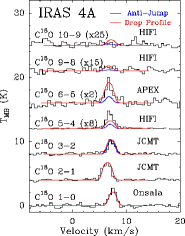
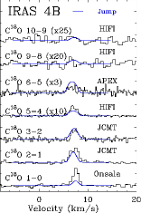
Figure 17: Left: Line profiles obtained with the best-fit anti-jump (blue) and drop abundance (red) envelope models overplotted on the observed C¹⁸O lines in IRAS 4A. Right: Similar best-fit jump abundance profile for IRAS 4B. See Table 15 for best-fit parameters.

Table 15 includes the IRAS 2A results from Yıldız et al. (2010). It is found that $X_{\rm in}$ is a factor of $\sim$3–5 lower than $X_{0}$ in IRAS 2A and a factor of 5 lower in IRAS 4A. Fuente et al. (2012) find a similar factor for the envelope of the intermediate mass protostar NGC 7129 IRS. Thus, the conclusion of Yıldız et al. (2010) for IRAS 2A that $X_{\rm in}<X_{0}$ holds more generally and is not linked to a specific source. This, in turn, may imply that a fraction of the CO is processed into other molecules in the cold phase when the CO is on the grains. The lack of strong centrally-peaked [C I] emission in the [C I] map indicates that CO is not significantly (photo)dissociated in the inner envelope.

6 Analysis: UV-heated gas

In addition to shocks, UV photons can also heat the gas. Qualitatively, the presence of UV-heated gas is demonstrated by the detection of extended narrow ¹²CO and ¹³CO 6–5 emission in our spectrally resolved data (Hogerheijde et al. 1998; van Kempen et al. 2009b; van Dishoeck et al. 2009). The fact that this emission is observed to surround the outflow walls (Sect. 3.2.1) suggests a scenario in which UV photons escape through the outflow cavities and either impact directly the envelope or are scattered into the envelope on scales of a few thousand AU (Spaans et al. 1995). Our map also shows narrow ¹²CO 6–5 emission at larger scales as well as in and around the bow-shock regions (Fig. 1). At these locations, the UV photons are most likely produced by the bow- and jet-shocks themselves, with the UV photons directly impacting the cavity walls and quiescent envelope. At velocities of 80 km s^-1 or more, these shocks produce photons with high enough energies that they can even photodissociate CO (Neufeld & Dalgarno 1989).

Quantitatively, the best constraints on the UV heated gas come from the narrow component of the ¹³CO emission. However, at the source positions, the passively-heated envelope also contributes to the intensity. To model this component, the best fitting C¹⁸O abundance profile for each source are taken and multiplied the abundance by the ¹³C/¹⁸O abundance ratio of 8.5. Figure 18 presents the resulting Ratran ¹³CO 6–5 line profiles at the central positions. The observed spectra for IRAS 4A and 4B are overplotted; here the (weak) broad component has been removed by fitting two gaussians to the spectra. The model spectra obtained with this profile are found to fit the ¹³CO 6–5 narrow emission profiles very well, implying that the contribution from the envelope is indeed significant.

In Fig. 19, the same method is applied to the entire ¹³CO 6–5 map to probe the extent of the envelope emission. In the middle panel, the observed integrated intensity map of only the narrow component is plotted. In the bottom panel, the ¹³CO map from the envelope model is convolved with the APEX beam and subsequently subtracted from the corresponding observed spectra. For both sources, the envelope model reproduces ¹³CO 6–5 emission at the central position. For IRAS 4B, no significant emission remains at off-source positions. For IRAS 4A, however, there is clearly narrow and extended emission visible beyond the envelope. Figure 19 top panel overplots the model envelope profiles on top of the observed profiles, showing that only the central positions are well reproduced by this model. The excess emission has a width of just a few km s^-1 so that it is not related to the outflow. Heating by UV photons is the only other plausible explanation. This interpretation is strengthened by the fact that the excess emission occurs precisely along the cavity walls, as shown in the bottom panel. The ¹³CO 6–5 transition requires a temperature of $T$$\approx$50 K to be excited which is consistent with model predictions of Visser et al. (2011) showing a plateau around this temperature on scales of a few 1000 AU from the protostar. Hence these observations constitute the first direct observational evidence for the presence of UV-heated cavity walls.

In order to compare the amount of gas heated by UV photons and gas swept up by the outflows, the masses in each of these components are calculated using the CO 6–5 and ¹³CO 6-5 data (narrow component only) over the same region. The mass of the UV-heated gas is calculated assuming $T_{\mathrm{ex}}$=75 K and CO/H₂=10^-4. Since the ¹³CO 6–5 map is smaller than that of CO 6–5, the outflow masses cannot simply be taken from Table 5, but are recomputed over the smaller area covered by the ¹³CO data. Both numbers are compared to the total gas mass in this area, obtained from the spherical model envelope based on the DUSTY results (see Sect. 5). To compare the same area as covered by the outflows, only the mass in an elliptical biconical shape is considered, with each cone taking $\sim$15% volume of the entire envelope out to the 10 K radius that would be present if the area had not been evacuated (see Fig. 6). The 10 K limit is still within the borders of the ¹³CO map (Fig. 3). The UV photon-heated gas mass is derived from the ¹³CO 6–5 narrow emission map where the envelope emission has been subtracted (bottom panel of Fig. 19). The inferred masses — total, UV-heated and outflow — are summarized in Table 16.

Interestingly, for IRAS 4A, the mass of UV-photon-heated gas is somewhat larger than that of the outflowing gas, demonstrating that UV photons can have at least an equally large impact on their surroundings as the outflows. Although the uncertainties in derived values are a factor of 2-3 (largely due to uncertainties in CO/H₂), both masses are only a few % of the total quiescent envelope mass in the same area, however. For IRAS 4B, UV photons are apparently unable to escape the immediate protostellar environment (see also discussion in Herczeg et al. 2011). In addition, the near pole-on geometry makes the detection of extended emission along the outflow cavity more difficult in this case.

Table 8: Comparison of photon-heated and outflow masses over the area mapped by ¹³CO 6–5.

Source	$M_{\rm total}$	$M_{\rm cones}$	$M_{\rm outflow}$	$M_{\rm UV}$
	Envelope	Envelope	12CO 6–5	13CO 6–5
IRAS 4A	5.0	1.5	3.7$\times 10^{-3}$	1.7$\times 10^{-2}$
IRAS 4B	3.1	0.9	1.0$\times 10^{-3}$	…

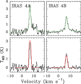
Figure 18: Top Panels: ¹³CO 6–5 spectra of IRAS 4A and 4B at the source positions. The green line is the fit to the narrow plus broad components. Bottom panels: The same lines after subtracting the broad component. The red line indicates the ¹³CO envelope model emission using the CO drop abundance profile derived from the C¹⁸O data. The figure indicates that a substantial fraction of the on-source emission comes from the passively-heated envelope. For IRAS 4A, however, there is also significant extended emission not due to the envelope (see Fig. 19).

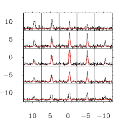
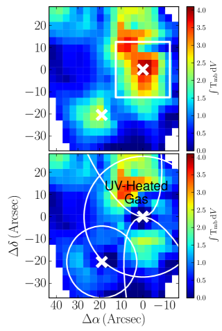
Figure 19: Top: Central region of the ¹³CO 6–5 map covering IRAS 4A. The broad component has been removed from the entire map. The red lines indicate the envelope model emission. Middle: Integrated intensity map of the narrow ¹³CO 6–5 emission, obtained by removing the broad component. The white square box indicates the region covered in the top figure. This map shows both the envelope and UV-heated gas. Bottom: ¹³CO map obtained after subtracting the model ¹³CO 6–5 envelope emission convolved to the APEX beam from the above map. White circles show the limits of the 10 K radius envelope and white cones show the direction of the outflows. This map represents the UV-heated gas only.

7 Conclusions

The two nearby Stage 0 low-mass YSOs, NGC1333 IRAS 4A and IRAS 4B, have been mapped in ¹²CO 6–5 using APEX-CHAMP⁺, with the map covering the large-scale molecular outflow from IRAS 4A. ¹²CO 6–5 emission is detected everywhere in the map. Velocity-resolved line profiles appear mainly in two categories: broad lines with $\Delta\varv>$10 km s^-1 and narrow lines with $\Delta\varv<$2 km s^-1. The broad lines originate in the molecular outflow whereas the narrow lines are interpreted as coming from UV heating of the gas. This interpretation is supported by the location of the narrow profiles: they “encapsulate” the broad outflow lines.

Comparing the CO 6–5 map with a CO 3–2 map obtained at the JCMT allows for a determination of the kinetic temperature in the outflow gas as a function of position through the outflow. The temperature peaks up at the outflow knots and exceeds 100 K. The temperature is found to be constant with velocity, and there is no indication of higher temperatures being reached at higher velocities. Our high $S/N$ multi-line data of ¹²CO and isotopologs have allowed us to derive excitation temperatures, line widths and optical depths, and thus the outflow properties, more accurately than before.

Smaller ¹³CO 6–5 maps centered on the source positions have also been obtained with APEX-CHAMP⁺. The ¹³CO 6–5 emission is detected within a 20″ radius of each source, and the line profiles are narrower than observed for the outflowing gas. The narrow ¹³CO emission traces gas with a temperature of $\sim$50 K at these densities, with the gas being heated by the UV photons. The mass of the outflowing gas is measured from the ¹²CO data, whereas the mass of the UV-heated gas is measured from the narrow ¹³CO spectra after subtracting the spherical envelope and outflow contributions. For IRAS 4A, the mass of the UV-heated gas is at least comparable to the mass of the outflow. This result shows that close to the source position on scales of a few thousand AU, UV heating is just as important as shock heating in terms of exciting CO to the $J$=6 level. Outflow- and envelope-subtracted ¹³CO 6–5 maps clearly reveal the first direct observational images of these UV-heated cavity walls.

Single-pointing C¹⁸O data have been obtained at the JCMT, APEX-CHAMP⁺ and most recently with Herschel-HIFI, the latter observing lines up to $J$=10–9. The data are used to constrain the CO abundance throughout the envelopes of the two sources. To reproduce the high-$J$ C¹⁸O emission, a “drop” in the abundance profile is required. This “drop” corresponds to the zone where CO is frozen out onto dust grains, and thus provides quantitative evidence for the physical characteristics of this zone. The CO abundance rises in the inner part where $T$ $>$ 25 K, but not to its expected canonical value of 2.7$\times$10^-4 (Lacy et al. 1994), indicating that some further processing of the molecule is taking place.

The combination of low-$J$ CO lines (up to $J$=3–2) and higher-$J$ CO lines such as $J$=6–5 opens up a new window for quantifying the warm ($T$ $\sim$100 K) gas surrounding protostars and along their outflows. These spectrally resolved data form an important complement to spectrally unresolved data of the same lines such as being observed of similar sources with Herschel-SPIRE. From our data it is clear that the ¹²CO lines covered by SPIRE are dominated by the entrained outflow gas with an excitation temperature of $\sim$100 K. For ¹³CO, lines centered on the protostar are dominated by emission from the warm envelope which is passively heated by the protostellar luminosity. Off source on scales of a few thousand AU, however, UV-photon heated gas along the cavity walls dominates the emission. The UV-heated component becomes visible in ¹²CO lines higher than 10–9, but it is likely that for Stage 0 sources this component will be overwhelmed by shocks for all lines in spectrally unresolved data (Visser et al. 2011). Thus, the ¹²CO and ¹³CO data provide complementary information on the physical processes in the protostellar environment: ¹²CO traces swept-up outflow (lower-$J$) and currently shocked (higher-$J$) gas, ¹³CO traces warm envelope and photon-heated gas. Our results imply that spectrally unresolved ¹²CO/¹³CO line ratios have only a limited meaning.

Understanding the excitation of chemically simple molecules such as CO is a prerequisite for interpreting other molecules, in particular H₂O data from Herschel-HIFI. Furthermore, understanding the distribution of warm CO on large spatial scales ($>$ 1000 AU) is necessary for interpreting future high spatial resolution data from ALMA.

Appendix A Auxillary Figures

We here present the CO 3-2 map obtained from JCMT, which is discussed in Sect. 3.2.2, and the CHAMP⁺ map of [C i] 2–1, which is discussed in Sect. 3.2.4.

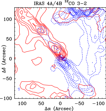
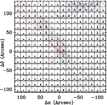
Figure 20: ¹²CO 3–2 spectral map of IRAS 4A and 4B over the 240$\arcsec\times$240$\arcsec$ mapping area. Individual spectra are shown on the $T_{\rm MB}$ scale from –2 to 16 K and velocity scale from –20 to 30 km s^-1. The maps are centered on IRAS 4A. The contour levels start from 20$\sigma$ (10 K km s^-1) with an increasing step size of 5 K km s^-1.

Figure 21: Blow-up of ¹²CO 3–2 spectra at the IRAS 4A-R2 outflow knot position. Bullet emission at +35 km s^-1 is visible in the upper left part of the IRAS 4A outflow. Individual spectra are shown on the $T_{\rm MB}$ scale from –0.7 to 2.5 K and velocity scale from –10 to 45 km s^-1. The coordinates are relative to IRAS 4A.

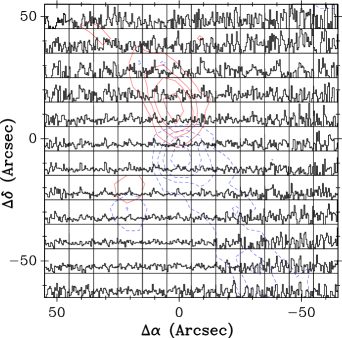
Figure 22: [C i] 2–1 spectral map (rebinned to 10$\arcsec$x10$\arcsec$ with a 1 km s^-1 velocity resolution) is overlaid on a ¹²CO 6–5 outflow contour map. In the [C i] 2–1 map, individual spectra are shown on a $T_{\rm MB}$ scale of –1 to 3 K and the velocity scale runs from –5 to 20 K km s^-1. The map is centered on the IRAS 4A position.