Resolving the Inner Structure of QSO Discs by Fold Caustic Crossing Events

Abstract

Though the bulk of the observed optical flux from the discs of intermediate-redshift lensed quasars is formed well outside the region of strong relativistic boosting and light-bending, relativistic effects have important influence on microlensing curves. The reason is in the divergent nature of amplification factors near fold caustics increasingly sensitive to small spatial size details. Higher-order disc images produced by strong light bending around the black hole may affect the amplification curves, making a contribution of up to several percent near maximum amplification. In accordance with theoretical predictions, some of the observed high-amplification events possess fine structure. Here we consider three putative caustic crossing events, one by SBS J1520+530 and two events for individual images of the Einstein’s cross (QSO J2237+0305). Using relativistic disc models allows to improve the fits, but the required inclinations are high, $i\gtrsim 70^{\circ}$. Such high inclinations apparently contradict the absence of any strong absorption that is likely to arise if a disc is observed edge-on through a dust torus. Still, the high inclinations are required only for the central parts of the disc, that allows the disc itself to be initially tilted by $60..90^{\circ}$ with respect to the black hole and aligned toward the black hole equatorial plane near the last stable orbit radius. For SBS J1520+530, an alternative explanation for the observed amplification curve is a superposition of two subsequent fold caustic crossings. While relativistic disc models favour black hole masses $\sim 10^{10}\mathrm{M_{\odot}}$ (several times higher than the virial estimates) or small Eddington ratios, this model is consistent with the observed distribution of galaxies over peculiar velocities only if the black hole mass is $\lesssim 3\times 10^{8}\mathrm{M_{\odot}}$.

1 Introduction

The history of gravitational lensing may be traced down to the beginning of the XXth century and beyond (see Schmidt & Wambsganss (2010) and references therein for a historical review). First double quasar images produced by strong lenses were reported in Walsh et al. (1979). The first quadruply-lensed quasar, QSO J2237+0305, was discovered by Huchra et al. (1985). This object was also the first were effects of microlensing by the stars of the lensing galaxy were found (Irwin et al., 1989).

The principal difference between strong lensing and microlensing is in the angular distance scale set by the Einstein-Chwolson radius:

$$\theta_{Ein}=\sqrt{\frac{4GM}{c^{2}}\frac{D_{LS}}{D_{S}D_{L}}}\simeq 2.8\ \sqrt{\frac{M}{\mathrm{M_{\odot}}}\frac{D_{LS}}{D_{L}}\frac{1\mathrm{Gpc}}{D_{S}}}\rm\mu as$$ (1)

Here, $M$ is the mass of the lensing object, $D_{L,S,LS}$ are angular size distances toward the lens (“L”), the source (“S”) and between the source and the lens (“LS”), $D_{LS}=D_{S}-D_{L}\times(1+z_{L})/(1+z_{S})$ for a flat Universe (see for example Hogg (1999)). Dependence on the lens mass leads to drastically different angular scales associated with strong lensing by galaxies and galaxy groups (arcseconds) and microlensing by individual stars (microarcseconds and less). The individual images formed in the latter case cannot be resolved by contemporary instrumentation, but their amplification variations may be a valuable tool to resolve the spatial structure of the source (Chang & Refsdal, 1984). Accretion discs around supermassive black holes at cosmological distances should have comparable or somewhat smaller angular sizes at $\lambda\sim 2000\rm\AA$. Below we will use spatial sizes projected onto the picture plane at the distance of the source. They differ from the angular sizes by the dimensional factor of $D_{S}$:

$$r_{Ein}=\sqrt{\frac{4GM}{c^{2}}\frac{D_{LS}D_{S}}{D_{L}}}\simeq 4.3\times 10^{16}\ \sqrt{\frac{M}{\mathrm{M_{\odot}}}\frac{D_{LS}}{D_{L}}\frac{D_{S}}{1\mathrm{Gpc}}}\rm cm$$ (2)

The main difference between microlensing by stellar mass objects of our Galaxy and microlensing effects accompanying strong lensing of quasars is in the optical depth. Angular distances between individual lensing bodies in a galaxy scale with the distance $D$ as $\propto D^{-1}$, while Einstein-Chwolson radii decrease only as $\propto D^{-0.5}$. If we define the microlensing optical depth as the total solid angle of the Einstein circles of the stellar population of a unit solid angle of the lensing galaxy (cf. Nityananda & Ostriker (1984)), it may be written as:

$$\tau=\frac{4\pi G\Sigma}{c^{2}}\frac{D_{LS}D_{L}}{D_{S}}\simeq 0.06\frac{\Sigma}{100\mathrm{M_{\odot}}\mathrm{pc}^{-2}}\frac{D_{LS}}{D_{S}}\frac{D_{L}}{1\mathrm{Gpc}}$$ (3)

Here, $\Sigma$ is the total surface density of the clumped matter in the lensing galaxy. Smoothly distributed component (primarily, unclumped dark matter) contributes only to strong lensing, unless it creates a strong shear that destroys point-lens degeneracy (Nityananda & Ostriker, 1984). Optical depth becomes considerably large ($\tau\gtrsim 0.1$) for lensed quasars at gigaparsec distances.

Difference in optical depth makes microlensing effects in distant lensing galaxies qualitatively different from the rare single- and double-lens events in our Galaxy. As a background source moves with respect to a single point-like lens, it has zero probability to undergo infinite amplification (Paczynski, 1986b). In this regime, amplification becomes sensitive to the size and the structure of the object only if its angular distance from the lens centre becomes comparably small. On the other hand, strong ($\tau\gtrsim 0.1..0.5$, depending on the underlying shear) microlensing by a population of point masses creates a network of fold caustics (Paczynski, 1986a) where amplification is divergent and behaves as $\propto d^{-1/2}$, where $d$ is the angular distance toward the fold (Chang & Refsdal, 1984). In the case of quasar microlensing, every particular image traverses some fold caustic at a probability of about unity on a several years’ time scale (for the case of QSO J2237+0305, the relative frequency of high-amplification events was estimated as $\sim 1\rm yr^{-1}$ by Witt et al. (1993), other objects have smaller relative proper motions). A comprehensive review on microlensing was made by Wambsganss (2006).

At present, there are at least three different approaches to quasar microlensing that may be used to probe the structure of supermassive black hole accretion discs. First is to gather statistics on image amplification and to compare single-epoch anomalous fluxes with the predictions of accretion disc models, as it was done by Pooley et al. (2007); Bate et al. (2008); Floyd et al. (2009); Blackburne et al. (2011); Jimenez-Vicente et al. (2012). In the first paper, a huge, about a factor of $10..100$, inconsistency was found between the sizes of accretion discs estimated by microlensing methods and predictions of the standard accretion disc theory. Partially, this inconsistency may be attributed to the crude mass estimates applying broad-band magnitudes with some assumptions on bolometric correction and accretion efficiency. On the other hand, Morgan et al. (2010) use more accurate mass estimates based on the widths of broad emission lines and yield much better consistency. Indeed, among the four objects common for the samples used in these two studies, only for one (QSO J2237+0305) the masses determined by the two methods are consistent within the uncertainties. For two objects (PG 1115+080 and RXJ 1131-1231), photometry-based mass estimates are about four times lower, while for the least massive one, SDSS 0924+0219, masses differ by an order of magnitude. However, the accretion disc sizes measured by Morgan et al. (2010) are still several times larger than expected. Authors suppose that virial mass estimates may still be systematically lower by a factor of $\sim 3$.

The analysis method used by Morgan et al. (2010) was introduced by Kochanek (2004) and may be characterised as extensive light curve fitting. A number of artificial amplification maps is generated, and the observational light curve is compared with numerous simulated light curves with random parameters. This technique was applied in a large number of studies such as Eigenbrod et al. (2008) and Hainline et al. (2012). Since the technique requires multiple observational points, it is perfect for Einstein’s cross and other targets of monitoring programmes.

The Monte Carlo microlensing analysis is rather resource-consuming. As an alternative to computationally-extensive methods, it is reasonable to study individual high-amplification events that are most sensitive to the spatial properties of the source. Primarily, high amplification events are associated to fold caustic crossings, when a pair of new microlensing images appears or disappears, and the point-source amplification diverges. Caustic crossings by standard discs are good models for some of the observed amplification events (Gil-Merino et al., 2006; Koptelova et al., 2007). It may be shown that point-source amplification during a caustic crossing is divergent for a disc with a small inner radius $r_{in}$ as $\mu\propto r_{in}^{-1/4}$, hence brightness maxima in microlensing curves are best fit for resolving the innermost parts of the disc (Agol & Krolik, 1999). Indeed, as it was shown by Jaroszynski et al. (1992), lensing curves differ for accretion discs of different inclinations and Kerr parameters of the accretor. Amplification curves primarily differ near their maxima.

Caustic crossing events allow to study the structure of the innermost parts of accretion discs where general relativity effects are important. Two processes are expected to influence considerably the observed light curves: light bending and Doppler boosting (due to matter motion in the disc as well as due to frame dragging). Both make brightness distributions asymmetric and strongly dependent on the inclination angle. In this paper we aim on estimating the influence of relativistic effects on the amplification curves created by straight caustic crossing events. We also apply the results of our calculations to three high amplification events and show that some of their features are probably connected to relativistic effects.

The paper is organized as follows: first we describe the archival observational data we use. Simulation technique applying Kerr geodesic calculation software is considered in section  3. Fitting results for the three putative caustic crossings are given in section  4 and discussed in section  5.

2 Observational Data

The current number of lensed quasars where microlensing effects were found is about several tens (Pooley et al., 2007; Morgan et al., 2010; Jimenez-Vicente et al., 2012). However, long homogeneous observational series exist for few objects. The best studied among these is the Einstein cross (QSO J2237+0305) that is a subject of extensive photometric monitoring programs such as OGLE-II (Woźniak et al., 2000) and -III (Udalski et al., 2006). We analyse two high-amplification events that took place for two different images in the years 1999 and 2000. We also found a considerable amount of archival data on another object, SBS J1520+530, and interpret variations of the relative image amplifications as a manifestation of microlensing amplification. A brief summary of the observational data we use in this work is given in table 1.

Table 1: Basic information about the objects and the observational amplification curves used for analysis. For the QSO J2237+0305 image A event, the numbers of GLITP data points for two reduction techniques, ISIS and PSF, are given separated by a slash.

	SBS J1520+530	QSO J2237+0305(A)	QSO J2237+0305(C)
source redshift	1.855	1.695
lens redshift	0.72	0.039
time span (V), JD-2450000		1400$..$1650	1200$..$1650
number of points (V)	–	53/52	83
time span (R), JD-2450000	1200$..$3000	1450$..$1510	–
number of points (R)	253	51/49	–

2.1 SBS J1520+530

The object is doubly imaged, with the average flux ratio for the two images A and B about 2 (Burud et al., 2002). The lens is a relatively distant ($z\simeq 0.7$) late-type elliptical with the estimated velocity dispersion of $\sigma\sim 200\mathrm{km\,s^{-1}}$, steep mass profile, central convergence of $\kappa\simeq 0.5$ and possible signatures of interaction with its environment (Auger et al., 2008). B is about three times closer to the lens centre, hence we expect moderate microlensing optical depth for B and small ($\tau\lesssim 0.1$) for A. Hence we are inclined to interpret the observed flux ratio variations as microlensing of the B image.

We used the three following sources of reduced photometric data (R-band magnitudes for both images) covering a time span of about seven years (see figure 1):

• 58 data points obtained with the Nordic Optical Telescope (NOT) and published by Burud et al. (2002)

• 60 observations with the 1.5-m Russian-Turkish Telescope RTT (Khamitov et al., 2006), kindly provided by I. Bikmaev and I. Khamitov

• 123 observations with the 1.5m AZT-22 telescope in Maidanak. These data were described, analysed and published by Gaynullina et al. (2005).

All the photometry was performed in the standard optical R band that for the source redshift of $1.855$ (Barkhouse & Hall, 2001) corresponds to $\lambda\simeq 2000..2500\rm\AA$ in the source reference frame.

Figure 1: R-band light curves for A (upper panel) and B (lower panel) images of SBS J1520+530. Filled circles, asterisks and diamonds represent NOT, RTT and Maidanak data (see text, section 2.1).

Relatively large amount of data allows to improve the estimate of delay time. Cross-correlating the time series for the two images we find a broad peak at $\Delta t=127.6\pm 2.0$ days that we interpret as the delay between the two images. Within the uncertainties (that are hereafter calculated for 90% significance level), this value is consistent with the 130$\pm$3 day delay found by Burud et al. (2002) and Gaynullina et al. (2005) and with the 128-day estimate by Khamitov et al. (2006). This value of $\Delta t$ is subsequently used to shift the series of A and B fluxes and estimate flux ratios.

Merged time series consists of 241 unevenly-sampled R-band observational points for each image (see figure 1). To minimize information losses but to avoid unjustified interpolation (on periods of time longer than tens of days), we construct flux ratios by linearly interpolating the magnitudes between the observational points. The resulting flux ratio series consists of points of two kinds: $(i)$ B image fluxes shifted backwards by $\Delta t$ and divided by the interpolated values of A image flux and $(ii)$ interpolated B image fluxes divided by the A image fluxes shifted forward by $\Delta t$. We did not interpolate over time gaps longer than 45d (about 16d in the frame co-moving with the object), therefore the resulting time series contains only 360 points, not entirely independent (see also section 4.1).

Figure 2: Ratios of delay-corrected fluxes of images A and B of the lensed QSO SBS J1520+530. Thin horizontal line is the mean ratio value, thick horizontal line with ticks marks the time span used for our analysis.

Flux ratio curve (see figure 2) demonstrates a maximum at the Julian date $JD\sim 2451500$ and another one at $JD\sim 2451800$, that form together an about two-year long structure similar to standard disc amplification curves (see next section). For the remaining two-thirds of the curve, $B/A$ ratio is stable and close to 0.47 with standard deviation around four percent. From the resulting time series, we excluded the final portion of the curve between $JD=2453000..2453600$ where the data are sparse and the observed variability is difficult to relate to the high-amplification event in the earlier part of the data (see figure 10). The resulting amplification curve consists of 253 data points.

2.2 QSO J2237+0305

We use R- and V-band photometric data on the images A and C of QSO J2237+0305. The data were taken from two sources:

• OGLE-II Huchra’s lens monitoring program (Woźniak et al., 2000), the data are available at http://ogle.astrouw.edu.pl/cont/4_main/len/huchra/huchra_ogle2.html and contain V-band magnitudes for the four images

• GLITP archive (Alcalde et al., 2002): V- and R-band magnitudes for all the images, reduced data are available at http://wela.astro.ulg.ac.be/themes/extragal/gravlens/bibdat/engl/lc_2237.html.

The light curves are shown in figure 3. The data sample is similar to that used by Koptelova et al. (2007). We use GLITP data reduced by two different techniques: ISIS photometry (the magnitudes are available at the web page given above) and PSF-fitting (the magnitudes are meant to be available for download but the link is broken, hence we asked Elena Shimanovskaya who has kindly provided us with these magnitudes). The two reduction techniques are compared in Alcalde et al. (2002). Magnitudes reduced by different techniques are generally consistent but deviate considerably (by about $0.\!^{\rm m}03$) near the maximum of the image A high-amplification event. Unfortunately, the maximum interferes with a period of bad visibility of the object (January/February 2000). OGLE points show unreasonably large scatter near JD=2451500. Besides, consistency between OGLE and GLITP data during this period is poor and insufficient for our purposes (see figure 3, left panel). Better but still significant deviations between the GLITP magnitudes reduced with different methods (we show only ISIS-reduced data to prevent the figure from overcrowding; the two GLITP light curves are shown together in figure 12). Therefore we exclude OGLE data from subsequent analysis for the image A event.

GLITP data during the maximum of image A brightness demonstrate a double-peaked structure that we are inclined to interpret as a signature of the inner disc structure. Overall behaviour near Julian dates 2451520$..$2451540 suggests that the dip is real and has an amplitude of about 0$.\!^{\rm m}$02.

For the C image event, most of GLITP observational points are far away from the high amplification event maximum, and we finally fit only the V-band OGLE data.

Figure 3: Raw light curves of the images A (left) and C (right) of QSO J2237+0305 used in the current work. GLITP(ISIS) data are shown by filled circles, OGLE data points by asterisks. Date intervals used for fitting are restricted by vertical lines.

There is strong evidence that the individual time delays for the images of QSO J2237+0305 are very small, such as several days (see Koptelova et al. (2006) and references therein). We can make use of the relative proximity of the lens that makes the microlensing variability of individual images much faster and stronger than the intrinsic variability of the source. The studied high amplification events last less than a year, and variability of individual images does not show any detectable correlation on these time scales. Einstein cross is known for its lack of variability, the maximal gradients of intrinsic variability are considerably smaller than microlensing trends (see for example Eigenbrod et al. (2008)).

3 Amplification curve simulation technique

3.1 Basic assumptions

All the three high-amplification events are good candidates for caustic crossings. We model them by convolving a straight caustic crossing curve with a standard disc profile integrated over one dimension. Simplified flat and non-relativistic (section 3.2) and general relativistic (section 3.3) disc models were used. In both cases we consider a multi-blackbody disc with monochromatic intensity obeying the Planck law with the temperature determined by the standard accretion disc model:

$$\begin{array}[]{l}I\propto\frac{1}{\exp\left(\frac{h\nu}{T(r)}\right)-1}=\\ \qquad{}=\frac{1}{\exp\left(\left(r/r_{d}\right)^{3/4}\left(1-\sqrt{r_{in}/r}\right)^{1/4}\right)-1},\\ \end{array}$$ (4)

where r is the radial coordinate, and $r_{d}$ and $r_{in}$ are, correspondingly, the radial scale of the disc and its innermost stable orbit radius defined as:

$$r_{d}=\left(\frac{k}{hc}\frac{\lambda}{1+z}\right)^{4/3}\left(\frac{3}{2}\frac{l}{\eta}\frac{G^{2}M^{2}}{c\sigma\kappa}\right)^{1/3}$$ (5)

$$r_{in}=x_{\rm ISCO}(a)\frac{GM}{c^{2}}$$ (6)

Here, $k$, $\sigma$ and $h$ are Boltzmann, Stephan-Boltzmann and Planck constants, $c$ is the speed of light, $l$ and $\eta$ are Eddington ratio and overall accretion efficiency, $\varkappa$ is Thomson opacity, $\varkappa\simeq 0.35\rm cm^{2}\,g^{-1}$ for Solar composition. Dimensionless innermost stable circular orbit radius $x_{\rm ISCO}(a)$, as well as efficiency $\eta=\eta(a)$, may be found analytically as functions of dimensionless Kerr parameter $a$ (Bardeen et al., 1972).

Expression (4) was derived for monochromatic intensity (no matter $I_{\nu}$ or $I_{\lambda}$) but is to a high accuracy valid even for broad-band photometry if most of the radiation comes in the form of a smooth continuum. Mean effective wavelength varies by less than 2% for the spectral slope varying from $p=-1$ to $p=1$, where $F_{\nu}\propto\nu^{p}$. The above definition of $r_{d}$ is identical to the characteristic radius used by Morgan et al. (2010). Note however that it is generally sufficiently smaller (by a factor of $\sim 2.44$ for a standard disc with no inner edge) than the half-light radius. We will see below that for the shape of amplification curve, the quantity of principal importance is the ratio of the two radial scales given by (5) and (6):

$$\begin{array}[]{l}X=\frac{r_{d}}{r_{in}}=\\ \qquad{}=\left(\frac{k}{h}\frac{\lambda}{1+z}\right)^{4/3}\left(\frac{3}{2}\frac{l}{\eta(a)}\frac{c}{GM\sigma\varkappa_{T}}\right)^{1/3}\simeq\\ \simeq 92\left(\frac{\lambda/1\mu}{1+z}\right)^{4/3}\left(\frac{l}{0.25}\right)^{1/3}\left(\frac{\eta(a)}{0.1}\right)^{-1/3}\left(\frac{M}{10^{9}\mathrm{M_{\odot}}}\right)^{-1/3}x_{ISCO}^{-1}(a)\\ \end{array}$$ (7)

For fixed $X$, the differences between amplification curves are important only for high inclinations and are connected to relativistic effects, namely Doppler boosting and light bending. Variations of the Kerr parameter may change $X$ by a factor of $\max(x_{ISCO})/\min(x_{ISCO})=9$. Inversely, one may reasonably estimate $X$ by fitting the amplification curve and arrive to a tightly correlated pair of uncertain $a$ and $M$. Having reasonable mass estimates, one may thus make an estimate for $a$, and vice versa.

Below, we fix the Eddington ratio to $l=0.25$. The black hole masses are estimated as $M=8.8\times 10^{8}\mathrm{M_{\odot}}$ for SBS J1520+530 and $M=9\times 10^{8}\mathrm{M_{\odot}}$ for QSO J2237+0305 by Morgan et al. (2010). These mass estimates were obtained using emission line profiles (see references given by Morgan et al. (2010)) and virial relations (Vestergaard & Peterson, 2006). Accuracy of these estimates is low, about 0.3dex. Our analysis yields generally higher masses poorly consistent with the virial estimates (see below section 4). In fitting the observational data, we first find $X$, inclination $i$ and positional angle $\psi$ and then optimize for the mass and Kerr parameter, fixing $X$.

Caustic is considered a straight line defined by condition $y=v_{eff}\times(t-t_{0})$ at the given time $t$. Let $x$ and $y$ be the coordinates in the picture frame along and across the caustic, respectively. The origin of this coordinate system coincides with the black hole centre. In the general case, the disc is inclined, and it is convenient to use the coordinate system $(\alpha,\beta)$ defined by the major and the minor axes of the disc projection upon the picture frame (as in Dexter & Agol (2009)). The two coordinate systems in the picture frame are connected by rotation by an angle of $\psi$ that has the meaning of relative positional angle of the normal to the disc with respect to the normal to the caustic (see a sketch in figure 4). Without any loss of generality we assume that the relative motion of the source and lens is normal to the caustic itself. Integration over one direction is convenient to consider as projection upon the orthogonal direction.

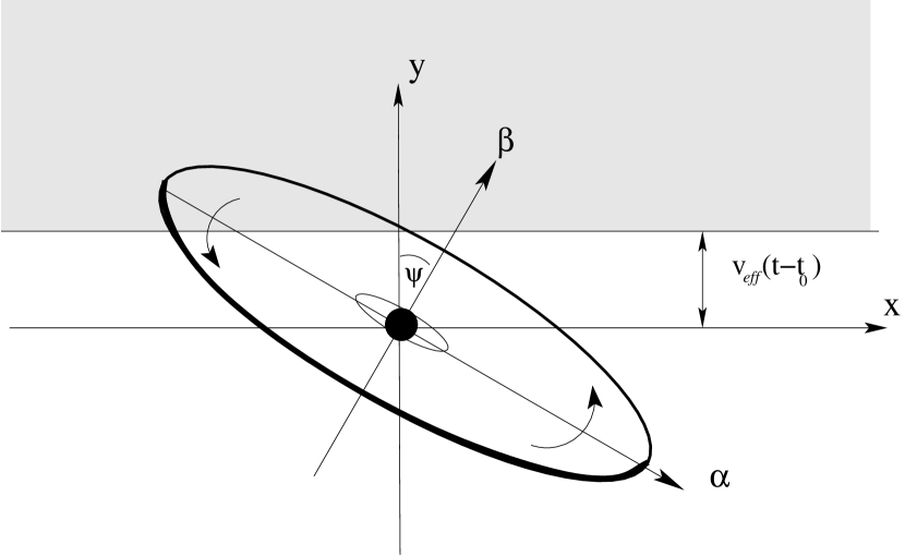
Figure 4: A qualitative scheme showing the two coordinate systems in the picture plane. Shaded is the area behind the caustic where amplification is higher. Disc is inclined with respect to the observer, and its closer side is shown by a thicker curve.

Effective velocity $v_{eff}$ is calculated as the relative proper motion multiplied by the angular size distance $D_{S}$ toward the object. Our analysis is sensitive only to its component perpendicular to the caustic direction. The velocity is connected to the peculiar spatial velocities of the QSO ($\mathbf{v_{S}}$) and the lensing galaxy ($\mathbf{v_{L}}$) in the following way:

$$v_{eff}=\frac{\mathbf{v}_{S}\cdot\mathbf{n}}{1+z_{S}}-\frac{\mathbf{v}_{L}\cdot\mathbf{n}}{1+z_{L}}\frac{D_{S}}{D_{L}}+\frac{\mathbf{v}_{o}\cdot\mathbf{n}}{1+z_{L}}\frac{D_{LS}}{D_{L}}$$ (8)

Third term describes the peculiar motion of the observer, $v_{o}\sim 370\mathrm{km\,s^{-1}}$ is known from the dipole constituent of cosmological CMB variations (see for example Lineweaver et al. (1996)). Unit vector $\mathbf{n}$ is normal to the caustic and lies in the picture plane. Reasonable limit for peculiar motion velocities of individual galaxies is $v\lesssim v_{max}\simeq 2000\mathrm{km\,s^{-1}}$ that corresponds to about $2..3$ rms values for the radial peculiar velocity distribution (Raychaudhury & Saslaw, 1996). This limit may be converted to the condition for the possible effective transverse velocity $v_{eff}\lesssim v_{max}\sqrt{(1+z_{S})^{-2}+(1+z_{L})^{-2}\times(D_{S}/D_{L})^{2}}$. For SBS J1520+530, $\mathbf{v_{S}}$ and $\mathbf{v_{L}}$ contributions are of the same order because $D_{S}/D_{L}\simeq 1.2$. In this case, $v_{eff}\lesssim 1600\mathrm{km\,s^{-1}}$. For QSO J2237+0305, the lens is about ten times closer ($D_{S}/D_{L}\simeq 11$) and $v_{eff}\lesssim 20\,000\mathrm{km\,s^{-1}}$.

3.2 Simplified standard disc

Besides the more sophisticated model described below, we use a simple disc approximation ignoring all relativistic effects. In this approximation and for the straight caustic case, inclination does not affect the observed shape of the amplification curve. This is valid for a thin disc of arbitrary inclination as long as the disc is thin enough ($h/R\ll\cos i$, where $i$ is inclination).

We are interested in intensities integrated over one dimension. Here, we provide the general form for the integral over one direction (we make a substitute $t=x/y$):

$$\begin{array}[]{l}I_{1}(y)=\int I(x,y)dx\propto\\ \qquad{}\propto\sqrt{\frac{J}{K}}y\int_{t_{in}}^{+\infty}\frac{dt}{\exp\left(\left(\frac{y^{2}}{r_{d}^{2}}J\times(1+t^{2})\right)^{3/8}f^{-1/4}\right)-1},\end{array}$$ (9)

where:

$$K=K(i,\psi)=\cos^{2}\psi+\frac{\sin^{2}\psi}{\cos^{2}i},$$ (10)

$$J=J(i,\psi)=\sin^{2}\psi+\frac{\cos^{2}\psi}{\cos^{2}i}-\frac{\sin^{2}\psi\cos^{2}\psi}{K(i,\psi)}\tan^{4}i,$$ (11)

$$f=1-\left(\frac{1}{J}\frac{r_{in}^{2}}{y^{2}}\frac{1}{1+t^{2}}\right)^{1/4}$$ (12)

$$t_{in}=\left\{\begin{array}[]{lc}0&\mbox{ if }y\geq r_{in}/\sqrt{J}\\ \sqrt{1-\frac{1}{J}\left(\frac{r_{in}}{y}\right)^{2}}&\mbox{ if }y<r_{in}/\sqrt{J}\\ \end{array}\right.$$ (13)

If the influence of the inner radius is negligible, the one-dimensional intensity profile is identical to the face-on disc intensity profile with the radial scale of $r_{d}^{\prime}=r_{d}/\sqrt{J}$. Even if the correction factor $f$ is taken into account, profile shapes do not depend on the angles $\psi$ and $i$, because the integral (9) contains the angles and coordinates only in combinations $y\sqrt{J}/r_{d}$ and $y\sqrt{J}/r_{in}$ that affects only the stretch factor of the curve for given $X$.

The influence of the inner disc edge is included by the single parameter $X=r_{d}/r_{in}$ (see previous subsection) determining the shape of the amplification curve. In figure 5 the dependence of the amplification curve on this parameter is shown for a fixed black hole mass. Kerr parameter is varied from -0.99 to 0.99.

Figure 5: Amplification curves for a simplified disc with a fixed mass ($M=10^{9}\mathrm{M_{\odot}}$ at comoving $\lambda=2300\rm\AA$) of the black hole and variable Kerr parameter.

3.3 Kerr black hole disc of arbitrary inclination

Photons move along null geodesics that we calculate using geokerr code (Dexter & Agol, 2009). Disc was ascribed a constant relative thickness of $h/r=0.01$ that does not affect the results much as long as $\cos i>h/r$. The maximal inclination value we use is $i=88^{\circ}$ that implies $\cos i\simeq 0.03$. We linearly interpolate the radial coordinate to the point where $\cos i=\pm h/r$ to determine the intrinsic intensity of the locus in the disc corresponding to current values of $\alpha$ and $\beta$. For this point, using the conserved angular momentum $k_{\varphi}$ and the energy at infinity $k_{t}$ of the photon, we connect the observed photon energy (equal to $k_{t}$) to its energy in the frame co-rotating with the disc. Doppler-factor is calculated as:

$$\delta=\frac{\nu_{obs}}{\nu_{em}}=\frac{k_{t}}{k_{i}u^{i}}=\frac{1}{u^{t}\left(1+\Omega l\right)}$$ (14)

Here, $u^{t}=1/\sqrt{-(g_{tt}+2g_{t\varphi}\Omega+g_{\varphi\varphi}\Omega^{2})}$ is the null component of the disc rotation four-velocity (where metric signature is -+++), $l=k_{\varphi}/k_{t}=\alpha\sin i$ is the net angular momentum of the photon. For co-rotating discs,

$$\Omega=\frac{1}{r^{3/2}+a},$$ (15)

in $c^{3}/GM$ units, while the radius $r$ is in $GM/c^{2}$. Counter-rotating discs may be also considered in this formalism by changing the sign of $a$. Hereafter we will use negative $a$ values to describe the case of counter-rotation.

Observed intensity is integrated over a fixed (observer-frame) wavelength range and is therefore approximately proportional to the monochromatic intensity $I$ at the central observer-frame frequency $\nu_{obs}$. For a local blackbody-like spectrum (we consider $I_{\nu}$ for convenience):

$$\begin{array}[]{l}I_{\nu}\simeq\Delta\nu_{obs}\delta^{3}I^{0}_{\nu}(\nu_{em})\propto\\ \qquad{}\propto\left(\exp\left(\frac{1}{\delta}\left(r/r_{d}\right)^{3/4}\left(1-\sqrt{r_{in}/r}\right)^{1/4}\right)-1\right)^{-1}\\ \end{array}$$ (16)

Doppler boost thus contributes only through direct frequency shift. At large distances ($r\gg r_{in}$ and $r\gg r_{d}$) its effect on the local intensity is still important, primarily due to the rapid fall-off of the Planck law with frequency. For inclined discs, intensity distribution along the major axis is asymmetric even at large distances from the black hole. Up to the two leading terms in $1/r$, $1/\delta\simeq 1+\sin(i)/\sqrt{r}$, and relative intensity difference between the approaching ($I^{+}$) and receding ($I^{-}$) sides of an inclined disc is:

$$\frac{I^{+}-I^{-}}{I^{+}+I^{-}}\simeq\left(r/r_{d}\right)^{3/4}\frac{\sin(i)}{\sqrt{r}}\propto r^{1/4}$$ (17)

Above estimate was made in the assumption that the asymmetry is small. The actual value of asymmetry is evidently limited by the value of $\max\left((I^{+}-I^{-})/(I^{+}+I^{-})\right)=1$ when one side of the disc is much brighter than the other. The approaching side of an accretion disc is generally about two times brighter than the receding at $r\sim 10..100GM/c^{2}$. Weighed disc centre at large distances is effectively shifted by $\Delta r\simeq\sin i\times r^{1/2}$.

3.4 Calculation of amplification curves

For calculating the shapes of null geodesics, we use the public code of Dexter & Agol (2009). Then we take into account Doppler shifts and Doppler boosts in the way described above. For given Kerr parameter $a$, inclination $i$ and relative positional angle $\psi$, intensity is calculated on a rectangular grid log-uniform in $x$ and $y$ coordinates. Then the two-dimensional brightness distribution is integrated over one dimension:

$$I_{1}(y)=\int_{-\infty}^{+\infty}I(x,y)dx$$

Then, the microlensing amplification curve for the straight caustic case may be calculated in the following way (see for example Koptelova et al. (2007) who used a similar approach):

$$\mu(t)=\mu_{1}\sqrt{\zeta_{0}}\times\frac{\int I_{1}(y)\times\Delta y^{-1/2}\times\Theta(\Delta y)dy}{\int I_{1}(y)dy}+\mu_{0}$$ (18)

Here, $\Delta y=y-v(t-t_{0})$, and $\Theta(x)$ is Heaviside function: $\Theta(x>0)\equiv 1$ and $\Theta(x\leq 0)\equiv 0$. Spatial scale factor $\zeta_{0}$ is chosen according to Witt et al. (1993):

$$\zeta_{0}=\sqrt{\frac{4G\mathrm{M_{\odot}}}{c^{2}}|1-\kappa_{c}|\frac{D_{LS}D_{S}}{D_{L}}}=r_{Ein}(\mathrm{M_{\odot}})\times\sqrt{1-\kappa_{c}}$$ (19)

Here, $\kappa_{c}$ is the continuous contribution to the total convergence. If we adopt $\kappa_{c}=0.5$, for SBS J1520+530 and QSO J2237+0305, the spatial scale is $\zeta_{0}\simeq 3\times 10^{16}$ and $1.3\times 10^{17}\rm cm$, respectively.

Effective transverse velocity $v$ and the fold-crossing epoch $t_{0}$ are considered as free parameters. For every model (every given one-dimensional brightness distribution), $v$ and $t_{0}$ are optimized for by minimising $\chi^{2}$ for the observational amplification curve. For the A image of QSO J2237+0305, two amplification curves were used for the two filters, R and V, and we fit both simultaneously. Our fitting has two additional parameters, $\mu_{0}$ and $\mu_{1}$, that we calculate using linear regression for each iteration of the optimisation process. In the case of QSO J2237+0305, two $\mu_{0,1}$ pairs were used for the two photometric bands. The ratio of the two coefficients, $\mu_{1}/\mu_{0}$, has the meaning of caustic strength and depends only on the mass distribution in the lens (Kayser & Witt, 1989).

Evidently, for the shape of the caustic-crossing amplification curve, the effects of general relativity are of primary importance. In figure 6, we show four light curves emerging from caustic crossings by a disc inclined by $60^{\circ}$ around a $a=0.6$ black hole, traversing a straight fold caustic in four directions: along the minor axis ($\psi=0$ and $180^{\circ}$) and along the major ($\psi=90$ and $270^{\circ}$). Effective transverse velocity and black hole mass used for the figures 6 and 7 were $5000\mathrm{km\,s^{-1}}$ and $10^{9}\mathrm{M_{\odot}}$, respectively. Due to their asymmetry, inclined discs produce amplification curves strongly dependent on the relative positional angle. Figure 6 demonstrates all the main complications arising from relativistic effects. If the brighter part of the disc is amplified while its dimmer part is still unaffected by the caustic, amplification curve may become two-peaked with the relative intensity of the two peaks strongly dependent on inclination, positional angle and black hole rotation parameter (figure 7). An accretion disc surrounding a rapidly rotating Kerr black hole observed at high inclination has a bright compact “hot spot” that influences strongly the amplification curve. Relativistic effects are capable, in particular, to qualitatively explain the observed fine structure of the amplification events under consideration.

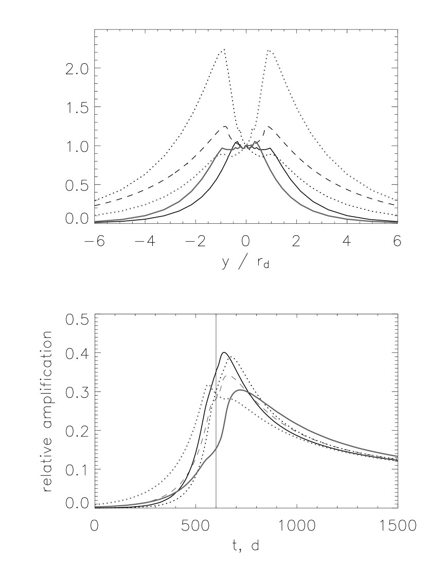
Figure 6: One-dimensional brightness distributions (upper panel) and amplification curves (lower panel) for a disc inclined by $60^{\circ}$ around a $a=0.6$ black hole. Dashed curve is the simplified disc model, black and grey curves correspond to caustic transition along the minor and major axes of the inclined disc (solid and dotted curves differ in propagation direction).

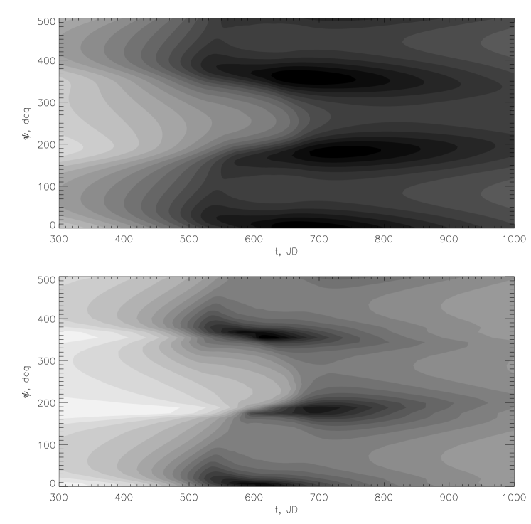
Figure 7: Amplification curves for an accretion disc around a black hole with $a=0.6$ inclined by $i=60^{\circ}$ (upper panel) and $i=85^{\circ}$ (lower panel) for variable positional angle $\psi$. Every horizontal slice corresponds to one curve. Scale is linear, maximal shade corresponds to maximal brightness.

Test runs reveal a small but considerable contribution from the photons belonging to the higher-order images produced by extreme light bending near the black hole (Beckwith & Done, 2005). Their contribution to the total flux may be as high as several percent, depending on the inclination and on the Kerr parameter. The figure of 10% given by Beckwith & Done (2005) is an over-estimate for an optically thick disc because at high inclinations and high Kerr parameters considerable part of the black hole is covered by the disc. Simulated black hole shadows with one higher-order image visible are shown in figure 8. Higher orders have significantly smaller fluxes due to gradually decreasing solid angle. Flux of $n$-th image loop decreases proportionally to its radial size $\Delta r$ (intensity is approximately conserved). During caustic crossing, the additional amplification factor is proportional to $\Delta r^{-1/2}$, where the observed projected width of the approximately annular image is $\propto\Delta r$. The resulting contribution of the $n$-th order image scales as $\propto\Delta r^{1/2}\propto\exp(-\pi n/b)$, where $b\simeq 2.7$ (in the so-called strong deflection limit, see Bozza (2010)). Higher-order images are thus exponentially damped.

An example of higher-order contribution is given in figure 9. For high inclinations, it is generally about a couple percent, but are less than one percent for $i\sim 0$ and $a>0$. For counter-rotating black holes, the size of the inner hole is the largest and the contribution of the secondary images reaches 2$..$3 percent for characteristic QSO black hole masses $\sim 10^{9}\mathrm{M_{\odot}}$. The effect is also important for larger black holes and at shorter wavelengths.

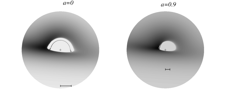
Figure 8: Black hole shadows for $i=80^{\circ}$ and two Kerr parameters, $a=0$ and $0.9$. Secondary image is clearly seen for Schwarzschild black hole and is visible as an inclined nearly straight line at the approaching (left) side in the other case. A bar below the black hole has the length equal to the innermost stable orbit radius (6 and $\sim$2.3 in $GM/c^{2}$ units, respectively).

Figure 9: Relative difference between the microlensing curves calculated in the single-image assumption and taking into account all the resolved secondary loops. We set $M=10^{10}\mathrm{M_{\odot}}$, $a=0$, $i=80^{\circ}$ and $\psi=0$ (solid line) and $90^{\circ}$ (dotted line). Effective transverse velocity is $v_{eff}=1000\mathrm{km\,s^{-1}}$, vertical line marks the instance of caustic crossing by the centre of the black hole.

4 Results

Fitting results with the simplified face-on disc and fully relativistic disc models are given in tables 2 and 3, respectively.

4.1 SBS J1520+530

Fitting with the plain face-on disc model allows to approximately recover the size of the inner hole. Number of degrees of freedom is $253-5=248$ here (“optimistic” number, see below). We fixed the mass of the black hole to $3\times 10^{9}\mathrm{M_{\odot}}$ and localized an absolute minimum near $a=-0.4$. Corresponding $X$ value is $1..2$. The minimum is consistent with physical $-1<a<1$ only for the black hole masses in the range $(1.6..3.5)\times 10^{9}\mathrm{M_{\odot}}$. The best-fit amplification curve is also shown in figures 10 and 11 by a dashed line. Here we limited the effective velocity by the value of $v_{eff,max}=2000\mathrm{km\,s^{-1}}$. If we relax this limitation, the fit may be improved (up to $\chi^{2}/DOF\sim 190$) by increasing the mass of the black hole and the transverse velocity.

A total number of 708 fully relativistic models was calculated covering the possible ranges of inclination $0<i<90\rm^{\circ}$, relative position angle $0<\psi<360\rm^{\circ}$ and Kerr parameter for co-rotating ($1>a>0$) and counter-rotating ($-1<a<0$) cases. For every model, we make an optimization run finding the best-fit $v_{eff}$ and $t_{0}$ and two amplification parameters $\mu_{0}$ and $\mu_{1}$. Thus the model one-dimensional brightness distribution fixes only the shape of the amplification curve that may be then stretched and shifted in time ($t_{0}$ and $v_{eff}$) and in amplification factors ($\mu_{0,1}$). For Kerr disc models, we first fix the mass of the black hole to $0.88\times 10^{9}\mathrm{M_{\odot}}$ and then, after finding the global minimum at $a=-0.9^{+0.4}_{-0.05}$, $i=80\pm 5\rm^{\circ}$ and $\psi=340\pm 4\rm^{\circ}$, fix $X$, $i$ and $\psi$ and vary the mass and rotation parameter.

In tables 2 and 3, we give the best fit parameters for the amplification curve of SBS J1520+530 fitted with the simplified disc model and with a Kerr disc with the best-fit parameters. Fully relativistic disc provides much better fit (see below this section). However, the observed details in the amplification curve are even sharper and more profound. This is a possible signature of a non-trivial structure of the inner parts of the disc resulting from either disc tilts and warps (see below section 5.4) or from additional energy input from black hole rotation (Agol & Krolik, 2000).

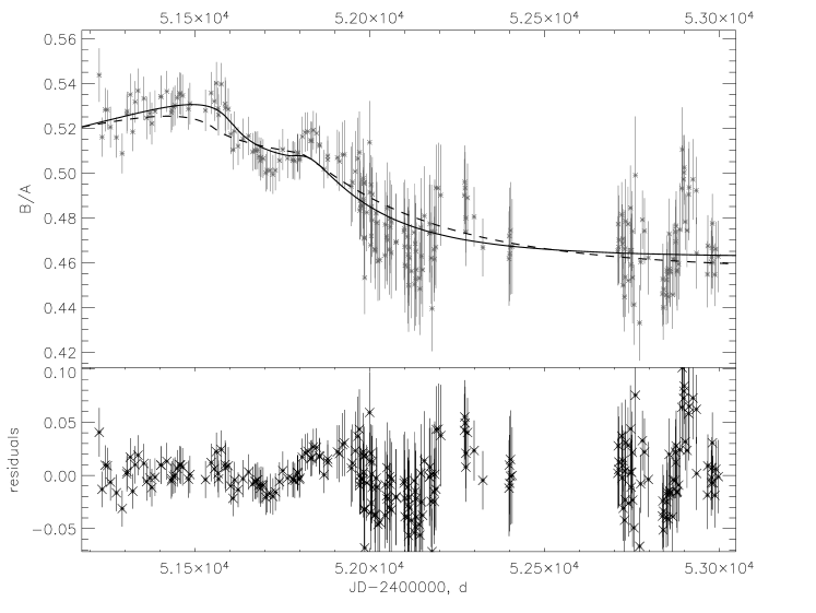
Figure 10: R-band B/A flux ratio for SBS J1520+530 fitted with a Schwarzschild face-on “plain disc” without relativistic effects (dashed curve) and a Kerr multi-blackbody disc of arbitrary inclination and spin (solid). The parameters of the best-fit Kerr disc model are: $a=-0.5$, $M=2\times 10^{9}\mathrm{M_{\odot}}$, $i=80^{\circ}$, $\psi=330^{\circ}$. Lower panel shows residuals with respect to the Kerr disc model.

The apparently low values of $\chi^{2}$ should be addressed separately. The procedure that we used to reproduce the amplification curve (see section 2) minimizes the loss of observational information but generates two sets of flux ratios (A image fluxes interpolated over the observational epochs for B and vice versa) that are not entirely independent. Therefore, the effective number of degrees of freedom (DOF) is not the number of flux ratio data points ($N_{F}=$253) minus the number of parameters ($N_{P}=5$ for simplified disc and $N_{P}=8$ for Kerr metric) but less. Therefore in the tables we give two estimates for the number of DOF: one optimistic $DOF_{1}=N_{F}-N_{P}$, and one pessimistic $DOF_{2}=N_{F}/2-N_{P}\simeq 120$. The real value is somewhere in between. For the simplified disc model, the number of parameters is less by 3 ($i$ and $\psi$ lacking, and $X$ instead of $a$ and $M$).

For both DOF estimates, the difference in $\chi^{2}$ is significant: F-test gives the probability of $7\times 10^{-10}$ (optimistic) and $4\times 10^{-5}$ (pessimistic DOF estimate) for the more sophisticated model to provide a better fit accidentally. The measured best-fit parameters, primarily the high inclination, are suspicious but not entirely unphysical. We propose that the real disc should be inclined with respect to the black hole plane and its inner parts should be thus strongly warped and distorted. In more detail we discuss this issue in section 5.4.

Table 2: Results of amplification curve fitting with the simplified accretion disc model. Effective velocity is normalised by the disc radial scale (R-band for SBS J1520+530, V-band for QSO J2237+0305) in $10^{15}\rm cm$ units.

	$r_{d}/r_{in}$	$v_{eff}/r_{d,15}$,$\mathrm{km\,s^{-1}}$	$t_{0}$, JD-2450000d	$\mu_{1}/\mu_{0}$	$\chi^{2}/DOF$
SBS J1520+530	1.5${}^{+0.6}_{-0.4}$	740${}^{+80}_{-60}$	1676.3${}_{-0.1}^{+4.7}$	1.05$\pm$0.17	209/246(120)
QSO J2237+0305 (A):
ISIS	$\begin{array}[]{l}2.0\pm 0.03\mbox{ (R)}\\ 1.6\pm 0.02\mbox{(V)}\\ \end{array}$	-2900$\pm 100$	1460$\pm 5$	$\begin{array}[]{l}2.4\pm 0.3\mbox{(R)}\\ 3.9\pm 0.4\mbox{(V)}\\ \end{array}$	560/99
PSF	$\begin{array}[]{l}2.6^{+0.13}_{-0.5}\mbox{ (R)}\\ 2.12^{+0.1}_{-0.4}\mbox{(V)}\\ \end{array}$	-2920$\pm 120$	1455.0$\pm 2$	$\begin{array}[]{l}4.5^{+0.06}_{-0.2}\mbox{(R)}\\ 6.0^{+0.09}_{-0.4}\mbox{(V)}\\ \end{array}$	122/96
QSO J2237+0305 (C)	$\gtrsim$4.4	6100${}_{-300}^{+400}$	1389.0${}^{+0.2}_{-0.1}$	0.66$\pm$0.02	183/77

Table 3: Results of amplification curve fitting with an inclined Kerr disc model.

$r_{d}/r_{in}$	$a$	$M$	$i$	$\psi$	$v_{eff}$	$t_{0}$	$\mu_{1}/\mu_{0}$	$\chi^{2}/DOF$
		$10^{9}\mathrm{M_{\odot}}$	deg	deg	$\mathrm{km\,s^{-1}}$	JD-2450000d
SBS J1520+530:
2.15$\pm$0.05	-0.6$..$0.2	1.7$..$3.4	80$\pm$10	335$\pm$5	1500$..$2400	1678$\pm$5	0.61$\pm$0.05	176/244(118)
QSO J2237+0305:
A image, ISIS
1.7$\pm$0.1 (R)	0.2${}^{+0.1}_{-0.2}$	7${}^{+2}_{-1}$	71${}^{+15}_{-5}$	96$\pm$5	$-(3\pm 1)\times 10^{4}$	$1509.9\pm 1.4$	0.91$\pm$0.06 (R)	333/96
1.4$\pm$0.1 (V)							0.92$\pm$0.03 (V)
A image, PSF
1.7${}^{+0.6}_{-0.02}$ (R)	-0.3$..$0.8	5${}^{+3}_{-2}$	70${}^{+10}_{-20}$	90${}_{-60}^{+30}$	$-(1.5..3.0)\times 10^{4}$	$1512^{+8}_{-5}$	0.96$\pm$0.07 (R)	98/93
1.4${}^{+0.5}_{-0.02}$ (V)							1.2$\pm$0.2 (V)
C image
2.1${}^{+0.7}_{-0.2}$	0.97$\pm 0.02$	$10_{-3}^{+10}$	85$\pm$5	53$\pm$10	$(2.0\pm 0.2)\times 10^{4}$	1309$\pm$4	2.09$\pm$0.05	88/75

An alternative to a single fold caustic amplifying a relativistic strongly-inclined disc is a more complex structure of several caustics or cusps. We find excellent agreement fitting the amplification curve with a simplified disc traversing two fold caustics sequentially in one direction at one velocity (figure 11). Best-fit parameters are, for fixed $a=0.2$ and $M=8.8\times 10^{8}\mathrm{M_{\odot}}$: $v_{eff}=(1.35\pm 0.22)\times 10^{4}\mathrm{km\,s^{-1}}$, $t_{01}=2451440\pm 12\rm d$ for the first fold and $t_{02}=2451810\pm 30\rm d$ for the second, the ratio of caustic strengths $l=0.84\pm 0.06$, $\chi^{2}=160/244(118)$. The strengths of the two caustics are about 0.7 and 0.6, the weaker one is delayed by $\Delta t=367\pm 8$ days. The worst problem for this interpretation of the observational data is the high required transverse velocity. Spatial size of the disc is $\propto M^{2/3}$, and the mass should be sufficiently decreased to match the required transverse velocity to the observed peculiar velocity distribution for galaxies. Setting $M=3\times 10^{8}\mathrm{M_{\odot}}$ allows to obtain a reasonable fit ($\chi^{2}\simeq 162$) for a relatively small transverse velocity $v_{eff}\sim 2\times 10^{3}\mathrm{km\,s^{-1}}$.

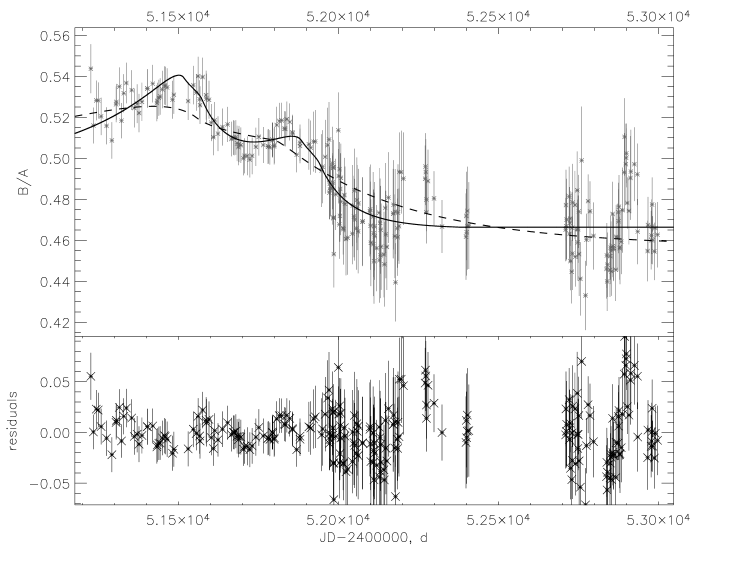
Figure 11: R-band B/A flux ratio for SBS J1520+530 fitted with a double-fold model (the best-fit curve parameters are given in the text, section 4.1). Simplified disc single-fold model curve is shown for comparison by a dashed curve.

4.2 QSO J2237+0305

Simplified disc fits appear even worse for the case of QSO J2237+0305. Qualitatively, the situation is understandable: plain disc symmetric brightness distribution is unable to reproduce the two-peak structure of image A event as well as the narrow peak feature of the image C event. Both are relatively well reproduced if the inclination is high ($i\gtrsim 70^{\circ}$).

Running more than 2000 models, we find a reasonable fit for the A image amplification curve (figure 12). For fitting, we use GLITP data reduced by the two standard techniques separately. PSF-fitting data have larger (but probably more reliable) statistical errors hence the minimal $\chi^{2}$ is considerably smaller. Higher rotation parameters (up to $\sim 0.9$) and higher masses (up to $\sim 10^{10}\mathrm{M_{\odot}}$) produce apparently worse fits but are still allowed if one increases the observational uncertainties by a factor of several. Inclination $i$ and positional angle $\psi$ are well constrained, because the notable two-peak structure requires certain disc orientation (see figure 7). At the moment we are satisfied with the qualitative agreement because the data definitely have some additional error sources possibly connected to the bad visibility of the object near the amplification curve maximum. Amplification curve shape is similar for both filters, even the two maxima seen in the R-band curve are also visible in the V-band.

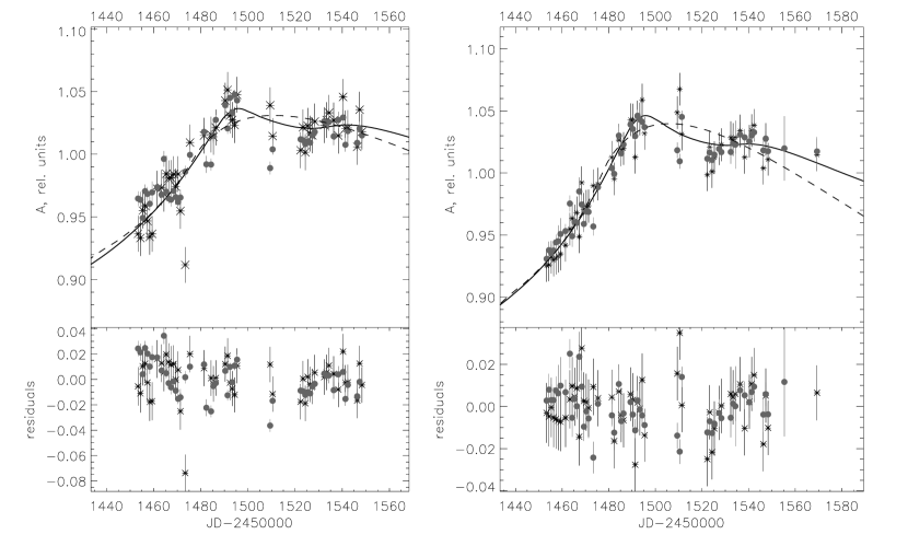
Figure 12: Amplification curve for the A image of QSO J2237+0305 fitted with a Kerr disc fold traversal model with $a=0.2$, $M=7\times 10^{9}\mathrm{M_{\odot}}$, $i=70^{\circ}$, $\psi=96^{\circ}$. R band is to the left, V band to the right. Simplified disc best fit is shown for comparison by a dashed curve. Asterisks and circles correspond to ISIS and PSF-fitting fluxes, respectively.

It is impossible to explain the observed amplification curve of the C image without a relatively large $a\gtrsim 0.95$. The rapid rise of the curve in figure 13 can not be reproduced unless the accretion disc has a bright spot naturally explained by high rotation parameter, high mass models. The predicted mass is very high, $M\gtrsim 7\times 10^{9}\mathrm{M_{\odot}}$. If the C-image amplification is a bona fide caustic crossing event, then virial mass measurements underestimate the masses of quasars by a factor of several.

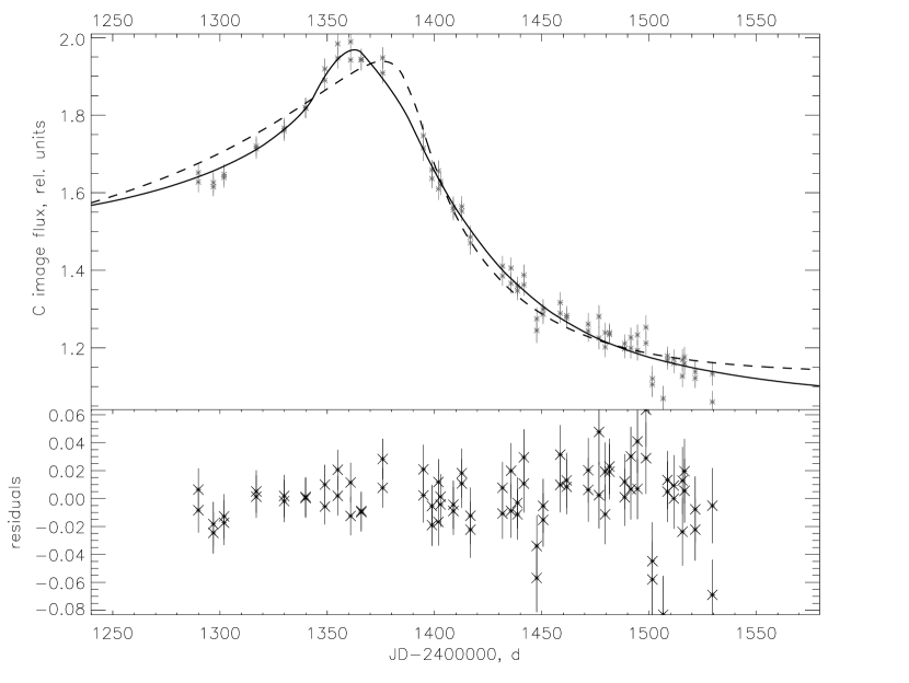
Figure 13: Best fit for the QSO J2237+0305 image C high amplification event, V band. Simplified disc fit is shown by a dashed line, solid line is the best-fit Kerr metric disc fit ($a=0.97$, $M=10^{10}\mathrm{M_{\odot}}$, $i=85^{\circ}$ and $\psi=53^{\circ}$).

5 Discussion

5.1 What do caustic crossings really probe for?

The fine structure of high-amplification events in the light curves of microlensed quasars is an effect naturally expected in the framework of thin accretion disc model. Replacing accretion disc brightness distribution by some symmetrical structure with brightness uniformly decreasing with distance would produce a light curve with a single nearly symmetrical peak with the duration time scale $r_{d}/v_{eff}$ defined by the size of the emitting region (see for example the analytical solutions given in Schneider & Weiss (1987), Appendix B). Its shape near the maximum is roughly parabolic. In this case, the amplification curve maximum is always convex unless the brightness distribution has a non-monotonic or asymmetric shape. Interpreting individual humps in the amplification curves as individual caustic crossing events leads to unphysically large transverse velocities several times larger than the upper limits estimated in section 3.1.

As it was shown in section 3.2, the only parameter affecting the amplification curve shape in the simplified disc case is $X=r_{d}/r_{in}$. Disc size scale itself is degenerate with the effective transverse velocity. Amplification curves are primarily sensitive to the combinations $r_{in}/v_{eff}\sqrt{J}$ and $r_{d}/v_{eff}\sqrt{J}$ (see section 3.2) having the physical meaning of traversal times for the central hole in the disc and the disc radial scale itself, respectively. This also holds for the general relativistic case as long as the disc is nearly face-on.

Relativistic effects break these degeneracies at inclinations $i\gtrsim 60^{\circ}$. Amplification curve properties become sensitive to the two angles $i$ and $\psi$, but the dependence on $a$ is weaker and similar light curves emerge for similar values of $X$ if inclination and positional angle are the same.

Interpretation of the three events relies on their consideration as caustic-crossing events. For QSO J2237+0305, this is justified by the works of Gil-Merino et al. (2006); Koptelova et al. (2007) who performed detailed simulations to check whether artificial amplification maps produce caustic crossings similar (in some sense) to the observed peaks in the light curves of individual images.

For the case of SBS J1520+530, optical depths to microlensing are relatively small. Central convergence of $\kappa_{c}=0.5$ sets an absolute upper limit for it. The optical depth to microlensing is smaller than $\kappa_{c}$ unless the stars in the optical path are strongly clumped, that is unlikely for an elliptical galaxy (probability of accidentally hitting a globular cluster is $\sim 10^{-5}$). If dark matter makes significant contribution to the gravitational field of the lensing galaxy, optical depths should be decreased proportionally toward the probable value of $\sim 0.1$ for the stronger lensed B image. Image A is about three times farther from the centre of the lens that makes it much worse candidate for microlensing. The caustic net structure in this case is determined by small shears distorting single-lens amplification patterns (Kofman et al., 1997). Therefore, there is a strong probability for passing a close caustic pair. However, in this case the caustics are traversed in opposite directions that should produce a pattern completely different from the observed amplification curve.

In this work, we used Kerr-metric geodesics and relativistic Doppler effects, but the disc model was not fully relativistic. We used the temperature law of Shakura & Sunyaev (1973) instead of the more accurate relativistic thin disc law provided by Novikov & Thorne (1973); Page & Thorne (1974). Difference in the two laws is in the correction factor that decays more smoothly inwards and is generally smaller for the fully relativistic thin disc case. We tested the difference between the amplification curves calculated using these two temperature laws and found that for relevant black hole parameters ($M\lesssim 10^{10}\mathrm{M_{\odot}}$ and $a>-0.9$), the difference is smaller than one percent of the peak amplification. It is more important to consider the effects of non-trivial inner boundary condition, shock formation and rapid disc tilt change in the inner parts of the disc and then pass to finer effects like the general relativity corrections to the temperature law.

5.2 Caustic strengths

For SBS J1520+530, amplification curve amplitude is moderate and may be characterised by a caustic strength of $k=\mu_{1}/\mu_{0}\sim 0.6$. Using the estimates made by Witt et al. (1993), one may expect a mean caustic strength of:

$$\langle k\rangle\sim 0.56\left(\langle m\rangle/\tau\right)^{1/4},$$ (20)

where $\tau\simeq 0.1..0.5$ is the optical depth to microlensing, and $\langle m\rangle\sim 0.1..0.5$ is the mean microlens mass in Solar units. Note that the dependence is very weak both on the optical depth and on the mean mass thus making the caustic strength a good consistency check for the model. In the case of SBS J1520+530, observational data argue for $\langle m\rangle/\tau\sim 1$, consistent with a moderately sub-solar mean stellar mass. Low end of the mass function of red and brown dwarfs is poorly known and probably variable (Bastian et al., 2010). There are indications for a low mean stellar/substellar mass ($\langle m\rangle\sim 0.1$) in the old stellar population of elliptical galaxies (van Dokkum & Conroy, 2010), therefore the optical depth to microlensing is most likely relatively small, $\tau\sim 0.1$. If the amplification curve for SBS J1520+530 is interpreted as a superposition of two caustic crossings, the two folds have similar strengths of 0.7 and 0.6, consistent as well with a stellar population rich in low-mass objects.

For QSO J2237+0305 events, the amplitudes are higher. Qualitatively, it was expected, because the lens is a spiral galaxy and the number of massive stars among the microlenses should be higher, with the mean mass of $\sim 1\mathrm{M_{\odot}}$. Mean caustic strength $\langle k\rangle\simeq 2$ (as for the image C event) only if $\langle m\rangle/\tau\sim 100\mathrm{M_{\odot}}$ and hence $\langle m\rangle\sim 40\mathrm{M_{\odot}}$ (numerical simulations suggest that the optical depth to microlensing is $\tau\sim 0.4$ for Einstein’s cross (Bate et al., 2011)) that is considerably higher than what one may expect even from a young stellar population. In most simulations with $\tau\sim 0.5$ (see for example Schechter & Wambsganss (2002); Schechter et al. (2004)), predicted amplification factor distributions are broad and allow caustics with strengths exceeding the mean value of $k$ by a factor of $\sim 2$. The reason why our estimates do not contradict the theory is selection effect: we consider two brightest and most evident high amplification events while the total number of fainter events present in the light curves of the four images in the about three-year interval of OGLE-II monitoring program is about 10 (if the mean distance between fold traversals is about a year).

5.3 Black hole masses and disc sizes

The relative size of the inner disc hole and the observed strength of relativistic effects favour black hole masses significantly higher than virial estimates. For SBS J1520+530 and QSO J2237+0305, the virial masses estimated using the width of the CIV$\lambda$1549 resonance line are equal to $8.8\times 10^{8}$ (Peng et al., 2006) and $9\times 10^{8}\mathrm{M_{\odot}}$ (Yee & De Robertis, 1991), correspondingly, with the proposed uncertainty of about a factor of 2. Single caustic crossing event fitting argues for considerably higher masses, $(2..3)\times 10^{9}\mathrm{M_{\odot}}$ and $(7..9)\times 10^{9}\mathrm{M_{\odot}}$.

Altering black hole masses by a factor of $\sim 3$ was proposed by Morgan et al. (2010) to explain the inconsistency between the accretion disc sizes estimated using microlensing statistics and the accretion disc size predictions following from the standard disc theory. Note that in our study the degeneracies are different from those in Morgan et al. (2010). While the Monte Carlo light curve analysis is sensitive to the disc size itself ($r_{d}\propto\left(l/\eta\right)^{1/3}M^{2/3}$), the shapes of caustic-traversal events primarily reflect the ratio of the disc radial size scale to its inner boundary size ($X\propto\left(l/\eta\right)^{1/3}M^{-1/3}$). To reproduce our results without altering black hole masses we should decrease the Eddington ratio by a factor of several rather than accretion efficiency as it was proposed by Morgan et al. (2010).

To distinguish between higher black hole masses and lower $l/\eta$ ratios, one may use either photometrical data or different-technique accretion disc size estimates. Central black hole mass may be estimated using amplification-corrected magnitudes. Observed flux from a thin disc is calculated by integrating the observed intensity (indices “obs” and “em” refer here to the radiation intensity in the observer frame and in the frame comoving with the QSO):

$$\begin{array}[]{l}F_{\nu}=\int I_{\nu,obs}d\Omega=\\ \qquad{}=\frac{2\pi}{D^{2}\times(1+z)^{3}}\cos i\times\int I_{\nu,em}\left(\nu/(1+z)\right)RdR,\end{array}$$

where $D=D(z)$ is angular size distance. This distance scale is known for its non-monotonic dependence on redshift. Maximal distance of $1.7\mathrm{Gpc}$ is reached at the intermediate redshift of $z\simeq 1.6$ for standard $\Lambda$CDM. Most of the well-studied lensed quasars have redshifts close to this value.

For $I_{\nu}$, we substitute the Planck law with the temperature law determined by the standard accretion disc theory as:

$$T=\left(\frac{3}{2}\frac{G^{2}M^{2}}{\sigma\kappa c}\frac{l}{\eta}\right)^{1/4}R^{-3/4}$$

Here we neglect the correction term that has only small influence on the integral flux since the area of the disc affected by the term is about $(r_{in}/2.44r_{d})^{2}\lesssim 0.1$ times smaller. For the integration limits set to 0 and $+\infty$, the integral is reduced to the following (Abramowitz, M. & Stegun, I. A., 1972):

$$\int_{0}^{+\infty}\frac{x^{5/3}dx}{e^{x}-1}=\Gamma(8/3)\zeta(8/3)$$

Observed flux is finally expressed as:

$$\begin{array}[]{l}F_{\nu}=\frac{4\pi h\nu_{em}^{3}}{c^{2}}\frac{\cos i}{D^{2}\times(1+z)^{3}}\int\frac{RdR}{\exp\left(\frac{h\nu}{kT(R)}\right)-1}=\\ \qquad{}=8\pi\left(\frac{2}{3}\right)^{1/3}\Gamma(8/3)\zeta(8/3)\frac{k^{8/3}\nu_{obs}^{1/3}}{c^{8/3}h^{5/3}\kappa^{2/3}\sigma^{2/3}}\times\\ \qquad{}\times(GM)^{4/3}\left(\frac{l}{\eta}\right)^{2/3}\cos i\times\frac{1}{D^{2}\times(1+z)^{8/3}}\simeq\\ \qquad\simeq 6.9\cos i\left(\frac{l}{\eta}\right)^{2/3}\left(\frac{\lambda_{obs}}{1\mu}\right)^{-1/3}\left(\frac{M}{10^{9}\mathrm{M_{\odot}}}\right)^{4/3}\times\\ \qquad{}\times\left(\frac{D}{1\mathrm{Gpc}}\right)^{-2}(1+z)^{-8/3}\mathrm{mJy}\end{array}$$

This flux may be used to independently estimate the black hole mass. In particular, for the HST F814W filter (we used the calibration given in Holtzman et al. (1995); this allows to use the magnitudes given by Morgan et al. (2010) in table 1) the mass may be estimated photometrically as follows:

$$\begin{array}[]{l}M\simeq 2.7\times 10^{7}\left(\frac{D}{1\mathrm{Gpc}}\right)^{3/2}(1+z)^{2}\times\\ \qquad{}\times\sqrt{\frac{\eta}{l}}\cos^{-3/4}i\times 10^{-0.3(I-19)}\mathrm{M_{\odot}}\\ \end{array}$$ (21)

Following the original work where a similar formula was used to estimate the photometrical radius, we denote the magnitude by $I$ and use the amplification-corrected values of $I(QSO~{}J2237+0305)=17.9\pm 0.44\,\!^{\rm m}$ and $I(SBS~{}J1520+530)=18.92\pm 0.13\,\!^{\rm m}$. Photometrical masses are closer to the virial mass estimates. These estimates are degenerate with the $l/\eta$ ratio in a way different from the results of our light-curve analysis that allows to reach consistency if the Eddington ratio is low, $l/\eta\sim 0.1$. In figure 14, we show the estimates for $l/\eta$ and black hole mass made with different methods. Monte-Carlo amplification curve fitting is sensitive to $r_{d}\propto M^{2/3}\times(l/\eta)^{1/3}$, while the observed amplification-corrected flux scales as $F_{\nu}\propto M^{4/3}\times(l/\eta)^{2/3}$ that results in parallel bands in the graph. For QSO J2237+0305, the microlensing and photometrical radii are consistent within the uncertainties. Our data may be made consistent with photometry and virial masses for narrow ranges of parameter values. In particular, for QSO J2237+0305, there is a zone where all the three bands intersect, $M\simeq(1.6..1.8)\times 10^{9}\mathrm{M_{\odot}}$ and $l/\eta\simeq 0.5..0.6$. In the case of SBS J1520+530, photometry, virial and light-curve fitting intersect for $M\simeq(0.8..1.1)\times 10^{9}\mathrm{M_{\odot}}$ and $l/\eta\simeq 0.7..1.3$. However, in this case the microlensing radius found by Morgan et al. (2010) is considerably higher.

Consistency between different methods of radius and mass estimates allows to suggest that the microlensing radii found by Morgan et al. (2010) are a subject to some bias that increases in some cases the effective radius by a factor of several. This may be contamination from a source of much larger angular size (such as unresolved starlight or the broad-line region) or some optically-thin scatterer. These effects were considered in the original work and seem to qualitatively explain the observed discrepancy.

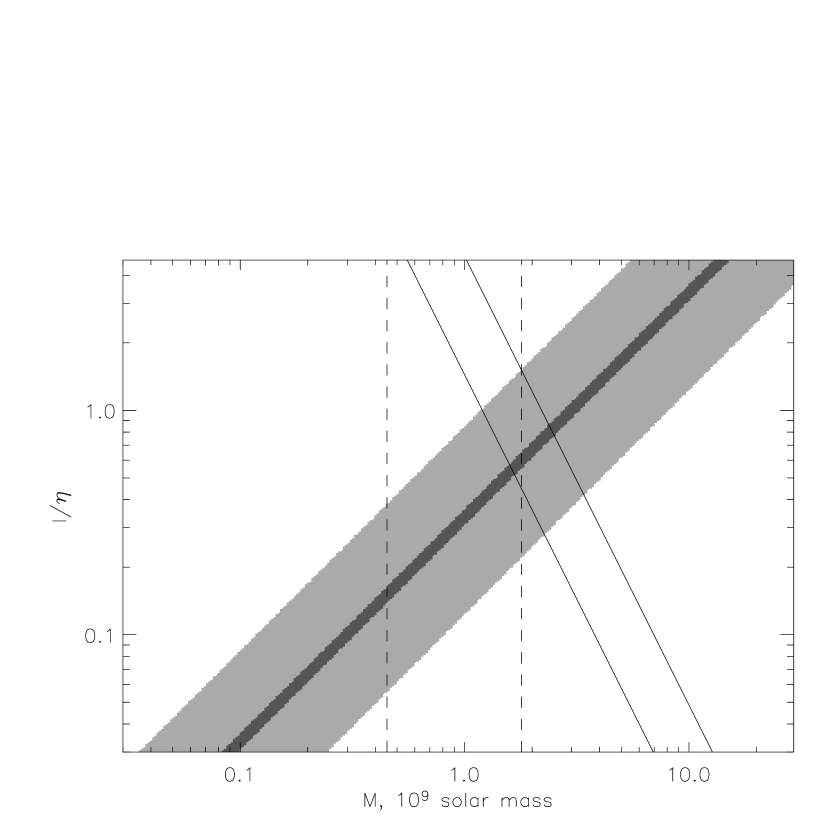
Figure 14: Mass and $l/\eta$ for QSO J2237+0305. Shaded region is the band restricted by the light curve fitting made in the present work (the darkest region corresponds to the intersection of the both mass estimates). Vertical dashed lines show the range set by the virial mass estimate with the relative uncertainty of $0.3\rm dex$. Solid lines show the constraints set by equation (21). Disc inclination is set to $60^{\circ}$.

Since in general there are inconsistencies between the accretion disc radii obtained by different methods, we refrain from any final conclusions upon the masses of the central black holes in QSO discs. Still it seems plausible that the apparently large disc sizes may be connected to larger black hole masses, smaller Eddington ratios and high inclinations (the issue of these will be considered in detail in the next subsection). We also do not exclude that some non-standard accretion regimes may influence the observational properties of quasar accretion discs. In particular, low accretion rates may lead to an optically-thin advection dominated region in the inner parts of the disc. The innermost stable orbit radius will be over-estimated in this case resulting in black hole masses and accretion disc sizes biased toward higher values. We will consider the effects of non-standard accretion regimes on microlensing variability in subsequent papers.

Larger black hole masses mean also larger disc sizes. For black hole masses $M\sim 10^{10}\mathrm{M_{\odot}}$, disc size in the considered wavelength range becomes $\sim 10^{16}\rm cm$ that is comparable to the Einstein radius $r_{Ein}$ in the case of SBS J1520+530. Straight caustic approximation is violated in this case because $\theta_{Ein}$ also sets the mean curvature radius of fold caustics as well as the mean distance between individual folds for intermediate $\tau$ (Gaudi & Petters, 2002). For the case of QSO J2237+0305, Einstein-Chwolson radius is larger because of the smaller distance $D_{L}$. Most of the results of this work refer to the inner parts of the disc that makes the effects of caustic curvature even smaller. For future more accurate studies, we propose using the more precise parabolic model (Fluke & Webster, 1999).

5.4 Inclinations of QSO discs

High inclinations ($i\gtrsim 70^{\circ}$) are required if we interpret the three considered high amplification events as caustic crossings. All the three events show fine structure near their maxima. It is possible to explain this by highly inclined, relativistic discs around black holes with masses considerably higher than the virial estimates. One amplification curve (QSO J2237+0305, image C) allows to restrict both the Kerr parameter and the mass to a high accuracy. Still it should be noted that these estimates are sensitive to the inner structure of the disc and therefore model-dependent. High inclinations are needed because the observational data require asymmetric brightness distributions.

Still, there are strong reasons why QSO discs should not be inclined by $\gtrsim 70^{\circ}$:

• Outer disc rim has a non-negligible thickness and is able to obscure the central UV-radiating parts if inclination is $i\gtrsim\pi/2-h/R$, where $h/R\sim 0.02$ is the relative disc thickness (Shakura & Sunyaev, 1973); this is important if the disc has very high inclination $i\gtrsim 85^{\circ}$.

• A stricter limit is set by dust tori detected spectrally for most quasars. Hot dust emission is observed from QSO J2237+0305 (Agol et al., 2000) consistent with a large-scale ($R\gtrsim 0.03\mathrm{pc}$) structure of dust intercepting considerable part of the quasar luminosity and re-radiating the absorbed luminosity in the infrared range.

• A disc observed edge-on should appear under-luminous. For a thin disc, the observed luminosity is $\cos i$ times lower than for the face-on case, for a concave disc the decrease is stronger. Thus the real luminosity should be a factor of $\cos^{-1}i\sim 10$ higher. In the case of QSO J2237+0305, a strong observational evidence for small inclination ($i>60^{\circ}$ is ruled out at a 95% confidence level) is given in Poindexter & Kochanek (2010).

The strength of the last argument is diminished by the high inferred masses of the central black holes. An order of magnitude higher black hole mass leads to an order of magnitude higher Eddington luminosity. This makes the observed flux consistent with the microlensing disc size estimates. Besides, Poindexter & Kochanek (2010) did not consider relativistic effects that have the potential to distort the dependence of the observed flux on inclination significantly. For the moderate black hole mass of $10^{9}\mathrm{M_{\odot}}$ and $a=0.6$, luminosity dependence on inclination deviates by more than 20% at $i>40\rm^{\circ}$ and by more than 50% at $i>70\rm^{\circ}$ (see figure 15).

Figure 15: Flux dependence on inclination for an accretion disc around an $M=10^{9}\mathrm{M_{\odot}}$, $a=0.6$ black hole. Dotted line shows the $\cos i$ law for comparison.

An interesting clue is that SBS J1520+530 is a BAL (broad absorption line) quasar (Chavushyan et al., 1997). Though BAL QSO are generally considered as seen nearly edge-on (Elvis, 2000), some of these objects have strongly variable bright radio emission suggesting a collimated relativistic outflow observed at low inclination (Zhou et al., 2006). It is still an open question how one can collimate a jet in a direction different from the normal to the disc plane.

A possible solution is that the angular momenta of the accreting black holes in SBS J1520+530 and QSO J2237+0305 are misaligned with the angular momentum of the infalling matter. Since there are no reasons for a supermassive black hole to be aligned with the accreting matter at large distances, this is probably the case. The inner parts of the flow should be tilted and warped. Most investigations predict alignment of the inner parts of the flow known as Bardeen-Petterson effect, see Bardeen & Petterson (1975), normally inside the $R\sim 10\,r_{in}$ region where the observed UV radiation is emitted. Similar misalignment may be proposed a possible reason for the apparent inconsistency between the inclinations inferred from radio and optical properties of radio-loud BAL quasars.

Figure 16: Simulated amplification curves of an inclined (solid line) and tilted (dotted) discs. For both curves, $a=0.9$, $M=10^{9}\mathrm{M_{\odot}}$, maximal inclination is 80^∘, $\psi\simeq 0$, $v_{eff}=-10000\mathrm{km\,s^{-1}}$. See section 5.4 for details.

In figure 16 we show the predicted amplification curve for a thin accretion disc with zero inclination at infinite distance but tilted toward the plane of the black hole inclined by $\theta_{bh}$ to the picture plane (and to the plane of the disc at large distances). For inclination, we use the law $\theta(r)=\theta_{bh}\cdot\exp\left(-r/r_{in}\right)$. Rotation law for an inclined disc was taken from Shakura (1987), while the temperature law was assumed standard. Every annulus was considered flat that is of course an over-simplification but still serves the main goal to show that fold caustic traversal curves are primarily sensitive to the innermost parts of the accretion disc.

5.5 Influence of disc tilts upon the unification scheme

In case of random orientation of the black hole spin and the orbital angular momentum of the matter entering the disc, an average disc will have a tilt of $\theta\sim 90^{\circ}$ at large distances. Half of the discs should be counter-rotating. In case of random misalignment, half of the disc planes should have inclinations larger than 60^∘ with respect to the black hole rotation frame. A tilted disc around a Kerr black hole is usually proposed to gradually change its inclination with decreasing radius approaching alignment at the innermost stable orbit Linear analysis made by Zhuravlev & Ivanov (2011) for a thin disc around a nearly-Schwarzschild black hole confirms this conclusion only for the case of considerably large viscosity (see the original work for details). The authors also show stability of counter-rotating discs around slowly rotating black holes. On the other hand, numerical simulations made by Fragile & Anninos (2005); Dexter & Fragile (2011) suggest that the disc evolution toward alignment should take place in its innermost parts, at several Schwarzschild radii.

Tilted discs may become a serious obstacle for formation and observability of relativistic jets. Once formed, relativistic outflows will be stopped by the higher-pressure material of the disc or the dust torus. If jet formation and propagation into the rarefied galactic medium becomes impossible in case of strongly inclined discs, one may try to explain the observed radio brightness dichotomy of QSO by different regimes of alignment, as it was proposed by Lawrence & Elvis (2010) for Seyferts and radiogalaxies. Presence of a thick torus with $\theta_{t}\sim 30^{\circ}$ leads to about 75% probability that the jet will be stopped either by the torus or by the tilted disc itself. The real fraction of radio-weak sources is higher, about 90% (see for example Hewett et al. (2001)).

Importance of disc tilts for jet formation may also have connection to the formation of the “localised” X-ray radiation found in some QSO. In particular, in the two recent works by Zimmer et al. (2011) and Chen et al. (2011), the properties of the X-ray emitting region in QSO J2237+0305 are recovered using microlensing curves. In Chen et al. (2011), it is concluded that this region is smaller and more variable than any existing extended jet or corona model can explain. Among other possibilities, the “failed jet” model by Ghisellini et al. (2004) is put forward. If the jet possesses enough energy to escape the gravitational well but is stopped by the disc matter, the source of the X-ray emission may be connected to the hot spot in the disc where its energy is dissipated. Relativistic termination shock remains invisible but the bow shock where the ram pressure is balanced by the pressure of the disc should make important contribution to the observed X-ray emission. And the spatial size of the X-ray bright spot may be small if the jet is sufficiently collimated. Stopped jet model may be checked by considering correlations between different properties of X-ray and radio emission from quasars.

6 Conclusions

We show that general relativity effects have considerable influence on the amplification curves of microlensed quasars. This effect is more profound if the disc is strongly inclined. Having better data on hand (smaller observational errors, larger homogeneity and better temporal coverage) may allow to resolve the structure of high-amplification events with a better precision and to use them for accurately measuring disc tilts and black hole rotation parameters of lensed quasars.

Some implications may be made even now. In particular, the discs in both objects, SBS J1520+530 and QSO J2237+0305, are seen at high inclinations. Apparent contradiction with the high observed fluxes and lack of strong absorption signatures in the spectra may be resolved if one considers a disc having low inclination ($i\lesssim 60^{\circ}$) at tens of $GM/c^{2}$ but is seen nearly edge-on in its inner parts. Similar picture is expected if the initial angular momentum of the accreted matter is strongly misaligned with that of the black hole.

High probability to effectively measure a high inclination may be qualitatively understood as a very strong tilt and warp near the last stable orbit. In this case, there should be, at a high probability, some radius at which the disc lies perpendicular to the picture frame. Contribution of this annulus should be enhanced by Doppler boost. In other words, if a disc has a range of inclinations due to tilts and warps, higher inclinations will make larger contribution to microlensing amplification curves.

In the analysed data we do not find any challenges for the standard accretion disc model. But they bring our attention toward the role of disc tilts that was never considered in the framework of QSO microlensing. Besides, some of accretion disc properties are better understood if we alter the accretion disc parameters such as Eddington ratio and accretion efficiency. The apparently high black hole masses and disc sizes required by microlensing effects may be connected to the low accretion efficiency and contamination by larger angular scales.

Note added in proof:

We became aware of the papers by Bogdanov & Cherepashchuk (2002, 2004) where amplification curves considered in this work were analysed. Authors restore one-dimensional brightness distributions and propose to connect their shapes to relativistic effects.

References

- Abramowitz, M. & Stegun, I. A. (1972) Abramowitz, M. & Stegun, I. A. ed. 1972, Handbook of Mathematical Functions. New York: Dover
- Agol et al. (2000) Agol E., Jones B., Blaes O., 2000, ApJ, 545, 657
- Agol & Krolik (1999) Agol E., Krolik J., 1999, ApJ, 524, 49
- Agol & Krolik (2000) Agol E., Krolik J. H., 2000, ApJ, 528, 161
- Alcalde et al. (2002) Alcalde D., Mediavilla E., Moreau O., Muñoz J. A., Libbrecht C., Goicoechea L. J., Surdej J., Puga E., De Rop Y., Barrena R., Gil-Merino R., McLeod B. A., Motta V., Oscoz A., Serra-Ricart M., 2002, ApJ, 572, 729
- Auger et al. (2008) Auger M. W., Fassnacht C. D., Wong K. C., Thompson D., Matthews K., Soifer B. T., 2008, ApJ, 673, 778
- Bardeen & Petterson (1975) Bardeen J. M., Petterson J. A., 1975, ApJL, 195, L65+
- Bardeen et al. (1972) Bardeen J. M., Press W. H., Teukolsky S. A., 1972, ApJ, 178, 347
- Barkhouse & Hall (2001) Barkhouse W. A., Hall P. B., 2001, AJ, 121, 2843
- Bastian et al. (2010) Bastian N., Covey K. R., Meyer M. R., 2010, ARA&A, 48, 339
- Bate et al. (2008) Bate N. F., Floyd D. J. E., Webster R. L., Wyithe J. S. B., 2008, MNRAS, 391, 1955
- Bate et al. (2011) Bate N. F., Floyd D. J. E., Webster R. L., Wyithe J. S. B., 2011, ApJ, 731, 71
- Beckwith & Done (2005) Beckwith K., Done C., 2005, MNRAS, 359, 1217
- Blackburne et al. (2011) Blackburne J. A., Pooley D., Rappaport S., Schechter P. L., 2011, ApJ, 729, 34
- Bogdanov & Cherepashchuk (2002) Bogdanov M. B., Cherepashchuk A. M., 2002, Astronomy Reports, 46, 626
- Bogdanov & Cherepashchuk (2004) Bogdanov M. B., Cherepashchuk A. M., 2004, Astronomy Reports, 48, 261
- Bozza (2010) Bozza V., 2010, General Relativity and Gravitation, 42, 2269
- Burud et al. (2002) Burud I., Hjorth J., Courbin F., Cohen J. G., Magain P., Jaunsen A. O., Kaas A. A., Faure C., Letawe G., 2002, A&A, 391, 481
- Chang & Refsdal (1984) Chang K., Refsdal S., 1984, A&A, 132, 168
- Chavushyan et al. (1997) Chavushyan V. H., Vlasyuk V. V., Stepanian J. A., Erastova L. K., 1997, A&A, 318, L67
- Chen et al. (2011) Chen B., Dai X., Kochanek C. S., Chartas G., Blackburne J. A., Kozłowski S., 2011, ApJL, 740, L34
- Dexter & Agol (2009) Dexter J., Agol E., 2009, ApJ, 696, 1616
- Dexter & Fragile (2011) Dexter J., Fragile P. C., 2011, ApJ, 730, 36
- Eigenbrod et al. (2008) Eigenbrod A., Courbin F., Meylan G., Agol E., Anguita T., Schmidt R. W., Wambsganss J., 2008, A&A, 490, 933
- Eigenbrod et al. (2008) Eigenbrod A., Courbin F., Sluse D., Meylan G., Agol E., 2008, A&A, 480, 647
- Elvis (2000) Elvis M., 2000, ApJ, 545, 63
- Floyd et al. (2009) Floyd D. J. E., Bate N. F., Webster R. L., 2009, MNRAS, 398, 233
- Fluke & Webster (1999) Fluke C. J., Webster R. L., 1999, MNRAS, 302, 68
- Fragile & Anninos (2005) Fragile P. C., Anninos P., 2005, ApJ, 623, 347
- Gaudi & Petters (2002) Gaudi B. S., Petters A. O., 2002, ApJ, 574, 970
- Gaynullina et al. (2005) Gaynullina E. R., Schmidt R. W., Akhunov T., Burkhonov O., Gottlöber S., Mirtadjieva K., Nuritdinov S. N., Tadjibaev I., Wambsganss J., Wisotzki L., 2005, A&A, 440, 53
- Ghisellini et al. (2004) Ghisellini G., Haardt F., Matt G., 2004, A&A, 413, 535
- Gil-Merino et al. (2006) Gil-Merino R., González-Cadelo J., Goicoechea L. J., Shalyapin V. N., Lewis G. F., 2006, MNRAS, 371, 1478
- Hainline et al. (2012) Hainline L. J., Morgan C. W., Beach J. N., Kochanek C. S., Harris H. C., Tilleman T., Fadely R., Falco E. E., Le T. X., 2012, ApJ, 744, 104
- Hewett et al. (2001) Hewett P. C., Foltz C. B., Chaffee F. H., 2001, AJ, 122, 518
- Hogg (1999) Hogg D. W., 1999, ArXiv Astrophysics e-prints, 9905116
- Holtzman et al. (1995) Holtzman J. A., Burrows C. J., Casertano S., Hester J. J., Trauger J. T., Watson A. M., Worthey G., 1995, PASP, 107, 1065
- Huchra et al. (1985) Huchra J., Gorenstein M., Kent S., Shapiro I., Smith G., Horine E., Perley R., 1985, AJ, 90, 691
- Irwin et al. (1989) Irwin M. J., Webster R. L., Hewett P. C., Corrigan R. T., Jedrzejewski R. I., 1989, AJ, 98, 1989
- Jaroszynski et al. (1992) Jaroszynski M., Wambsganss J., Paczynski B., 1992, ApJL, 396, L65
- Jimenez-Vicente et al. (2012) Jimenez-Vicente J., Mediavilla E., Muñoz J. A., Kochanek C. S., 2012, ArXiv e-print 1201.3187
- Kayser & Witt (1989) Kayser R., Witt H. J., 1989, A&A, 221, 1
- Khamitov et al. (2006) Khamitov I. M., Bikmaev I. F., Aslan Z., Sakhibullin N. A., Vlasyuk V. V., Zheleznyak A. P., Zakharov A. F., 2006, Astronomy Letters, 32, 514
- Kochanek (2004) Kochanek C. S., 2004, ApJ, 605, 58
- Kofman et al. (1997) Kofman L., Kaiser N., Lee M. H., Babul A., 1997, ApJ, 489, 508
- Koptelova et al. (2007) Koptelova E., Shimanovskaya E., Artamonov B., Yagola A., 2007, MNRAS, 381, 1655
- Koptelova et al. (2006) Koptelova E. A., Oknyanskij V. L., Shimanovskaya E. V., 2006, A&A, 452, 37
- Lawrence & Elvis (2010) Lawrence A., Elvis M., 2010, ApJ, 714, 561
- Lineweaver et al. (1996) Lineweaver C. H., Tenorio L., Smoot G. F., Keegstra P., Banday A. J., Lubin P., 1996, ApJ, 470, 38
- Morgan et al. (2010) Morgan C. W., Kochanek C. S., Morgan N. D., Falco E. E., 2010, ApJ, 712, 1129
- Nityananda & Ostriker (1984) Nityananda R., Ostriker J. P., 1984, Journal of Astrophysics and Astronomy, 5, 235
- Novikov & Thorne (1973) Novikov I. D., Thorne K. S., 1973, in Black Holes (Les Astres Occlus) Astrophysics of black holes.. Gordon&Breach, Paris, pp 343–450
- Paczynski (1986a) Paczynski B., 1986a, ApJ, 301, 503
- Paczynski (1986b) Paczynski B., 1986b, ApJ, 304, 1
- Page & Thorne (1974) Page D. N., Thorne K. S., 1974, ApJ, 191, 499
- Peng et al. (2006) Peng C. Y., Impey C. D., Rix H.-W., Kochanek C. S., Keeton C. R., Falco E. E., Lehár J., McLeod B. A., 2006, ApJ, 649, 616
- Poindexter & Kochanek (2010) Poindexter S., Kochanek C. S., 2010, ApJ, 712, 668
- Pooley et al. (2007) Pooley D., Blackburne J. A., Rappaport S., Schechter P. L., 2007, ApJ, 661, 19
- Raychaudhury & Saslaw (1996) Raychaudhury S., Saslaw W. C., 1996, ApJ, 461, 514
- Schechter & Wambsganss (2002) Schechter P. L., Wambsganss J., 2002, ApJ, 580, 685
- Schechter et al. (2004) Schechter P. L., Wambsganss J., Lewis G. F., 2004, ApJ, 613, 77
- Schmidt & Wambsganss (2010) Schmidt R. W., Wambsganss J., 2010, General Relativity and Gravitation, 42, 2127
- Schneider & Weiss (1987) Schneider P., Weiss A., 1987, A&A, 171, 49
- Shakura (1987) Shakura N. I., 1987, Soviet Astronomy Letters, 13, 99
- Shakura & Sunyaev (1973) Shakura N. I., Sunyaev R. A., 1973, A&A, 24, 337
- Udalski et al. (2006) Udalski A., Szymanski M. K., Kubiak M., Pietrzynski G., Soszynski I., Zebrun K., Szewczyk O., Wyrzykowski L., Ulaczyk K., Wiêckowski T., 2006, Acta Astron., 56, 293
- van Dokkum & Conroy (2010) van Dokkum P. G., Conroy C., 2010, Nature, 468, 940
- Vestergaard & Peterson (2006) Vestergaard M., Peterson B. M., 2006, ApJ, 641, 689
- Walsh et al. (1979) Walsh D., Carswell R. F., Weymann R. J., 1979, Nature, 279, 381
- Wambsganss (2006) Wambsganss J., 2006, in G. Meylan, P. Jetzer, P. North, P. Schneider, C. S. Kochanek, & J. Wambsganss ed., Saas-Fee Advanced Course 33: Gravitational Lensing: Strong, Weak and Micro Part 4: Gravitational microlensing. Springer-Verlag, Heidelberg, pp 453–540
- Witt et al. (1993) Witt H. J., Kayser R., Refsdal S., 1993, A&A, 268, 501
- Woźniak et al. (2000) Woźniak P. R., Alard C., Udalski A., Szymański M., Kubiak M., Pietrzyński G., Zebruń K., 2000, ApJ, 529, 88
- Yee & De Robertis (1991) Yee H. K. C., De Robertis M. M., 1991, ApJ, 381, 386
- Zhou et al. (2006) Zhou H., Wang T., Wang H., Wang J., Yuan W., Lu Y., 2006, ApJ, 639, 716
- Zhuravlev & Ivanov (2011) Zhuravlev V. V., Ivanov P. B., 2011, MNRAS, 415, 2122
- Zimmer et al. (2011) Zimmer F., Schmidt R. W., Wambsganss J., 2011, MNRAS, 413, 1099