Control centrality and hierarchical structure in complex networks

Abstract

We introduce the concept of control centrality to quantify the ability of a single node to control a directed weighted network. We calculate the distribution of control centrality for several real networks and find that it is mainly determined by the network’s degree distribution. We rigorously prove that in a directed network without loops the control centrality of a node is uniquely determined by its layer index or topological position in the underlying hierarchical structure of the network. Inspired by the deep relation between control centrality and hierarchical structure in a general directed network, we design an efficient attack strategy against the controllability of malicious networks.

Complex networks have been at the forefront of statistical mechanics for more than a decade Albert and Barabási (2002); Newman et al. (2006); Barabási and Albert (1999); Watts and Strogatz (1998). Studies of them impact our understanding and control of a wide range of systems, from Internet and the power-grid to cellular and ecological networks. Despite the diversity of complex networks, several basic universal principles have been uncovered that govern their topology and evolution Barabási and Albert (1999); Watts and Strogatz (1998). While these principles have significantly enriched our understanding of many networks that affect our lives, our ultimate goal is to develop the capability to control them Wang and Chen (2002); Tanner (2004); Sorrentino et al. (2007); Yu et al. (2009); Lombardi and Hörnquist (2007); Rahmani et al. (2009); Mesbahi and Egerstedt (2010); Liu et al. (2011a, b); Egerstedt (2011); Nepusz and Vicsek (2011); Cowan et al. (2011); Wang et al. (2012).

According to control theory, a dynamical system is controllable if, with a suitable choice of inputs, it can be driven from any initial state to any desired final state in finite time Kalman (1963); Luenberger (1979); Slotine and Li (1991). By combining tools from control theory and network science, we proposed an efficient methodology to identify the minimum sets of driver nodes, whose time-dependent control can guide the whole network to any desired final state Liu et al. (2011a). Yet, this minimum driver set (MDS) is usually not unique, but one can often achieve multiple potential control configurations with the same number of driver nodes. Given that some nodes may appear in some MDSs but not in other, a crucial question remains unanswered: what is the role of each individual node in controlling a complex system? Therefore the question that we address in this paper pertains to the importance of a given node in maintaining a system’s controllability.

Consider a complex system described by a directed weighted network of $N$ nodes whose time evolution follows the linear time-invariant dynamics

$$\dot{\bf x}(t)={\bf A}\,{\bf x}(t)+{\bf B}\,{\bf u}(t)$$ (1)

where ${\bf x}(t)=(x_{1}(t),x_{2}(t),\cdots,x_{N}(t))^{\mathrm{T}}\in\mathbb{R}^{N}$ captures the state of each node at time $t$. ${\bf A}\in\mathbb{R}^{N\times N}$ is an $N\times N$ matrix describing the weighted wiring diagram of the network. The matrix element $a_{ij}\in\mathbb{R}$ gives the strength or weight that node $j$ can affect node $i$. Positive (or negative) value of $a_{ij}$ means the link $(j\to i)$ is excitatory (or inhibitory). ${\bf B}\in\mathbb{R}^{N\times M}$ is an $N\times M$ input matrix ($M\leq N$) identifying the nodes that are controlled by the time dependent input vector ${\bf u}(t)=(u_{1}(t),u_{2}(t),\cdots,u_{M}(t))^{\mathrm{T}}\in\mathbb{R}^{M}$ with $M$ independent signals imposed by an outside controller. The matrix element $b_{ij}\in\mathbb{R}$ represents the coupling strength between the input signal $u_{j}(t)$ and node $i$. The system (1), also denoted as $({\bf A},{\bf B})$, is controllable if and only if its controllability matrix ${\bf C}=({\bf B},{\bf AB},\cdots,{\bf A}^{N-1}{\bf B})\in\mathbb{R}^{N\times NM}$ has full rank, a criteria often called Kalman’s controllability rank condition Kalman (1963). The rank of the controllability matrix ${\bf C}$, denoted by $\mathrm{rank}({\bf C})$, provides the dimension of the controllable subspace of the system $({\bf A},{\bf B})$ Kalman (1963); Luenberger (1979). When we control node $i$ only, ${\bf B}$ reduces to the vector ${\bf b}^{(i)}$ with a single non-zero entry, and we denote ${\bf C}$ with ${\bf C}^{(i)}$. We can therefore use $\mathrm{rank}({\bf C}^{(i)})$ as a natural measure of node $i$’s ability to control the system: if $\mathrm{rank}({\bf C}^{(i)})=N$, then node $i$ alone can control the whole system, i.e. it can drive the system between any points in the $N$-dimensional state space in finite time. Any value of $\mathrm{rank}({\bf C}^{(i)})$ less than $N$ provides the dimension of the subspace $i$ can control. In particular if $\mathrm{rank}({\bf C}^{(i)})=1$, then node $i$ can only control itself.

The precise value of $\mathrm{rank}({\bf C})$ is difficult to determine because in reality the system parameters, i.e. the elements of ${\bf A}$ and ${\bf B}$, are often not known precisely except the zeros that mark the absence of connections between components of the system Lin (1974). Hence ${\bf A}$ and ${\bf B}$ are often considered to be structured matrices, i.e. their elements are either fixed zeros or independent free parameters Lin (1974). Apparently, $\mathrm{rank}({\bf C})$ varies as a function of the free parameters of ${\bf A}$ and ${\bf B}$. However, it achieves the maximal value for all but an exceptional set of values of the free parameters which forms a proper variety with Lebesgue measure zero in the parameter space Shields and Pearson (1976); Hosoe (1980). This maximal value is called the generic rank of the controllability matrix ${\bf C}$, denoted as $\mathrm{rank}_{\mathrm{g}}({\bf C})$, which also represents the generic dimension of the controllable subspace. When $\mathrm{rank}_{\mathrm{g}}({\bf C})=N$, the system $({\bf A},{\bf B})$ is structurally controllable, i.e. controllable for almost all sets of values of the free parameters of ${\bf A}$ and ${\bf B}$ except an exceptional set of values with zero measure Lin (1974); Shields and Pearson (1976); Dion et al. (2003); Blackhall and Hill (2010). For a single node $i$, $\mathrm{rank}_{\mathrm{g}}({\bf C}^{(i)})$ captures the “power” of $i$ in controlling the whole network, allowing us to define the control centrality of node $i$ as

$$C_{\mathrm{c}}(i)\equiv\mathrm{rank}_{\mathrm{g}}({\bf C}^{(i)}).$$ (2)

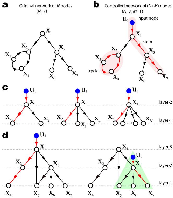
Figure 1: Control centrality. (a) A simple network of $N=7$ nodes. (b) The controlled network is represented by a directed graph $G({\bf A},{\bf B})$ with an input node $u_{1}$ connecting to a state node $x_{1}$. The stem-cycle disjoint subgraph $G_{\mathrm{s}}$ (shown in red) contains six edges, which is the largest number of edges among all possible stem-cycle disjoint subgraphs of the directed graph $G({\bf A},{\bf B})$ and corresponds to the generic dimension of controllable subspace by controlling node $x_{1}$. The control centrality of node $1$ is thus $C_{\mathrm{c}}(1)=6$. (c) The control centrality of the central hub in a directed star is always 2 for any network size $N\geq 2$. (d) The control centrality of a node in a directed acyclic graph (DAG) equals its layer index. In applying Hosoe’s theorem, if not all state nodes are accessible, we just need to consider the accessible part (highlighted in green) of the input node(s).

The calculation of $\mathrm{rank}_{\mathrm{g}}({\bf C})$ can be mapped into a combinatorial optimization problem on a directed graph $G({\bf A},{\bf B})$ constructed as follows Hosoe (1980). Connect the $M$ input nodes $\{u_{1},\cdots,u_{M}\}$ to the $N$ state nodes $\{x_{1},\cdots,x_{N}\}$ in the original network according to the input matrix ${\bf B}$, i.e. connect $u_{j}$ to $x_{i}$ if $b_{ij}\neq 0$, obtaining a directed graph $G({\bf A},{\bf B})$ with $N+M$ nodes (see Fig. 1a and b). A state node $j$ is called accessible if there is at least one directed path reaching from one of the input nodes to node $j$. In Fig. 1b, all state nodes $\{x_{1},\cdots,x_{7}\}$ are accessible from the input node $u_{1}$. A stem is a directed path starting from an input node, so that no nodes appear more than once in it, e.g. $u_{1}\to x_{1}\to x_{5}\to x_{7}$ in Fig. 1b. Denote with $G_{\mathrm{s}}$ the stem-cycle disjoint subgraph of $G({\bf A},{\bf B})$, such that $G_{\mathrm{s}}$ consists of stems and cycles only, and the stems and cycles have no node in common (highlighted in Fig. 1b). According to Hosoe’s theoremHosoe (1980), the generic dimension of the controllable subspace is given by

$$\mathrm{rank}_{\mathrm{g}}({\bf C})=\max_{G_{\mathrm{s}}\in{\cal G}}{|E(G_{\mathrm{s}})|}$$ (3)

with ${\cal G}$ the set of all stem-cycle disjoint subgraphs of the accessible part of $G({\bf A},{\bf B})$ and $|E(G_{\mathrm{s}})|$ the number of edges in the subgraph $G_{\mathrm{s}}$. For example, the subgraph highlighted in Fig. 1b, denoted as $G_{\mathrm{s}}^{\mathrm{max}}$, contains the largest number of edges among all possible stem-cycle disjoint subgraphs. Thus, $C_{\mathrm{c}}(1)=\mathrm{rank}_{\mathrm{g}}({\bf C}^{(1)})=6$, which is the number of red links in Fig. 1b. Note that $\mathrm{rank}_{\mathrm{g}}({\bf C}^{(1)})=6<N=7$, the whole system is therefore not structurally controllable by controlling $x_{1}$ only. Yet, the nodes covered by the $G_{\mathrm{s}}^{\mathrm{max}}$ highlighted in Fig. 1b, e.g. $\{x_{1},x_{2},x_{3},x_{4},x_{5},x_{7}\}$, constitute a structurally controllable subsystem Blackhall and Hill (2010). In other words, by controlling node $x_{1}$ with a time dependent signal $u_{1}(t)$ we can drive the subsystem $\{x_{1},x_{2},x_{3},x_{4},x_{5},x_{7}\}$ from any initial state to any final state in finite time, for almost all sets of values of the free parameters of ${\bf A}$ and ${\bf B}$ except an exceptional set of values with zero measure. In general $G_{\mathrm{s}}^{\mathrm{max}}$ is not unique. For example, in Fig. 1b we can get the same cycle $x_{2}\to x_{3}\to x_{4}\to x_{2}$ together with a different stem $u_{1}\to x_{1}\to x_{5}\to x_{6}$, which yield a different $G_{\mathrm{s}}^{\mathrm{max}}$ and thus a different structurally controllable subsystem $\{x_{1},x_{2},x_{3},x_{4},x_{5},x_{6}\}$. Both subsystems are of size six, which is exactly the generic dimension of the controllable subspace. Note that we can fully control each subsystem individually, yet we cannot fully control the whole system.

The advantage of Eq.(3) is that $\max_{G_{\mathrm{s}}\in{\cal G}}{|E(G)|}$ can be calculated via linear programming Poljak (1990), providing us an efficient numerical tool to determine the control centrality and the structurally controllable subsystem of any node in an arbitrary complex network (see Supplementary Material Sec.I.A).

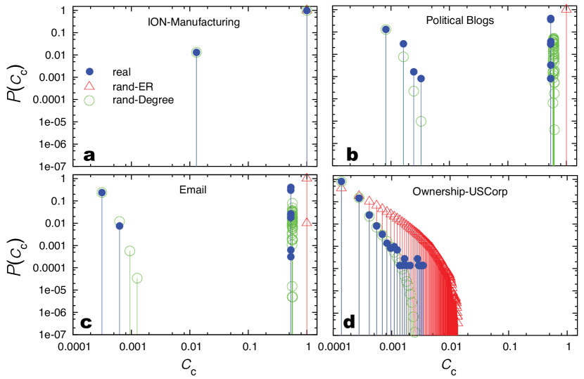
Figure 2: Distribution of normalized control centrality of several real-world networks (blue) and their randomized counterparts: rand-ER (red), rand-Degree (green). (a) Intra-organizational network of a manufacturing company Cross and Parker (2004). (b) Hyperlinks between weblogs on US politics Adamic and Glance . (c) Email network in a university Eckmann et al. (2004). (d) Ownership network of US corporations Norlen et al. .

We first consider the distribution of control centrality. Shown in Fig. 2 is the distribution of the normalized control centrality ($c_{\mathrm{c}}(i)\equiv C_{\mathrm{c}}(i)/N$) for several real networks. We find that for the intra-organization network, $P(c_{\mathrm{c}})$ has a sharp peak at $c_{\mathrm{c}}=1$, suggesting that a high fraction of nodes can individually exert full control over the whole system (Fig. 2a). In contrast, for company-ownership network, $P(c_{\mathrm{c}})$ follows an approximately exponential distribution (Fig. 2d), indicating that most nodes display low control centrality. Even the most powerful node, with $c_{\mathrm{c}}\sim 0.01$, can control only one percent of the total dimension of the system’s full state space. For other networks $P(c_{\mathrm{c}})$ displays a mixed behavior, indicating the coexistence of a few powerful nodes with a large number of nodes that have little control over the system’s dynamics (Fig. 2b,c). Note that under full randomization, turning a network into a directed Erdős-Rényi (ER) random network Erdős and Rényi (1960); Bollobás (2001) with number of nodes ($N$) and number of edges ($L$) unchanged, the $c_{\mathrm{c}}$ distribution changes dramatically. In contrast, under degree-preserving randomization  Maslov and Sneppen (2002); Milo et al. (2002), which keeps the in-degree ($k_{\mathrm{in}}$) and out-degree ($k_{\mathrm{out}}$) of each node unchanged, the $c_{\mathrm{c}}$ distribution does not change significantly. This result suggests that $P(c_{\mathrm{c}})$ is mainly determined by the underlying network’s degree distribution $P(k_{\mathrm{in}},k_{\mathrm{out}})$. This result is very useful in the following sense: $P(k_{\mathrm{in}},k_{\mathrm{out}})$ is easy to calculate for any complex network, while the calculation of $P(c_{\mathrm{c}})$ requires much more computational efforts (both CPU time and memory space). Studying $P(c_{\mathrm{c}})$ for model networks of prescribed $P(k_{\mathrm{in}},k_{\mathrm{out}})$ will give us qualitative understanding of how $P(c_{\mathrm{c}})$ changes as we vary network parameters, e.g. mean degree $\langle k\rangle$. See Supplementary Material Sec.II for more details.

To understand which topological features determine the control centrality itself, we compared the control centrality for each node in the real networks and their randomized counterparts (denoted as rand-ER and rand-Degree). The lack of correlations indicates that both randomization procedures eliminate the topological feature that determines the control centrality of a given node (see Supplementary Material Sec.I.B). Since accessibility plays an important role in maintaining structural controllability Lin (1974), we conjecture that the control centrality of node $i$ is correlated with the number of nodes $N_{\mathrm{r}}(i)$ that can be reached from it. To test this conjecture, we calculated $N_{\mathrm{r}}(i)$ and $C_{\mathrm{c}}(i)$ for the real networks shown in Fig. 2, observing only a weak correlation between the two quantities (see Supplementary Material Sec.I.C). This lack of correlation between $N_{\mathrm{r}}(i)$ and $C_{\mathrm{c}}(i)$ is obvious in a directed star, in which a central hub ($x_{1}$) points to $N-1$ leaf nodes ($x_{2},\cdots,x_{N}$) (Fig. 1c). As the central hub can reach all nodes, $N_{\mathrm{r}}(1)=N$, suggesting that it should have high control centrality. Yet, one can easily check that the central hub has control centrality $C_{\mathrm{c}}(1)=2$ for any $N\geq 2$ and there are $N-1$ structurally controllable subsystems, i.e. $\{x_{1},x_{2}\},\cdots,\{x_{1},x_{N-1}\}$. In other words, by controlling the central hub we can fully control each leaf node individually, but we cannot control them collectively.

Note that in a directed star each node can be labeled with a unique layer index: the leaf nodes are in the first layer (bottom layer) and the central hub is in the second layer (top layer). In this case the control centrality of the central hub equals its layer index (see Fig. 1c). This is not by coincidence: we can prove that for a directed network containing no cycles, often called a directed acyclic graph (DAG), the control centrality of any node equals its layer index

$$C_{\mathrm{c}}(i)=l_{i}.$$ (4)

Indeed, lacking cycles, a DAG has a unique hierarchical structure, which means that each node can be labeled with a unique layer index ($l_{i}$), calculated using a recursive labeling algorithm Yan et al. (2010): (1) Nodes that have no outgoing links ($k_{\mathrm{out}}=0$) are labeled with layer index 1 (bottom layer). (2) Remove all nodes in layer 1. For the remaining graph identify again all nodes with $k_{\mathrm{out}}=0$ and label them with layer index 2. (3) Repeat step (2) until all nodes are labeled. As the DAG lacks cycles, each subgraph in the set ${\cal G}$ of the directed graph $G({\bf A},{\bf b}^{(i)})$ consists of a stem only, which starts from the input node pointing to the state node $i$ and ends at a state node in the bottom layer, e.g. $u_{1}\to x_{1}\to x_{2}\to x_{4}$ in Fig. 1d. The number of edges in this stem is equal to the layer index of node $i$, so $\mathrm{rank}_{\mathrm{g}}({\bf C}^{(i)})=C_{\mathrm{c}}(i)=l_{i}$. Therefore in DAG the higher a node is in the hierarchy, the higher is its ability to control the system. Though this result agrees with our intuition to some extent, it is surprising at the first glance because it indicates that in a DAG the control centrality of node $i$ is only determined by its topological position in the hierarchical structure, rather than any other importance measures, e.g. degree or betweenness centrality. This result also partially explains why driver nodes tend to avoid hubs Liu et al. (2011a).

Despite the simplicity of Eq. (4), we cannot apply it directly to real networks, because most of them are not DAGs. Yet, we note that any directed network has a underlying DAG structure based on the strongly connected component (SCC) decomposition (see Supplementary Material Sec.I.D Fig. S4). A subgraph of a directed network is strongly connected if there is a directed path from each node in the subgraph to every other node. The SCCs of a directed network $G$ are its maximal strongly connected subgraphs. If we contract each SCC to a single supernode, the resulting graph $\widetilde{G}$, called the condensation of $G$, is a DAG Harary (1994). Since a DAG has a unique hierarchical structure, a directed network can then be assigned an underlying hierarchical structure. The layer index of node $i$ can be defined to be the layer index of the corresponding supernode (i.e. the SCC that node $i$ belongs to) in $\widetilde{G}$. With this definition of $l_{i}$, it is easy to show that $C_{\mathrm{c}}(i)\geq l_{i}$ for general directed networks. Furthermore, for an edge $(i\to j)$ in a general directed network, if node $i$ is topologically “higher” than node $j$ (i.e. $l_{i}>l_{j}$), then $C_{\mathrm{c}}(i)>C_{\mathrm{c}}(j)$. Since $C_{\mathrm{c}}(i)$ has to be calculated via linear programming which is computationally more challenging than the calculation of $l_{i}$, the above results suggest an efficient way to calculate the lower bound of $C_{\mathrm{c}}(i)$ and to compare the control centralities of two neighboring nodes. Note that if $l_{i}>l_{j}$ and there is no directed edge $(i\to j)$ in the network, then in general one cannot conclude that $C_{\mathrm{c}}(i)>C_{\mathrm{c}}(j)$ (see Supplementary Material Sec.I.D for more details).

Our finding on the relation between control centrality and hierarchical structure inspires us to design an efficient attack strategy against malicious networks, aiming to affect their controllability. The most efficient way to damage the controllability of a network is to remove all input nodes $\{u_{1},u_{2},\cdots,u_{M}\}$, rendering the system completely uncontrollable. But this requires a detailed knowledge of the control configuration, i.e. the wiring diagram of $G({\bf A},{\bf B})$, which we often lack. If the network structure (${\bf A}$) is known, one can attempt a targeted attack, i.e. rank the nodes according to some centrality measure, like degree or control centrality, and remove the nodes with highest centralities Albert et al. (2000); Cohen et al. (2003). Though we still lack systematic studies on the effect of a targeted attack on a network’s controllability, one naively expects that this should be the most efficient strategy. But we often lack the knowledge of the network structure, which makes this approach unfeasible anyway. In this case a simple strategy would be random attack, i.e. remove a randomly chosen $P$ fraction of nodes, which naturally serves as a benchmark for any other strategy. Here we propose instead a random upstream attack strategy: randomly choose a $P$ fraction of nodes, and for each node remove one of its incoming or upstream neighbors if it has one, otherwise remove the node itself. A random downstream attack can be defined similarly, removing the node to which the chosen node points to. In undirected networks, a similar strategy has been proposed for efficient immunization Cohen et al. (2003) and the early detection of contagious outbreaks Christakis and Fowler (2010), relying on the statistical trend that randomly selected neighbors have more links than the node itself Feld (1991); Newman (2003). In directed networks we can prove that randomly selected upstream (or downstream) neighbors have more outgoing (or incoming) links than the node itself (see Supplementary Material Sec.III.A). Thus a random upstream (or downstream) attack will remove more hubs and more links than the random attack does. But the real reason why we expect a random upstream attack to be efficient in a directed network is because $C_{\mathrm{c}}(i)\geq C_{\mathrm{c}}(j)$ for most edges $(i\to j)$, i.e. the control centrality of the starting node is usually no less than the ending node of a directed edge. In DAGs, for any edge $(i\to j)$, we have strictly $C_{\mathrm{c}}(i)>C_{\mathrm{c}}(j)$ (see Supplementary Material Sec.III.B). Thus, the upstream neighbor of a node is expected to play a more important or equal role in control than the node itself, a result deeply rooted in the nature of the control problem, rather than the hub status of the upstream nodes.

To show the efficiency of the random upstream attack we compare its impact on fully controlled networks with several other strategies. We start from a network that is fully controlled ($\mathrm{rank}_{\mathrm{g}}({\bf C})=N$) via a minimum set of $N_{\mathrm{D}}$ driver nodes. After the attack a $P$ faction of nodes are removed, denoting with $\mathrm{rank}_{\mathrm{g}}({\bf C}^{\prime})$ the dimension of the controllable subspace of the damaged network. We calculate $\mathrm{rank}_{\mathrm{g}}({\bf C}^{\prime})$ as a function of $P$, with $P$ tuned from 0 up to 1. Since the random attack serves as a natural benchmark, we calculate the difference of $\mathrm{rank}_{\mathrm{g}}({\bf C}^{\prime})$ between a given strategy and the random attack, denoted as $\delta=[\mathrm{rank}_{\mathrm{g}}^{\mathrm{Strategy}-j}({\bf C}^{\prime})-\mathrm{rank}_{\mathrm{g}}^{\mathrm{Random}}({\bf C}^{\prime})]/N$. Apparently, the more negative is $\delta$, the more efficient is the strategy compared to a fully random attack. We find that for most networks random upstream attack results in $\delta<0$ for $0<P<1$, i.e. it causes more damage to the network’s controllability than random attack (see Fig. 3b,c,d). Moreover, random upstream attack typically is more efficient than random downstream attack, even though in both cases we remove more hubs and more links than in the random attack. This is due to the fact that the upstream (or downstream) neighbors are usually more (or less) “powerful” than the node itself.

The efficiency of the random upstream attack is even comparable to targeted attacks (Fig. 3). Since the former requires only the knowledge of the network’s local structure rather than any knowledge of the nodes’ centrality measures or any other global information (i.e. the structure of the ${\bf A}$ matrix) while the latter rely heavily on them, this finding indicates the advantage of the random upstream attack. The fact that those targeted attacks do not always show significant superiority over the random attack and the random upstream (downstream) attack could be due to an overlap effect — two targeted nodes successively chosen from the rank list based on some centrality measure are likely to have larger overlap between their controllable subspaces than two randomly chosen nodes. Therefore, successively removing targeted nodes with highest centralities will not always cause the most damage to the network’s controllability. Random attacks can avoid such overlap to some extent because the removed nodes are randomly chosen. This also explains why sometimes targeted attacks are worse than the random attack (see Fig. 3a). Notice that for the intra-organization network all attack strategies fail in the sense that $\delta$ is either positive or very close to zero (Fig. 3a). This is due to the fact this network is so dense ($\langle k\rangle\approx 58$) that we have $C_{\mathrm{c}}(i)=C_{\mathrm{c}}(j)=N$ for almost all the edges $(i\to j)$. Consequently, both random upstream and downstream attacks are not efficient and the $C_{\mathrm{c}}$-targeted attack shows almost the same impact as the random attack. This result suggests that when the network becomes very dense its controllability becomes extremely robust against all kinds of attacks, consistent with our previous result on the core percolation and the control robustness against link removal Liu et al. (2011a). We also tested those attack strategies on model networks (see Supplementary Material Sec.III.C). The results are qualitatively consistent with what we observed in real networks.

In sum, we study the control centrality of single node in complex networks and find that it is related to the underlying hierarchical structure of networks. The presented results help us better understand the controllability of complex networks and design an efficient attack strategy against network control. This work was supported by the Network Science Collaborative Technology Alliance sponsored by the US Army Research Laboratory under Agreement Number W911NF-09-2-0053; the Office of Naval Research under Agreement Number N000141010968; the Defense Threat Reduction Agency awards WMD BRBAA07-J-2-0035 and BRBAA08-Per4-C-2-0033; and the James S. McDonnell Foundation 21st Century Initiative in Studying Complex Systems.

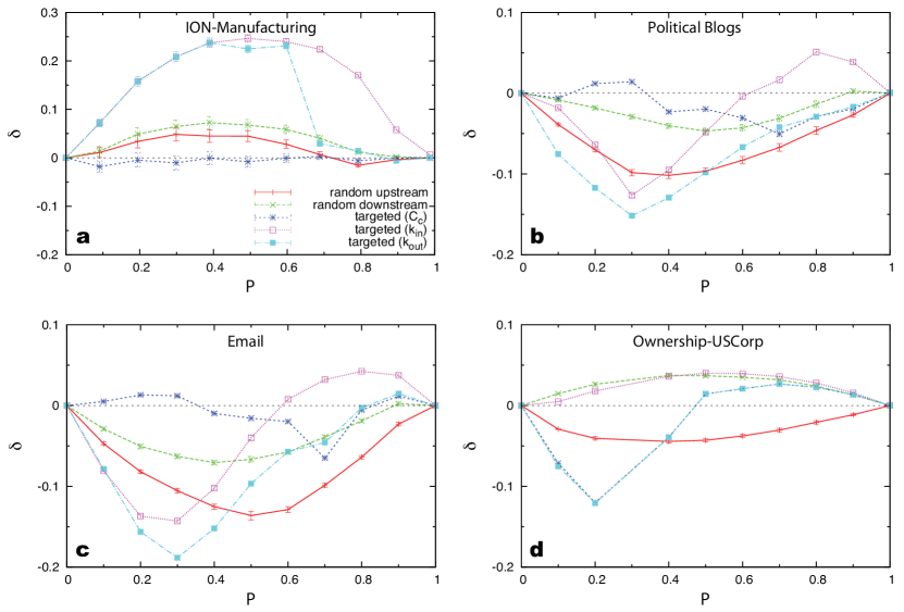
Figure 3: The impact of different attack strategies on network controllability with respective to the random attack. $\delta\equiv[\mathrm{rank}_{\mathrm{g}}^{\mathrm{Strategy}-j}({\bf C}^{\prime})-\mathrm{rank}_{\mathrm{g}}^{\mathrm{Random}}({\bf C}^{\prime})]/N$ with $\mathrm{rank}_{\mathrm{g}}^{\mathrm{Strategy}-j}({\bf C}^{\prime})$ represents the generic dimension of controllable subspace after removing a $P$ fraction of nodes using strategy-$j$. The nodes are removed according to six different strategies. (Strategy-0) Random attack: randomly remove $P$ fraction of nodes. (Strategy-1 or 2) Random upstream (or downstream) attack: randomly choose $P$ fraction of nodes, randomly remove one of their upstream neighbors (or downstream neighbors). The results are averaged over 10 random choices of $P$ fraction of nodes with error bars defined as s.e.m. Lines are only a guide to the eye. (Strategy-3,4, or 5) Targeted attacks: remove the top $P$ fraction of nodes according to their control centralities (or in-degrees or out-degrees).

References

- Albert and Barabási (2002) R. Albert and A.-L. Barabási, Rev. Mod. Phys. 74, 47 (2002).
- Newman et al. (2006) M. Newman, A.-L. Barabási, and D. J. Watts, The Structure and Dynamics of Networks (Princeton University Press, Princeton, 2006).
- Barabási and Albert (1999) A.-L. Barabási and R. Albert, Science 286, 509 (1999).
- Watts and Strogatz (1998) D. J. Watts and S. H. Strogatz, Nature 393, 440 (1998).
- Wang and Chen (2002) X. F. Wang and G. Chen, Physica A 310, 521 (2002).
- Tanner (2004) H. G. Tanner, Decision and Control, 2004. CDC. 43rd IEEE Conference on 3, 2467 (2004).
- Sorrentino et al. (2007) F. Sorrentino, M. di Bernardo, F. Garofalo, and G. Chen, Phys. Rev. E 75, 046103 (2007).
- Yu et al. (2009) W. Yu, G. Chen, and J. Lü, Automatica 45, 429 (2009).
- Lombardi and Hörnquist (2007) A. Lombardi and M. Hörnquist, Phys. Rev. E 75, 056110 (2007).
- Rahmani et al. (2009) A. Rahmani, M. Ji, M. Mesbahi, and M. Egerstedt, SIAM J. Control Optim. 48, 162 (2009).
- Mesbahi and Egerstedt (2010) M. Mesbahi and M. Egerstedt, Graph Theoretic Methods in Multiagent Networks (Princeton University Press, Princeton, 2010).
- Liu et al. (2011a) Y.-Y. Liu, J.-J. Slotine, and A.-L. Barabási, Nature 473, 167 (2011a).
- Liu et al. (2011b) Y.-Y. Liu, J.-J. Slotine, and A.-L. Barabási, Nature 478, E4 (2011b).
- Egerstedt (2011) M. Egerstedt, Nature 473, 158 (2011), 10.1038/473158a.
- Nepusz and Vicsek (2011) T. Nepusz and T. Vicsek, arXiv:1112.5945v1 (2011).
- Cowan et al. (2011) N. J. Cowan, E. J. Chastain, D. A. Vilhena, J. S. Freudenberg, and C. T. Bergstrom, arXiv:1106.2573v3 (2011).
- Wang et al. (2012) W.-X. Wang, X. Ni, Y.-C. Lai, and C. Grebogi, Physical Review E 85, 1 (2012).
- Kalman (1963) R. E. Kalman, J. Soc. Indus. and Appl. Math. Ser. A 1, 152 (1963).
- Luenberger (1979) D. G. Luenberger, Introduction to Dynamic Systems: Theory, Models, & Applications (John Wiley & Sons, New York, 1979).
- Slotine and Li (1991) J.-J. Slotine and W. Li, Applied Nonlinear Control (Prentice-Hall, 1991).
- Lin (1974) C.-T. Lin, IEEE Trans. Auto. Contr. 19, 201 (1974).
- Shields and Pearson (1976) R. W. Shields and J. B. Pearson, IEEE Trans. Auto. Contr. 21, 203 (1976).
- Hosoe (1980) S. Hosoe, IEEE Trans. Auto. Contr. 25, 1192 (1980).
- Dion et al. (2003) J.-M. Dion, C. Commault, and J. van der Woude, Automatica 39, 1125 (2003), ISSN 0005-1098.
- Blackhall and Hill (2010) L. Blackhall and D. J. Hill, in 2nd IFAC Workshop on Distributed Estimation and Control in Networked Systems (2010), pp. 245–250.
- Poljak (1990) S. Poljak, IEEE Trans. Auto. Contr. 35, 367 (1990).
- Erdős and Rényi (1960) P. Erdős and A. Rényi, Publ. Math. Inst. Hung. Acad. Sci. 5, 17 (1960).
- Bollobás (2001) B. Bollobás, Random Graphs (Cambridge University Press, Cambridge, 2001).
- Maslov and Sneppen (2002) S. Maslov and K. Sneppen, Science 296, 910 (2002).
- Milo et al. (2002) R. Milo, S. Shen-Orr, S. Itzkovitz, N. Kashtan, D. Chklovskii, and U. Alon, Science 298, 824 (2002).
- Yan et al. (2010) K.-K. Yan, G. Fang, N. Bhardwaj, R. P. Alexander, and M. Gerstein, Proc. Natl. Acad. Sci. USA (2010).
- Harary (1994) F. Harary, Graph Theory (Westview Press, 1994).
- Albert et al. (2000) R. Albert, H. Jeong, and A.-L. Barabási, Nature 406, 378 (2000).
- Cohen et al. (2003) R. Cohen, S. Havlin, and D. ben Avraham, Phys. Rev. Lett. 91, 247901 (2003).
- Christakis and Fowler (2010) N. A. Christakis and J. H. Fowler, PLoS ONE 5, e12948 (2010).
- Feld (1991) S. L. Feld, Am. J. Soc. 96, 1464 (1991).
- Newman (2003) M. E. J. Newman, Soc. Netw. 25, 83 (2003).
- Cross and Parker (2004) R. Cross and A. Parker, The Hidden Power of Social Networks (Harvard Business School Press, Boston, MA, 2004).
- (39) L. A. Adamic and N. Glance, The political blogosphere and the 2004 us election, Proceedings of the WWW-2005 Workshop on the Weblogging Ecosystem (2005).
- Eckmann et al. (2004) J.-P. Eckmann, E. Moses, and D. Sergi, Proc. Natl. Acad. Sci. USA 101, 14333 (2004).
- (41) K. Norlen, G. Lucas, M. Gebbie, and J. Chuang, Eva: Extraction, visualization and analysis of the telecommunications and media ownership network, Proceedings of International Telecommunications Society 14th Biennial Conference,Seoul Korea (2002).