The Importance of Broad Emission-Line Widths in Single Epoch Black Hole Mass Estimates

Abstract

Estimates of the mass of super-massive black holes (BHs) in distant active galactic nuclei (AGNs) can be obtained efficiently only through single-epoch spectra, using a combination of their broad emission-line widths and continuum luminosities. Yet the reliability and accuracy of the method, and the resulting mass estimates, $M_{\rm BH}$, remain uncertain. A recent study by Croom using a sample of SDSS, 2QZ and 2SLAQ quasars suggests that line widths contribute little information about the BH mass in these single-epoch estimates and can be replaced by a constant value without significant loss of accuracy. In this Letter, we use a sample of nearby reverberation-mapped AGNs to show that this conclusion is not universally applicable. We use the bulge luminosity ($L_{\rm Bulge}$) of these local objects to test how well the known $M_{\rm BH}-L_{\rm Bulge}$ correlation is recovered when using randomly assigned line widths instead of the measured ones to estimate $M_{\rm BH}$. We find that line widths provide significant information about $M_{\rm BH}$, and that for this sample, the line width information is just as significant as that provided by the continuum luminosities. We discuss the effects of observational biases upon the analysis of Croom and suggest that the results can probably be explained as a bias of flux-limited, shallow quasar samples.

1 Introduction

Super-massive black holes (BHs) at the center of galaxies are believed to play a fundamental role in the evolution of galaxies. Accreting BHs, or active galactic nuclei (AGNs), are thought, for example, to be responsible for the quenching of star-formation in galaxies needed to explain the existence of the blue cloud and the red sequence (e.g., Granato et al., 2004; Di Matteo et al., 2005; Hopkins et al., 2005) and for heating gas near the centers of galaxy clusters to stop gas accretion onto the central galaxies (e.g., Croton et al., 2006). This makes characterizing the masses and accretion rates of the BH population across cosmic time crucial to understanding the evolution of galaxies and clusters.

Direct dynamical measurements of the mass of BHs are, however, possible only for nearby quiescent galaxies using spatially resolved velocity measurements inside (or close to) the black hole’s sphere of influence (e.g., Merritt & Ferrarese, 2001; Gültekin et al., 2009). Fortunately, AGNs provide a completely different means of directly estimating $M_{\rm BH}$ through reverberation mapping (RM; Blandford & McKee, 1982; Peterson, 1993). Here it is assumed that the gas responsible for the broad-line emission is virialized and that the broad-line velocity widths are related to the orbital speed of the gas around the black hole. Estimates of $M_{\rm BH}$ are then obtained by combining the width of the emission lines with an estimate of the distance from the BH to the broad line region ($R_{\rm BLR}$). Since AGNs are typically variable, $R_{\rm BLR}$ is estimated using the time it takes for the broad-emission lines to respond to changes in the accretion disk luminosity.

While the RM technique can in principle be used for sources at any distance, it is time consuming, and has been impractical for luminous and distant objects whose variability timescales are long due to their high luminosity (e.g., Vanden Berk et al., 2004; MacLeod et al., 2010) and time dilation. Local RM observations have, however, shown that $R_{\rm BLR}$ is tightly correlated with the luminosity of the accretion disk (e.g., Kaspi et al., 2000; Bentz et al., 2009b). This allows one to estimate $R_{\rm BLR}$ directly from the luminosity, and hence estimate $M_{\rm BH}$ from the single-epoch (SE) spectra used to determine the line widths. In practice, SE $M_{\rm BH}$ estimates are obtained by means of

$$M_{\rm BH}\ =\ f\ \frac{(\Delta v)^{2}\ L_{\lambda}^{\alpha}}{G}$$ (1)

where $\Delta v$ is the velocity width of a given broad emission line, $L_{\lambda}$ is the luminosity of the continuum at an associated wavelength $\lambda$ (in Å), $\alpha\approx 1/2$ but may depend weakly on $\lambda$, $G$ is the gravitational constant and $f$ is a dimensionless factor that accounts for the geometry and inclination of the BLR and the characterization of the line width used in defining the relation. The two most common line-width characterizations are the full-width at half maximum (FWHM) and the line dispersion ($\sigma_{l}$; see, e.g., Peterson et al., 2004). The most common combinations of broad lines and continuum luminosities used are H$\beta$ and $L_{5100}$ ($\alpha=0.519$, Bentz et al., 2009b) at low redshift, and Mg ii with $L_{3000}$ ($\alpha=0.47$, McLure & Jarvis, 2002) or C iv with $L_{1350}$ ($\alpha=0.53$, Vestergaard & Peterson, 2006) at higher redshifts, where these lines appear at observed-frame optical wavelengths.

Recently, Croom (2011, hereafter C11) used a large sample of quasars from the Sloan Digital Sky Survey (SDSS, York et al., 2000), the 2dF QSO Redshift Survey (2QZ, Croom et al., 2004) and the 2dF-SDSS LRG and QSO Survey (2SLAQ, Richards et al., 2005) to study the importance of line-width estimates for the accuracy of SE $M_{\rm BH}$ estimates. For each of the H$\beta$, Mg ii, and C iv lines, C11 observed that the distributions of SE $M_{\rm BH}$ estimates were not significantly different before and after scrambling the line widths across the sample. C11 also noted that the distribution of line widths with redshift was relatively narrow and showed little evolution with redshift. C11 concluded that line widths provide little additional information about BH masses as required by equation (1) compared to simply using a constant value.

While this is a very interesting observation, it conflates three possible explanations: i) that the underlying assumptions behind equation (1) are not correct and that $\Delta v$ truly holds no physical information, ii) that for the typically low $S/N$ spectra used, estimates of $\Delta v$ are so noisy that their physical information is lost or biased, and iii) that due to a conspiracy between the survey selection function and the evolution of the quasar mass, luminosity and accretion rate distributions, the observed distribution of $\Delta v$ is narrow and non-evolving with redshift, minimizing the effects of its randomization on $M_{\rm BH}$. In this Letter, we try to separate these issues. First, in §2, we consider the local, reverberation-mapped sample, where independent indirect estimates of $M_{\rm BH}$ are possible through the well-known correlation with the luminosity of the spheroidal component of the host galaxy. Using this sample, we show that the velocities provide almost as much information on $M_{\rm BH}$ as the luminosities. Then, in §3 we discuss the effects of observational biases on the conclusions of C11. Where needed, we assume a $\Lambda$CDM flat cosmology with $H_{0}=73~{}\rm km~{}\rm s^{-1}~{}\rm Mpc^{-1}$, $\Omega_{\Lambda}=0.7$ and $\Omega_{M}=0.3$.

2 Are Line Widths Important for Accurate BH Mass Estimates?

In order to understand the importance of line widths in SE $M_{\rm BH}$ estimates, we use a sample of 34 nearby AGNs observed in reverberation mapping (RM) campaigns with bulge luminosity measurements at 5100Å, $L_{\rm Bulge}$, by Bentz et al. (2009a) using HST. Although the target selection is somewhat arbitrary, the sample is approximately volume limited, as luminous, distant sources are generally avoided in RM studies due to cosmological time-dilation and their intrinsically longer variability timescales. The inherent difficulty in measuring bulge luminosities of distant AGNs further constrains the sample distance. The sample properties are summarized in Table 1.

Every object in our sample has been the subject of at least one RM observational campaign, and many for two or more. For each object we use the mean optical spectrum of each reverberation mapping campaign, and we treat each of the 62 mean spectra as independent objects. While there is typically not enough variability from a single object within an RM campaign to treat each individual spectrum as an independent data point, it is a good approximation to assume each observational campaign provides an independent measurement. Although for any one object the dynamic range in luminosity is limited, Peterson et al. (2004) and Bentz et al. (2010) show that RM $M_{\rm BH}$ estimates of NGC 5548, the most studied source, are consistent between campaigns ($\Delta\log{M_{\rm BH}}\approx 0.14~{}\rm dex$). Table 1 also lists the number of individual spectra used to build each mean spectrum.

The host-corrected AGN continuum luminosities at 5100Å, $L_{5100}$, are taken from Bentz et al. (2009a), while the broad H$\beta$ FWHM and $\sigma_{l}$ measurements are taken directly from the references listed in Table 1. While this leads to some heterogeneity in the recipes used to make the line-width measurements, the (typically) extremely high $S/N$ of the mean spectra minimizes the resulting systematic errors (Denney et al., 2009a). The distributions of the sample in H$\beta$ FWHM, continuum $L_{5100}$, bulge $L_{\rm Bulge}$, and estimated black hole mass are shown in Figure 1.

The ideal test to determine whether the velocity widths hold information about the BH mass would compare these single-epoch mass estimates to dynamical $M_{\rm BH}$ measurements for the same objects. Unfortunately, few AGNs exist with dynamical measurements of $M_{\rm BH}$, rendering such a test infeasible at present. Studies of quiescent galaxies, however, have determined that there is a strong correlation between the mass of the central BH and the luminosity of the spheroidal component of its host galaxy (e.g., Marconi & Hunt, 2003; Graham, 2007, 2012). So while we lack dynamical estimates of $M_{\rm BH}$ for comparison, we can assess the reliability of SE $M_{\rm BH}$ estimates simply by using $L_{\rm Bulge}$ as a proxy and studying how well they hold to the $M_{\rm BH}-L_{\rm Bulge}$ correlation.

We estimate SE BH masses for each object by means of equation (1), using the mean continuum luminosity at 5100Å and either the FWHM or the $\sigma_{l}$ line width characterization of the mean H$\beta$ spectrum. We evaluate the correlation strength between $M_{\rm BH}$ and $L_{\rm Bulge}$ using the Spearman rank-order coefficient, $r_{s}$, finding a value of $r_{s}^{0}=0.69~{}(0.63)$ when using the FWHM ($\sigma_{l}$) for the mass estimates. Given the number of data points, the probability of obtaining such a value of $r_{s}^{0}$ in the absence of a correlation is $P_{\rm Ran}=7.4\times 10^{-10}~{}(5.4\times 10^{-8})$. As expected, our SE $M_{\rm BH}$ estimates are very well correlated with the luminosity of the spheroidal component of their host, suggesting these SE estimates can be quite accurate.

The amount of information obtained by using accurate line-width estimates can then be tested by re-estimating $r_{s}$ using $M_{\rm BH}$ estimates obtained with randomly selected values for the line widths. In practice, we randomly re-distribute the measured line widths across the objects in our sample 500 times, essentially bootstrap resampling the observed FWHM distribution, estimating $r_{s}$ for each realization. In this procedure we never assign a measurement its true line width, although doing so does not alter our main conclusions. Figure 2 shows the resulting distribution of the $r_{s}$ coefficients compared to the value obtained before modifying the original line widths, $r_{s}^{0}$. We only show the results for the FWHM, as those using $\sigma_{l}$ are very similar. Note that $r_{s}^{0}$ is significantly above the distribution obtained by randomizing the line widths. If we view the values of $r_{s}$ as Gaussian random numbers, the true value is 4.3$\sigma$ from the mean of the random trials. The mean value of $r_{s}=0.309$ ($P_{\rm Ran}=1.5\%$) in the random trials is 8 orders of magnitude less significant than that obtained using the real FWHM estimates. This demonstrates that line widths provide very significant information about $M_{\rm BH}$ and that accurate line-width estimates are crucial for accurate SE $M_{\rm BH}$ estimates in this sample. This is illustrated in the top-right panel of Figure 2, which shows the spread in BH mass ratio obtained by combining all 500 random realizations. The difference in the estimated $M_{\rm BH}$ is strongly peaked but also with broad wings, with a standard deviation of 0.65 dex. We find similar results if we include each source only once.

Using the same formalism, we can also investigate the importance of the continuum luminosity for SE $M_{\rm BH}$ estimates by randomizing the continuum luminosities rather than the line-width estimates. The resulting $r_{s}$ distribution is also shown in Figure 2, and it looks very similar to that obtained by randomizing the line widths. This is not surprising, as in our sample the $\sim$2 dex dynamic range in $L_{\rm 5100}^{1/2}$ is similar to that of $\rm FWHM^{2}$ (see Fig. 1). The mean Spearman Rank-order coefficient of the randomized distributions is $r_{s}=0.293$ ($P_{\rm Ran}=2.1\%$) so, for this sample, accurate line widths are just as important as accurate luminosities for SE $M_{\rm BH}$ estimates. Finally, as a cross-check, one can also estimate the probability that the $M_{\rm BH}-L_{\rm Bulge}$ correlation could randomly arise in our sample. We randomize the sample in both $L_{5100}$ and the FWHM, and, as expected, we find an $r_{s}$ distribution consistent with no correlation. The mean of the distribution is $r_{s}=-1.7\times 10^{-3}$, implying $P_{\rm Ran}=99\%$.

3 Discussion

Unless the results of the previous section are not applicable at higher redshift, which is physically implausible, we must now look into the possibility that C11’s results are either due to the low $S/N$ of the spectra or a conspiracy between the surveys and the shape and evolution of both the QSO luminosity and Eddington ratio distributions that leaves the observed line widths in a nearly redshift independent distribution. We note that the sample of C11 is overwhelmingly dominated by SDSS observations, accounting for 100%, 71% and 86% of the H$\beta$, Mg ii and C iv measurements, respectively. For simplicity, the following discussion focuses solely on the SDSS data.

Denney et al. (2009a) have shown that H$\beta$ line-width estimates can be significantly in error for low signal-to-noise ratio ($S/N$) spectra, with systematic and random error components that scale with $S/N$. The errors are small for $S/N\sim 20$, but at a typical $S/N\sim 5$, Denney et al. (2009a) observed a shift of 0.10 dex to larger BH masses, and the dispersion increased by 0.12 dex. While in principle this shift could be due to either errors in the line widths or continuum luminosities, $L_{5100}$ is quite insensitive to $S/N$ and $M_{\rm BH}$ only depends on its square root (eqn. [1]). Thus, the errors in $M_{\rm BH}$ found by Denney et al. (2009a) should be dominated by uncertainties in the line-width measurements induced by poor $S/N$.

Given these results, we then consider whether the SDSS data are simply too noisy. We investigated this possibility using a stacking analysis of the SDSS QSO spectra. We use C iv because it has a clean local continuum, and is the line most affected by systematic issues in low $S/N$ spectra (see, e.g., Assef et al., 2011). While this is not ideal, since our discussion and the results of Denney et al. (2009a) have focused solely on H$\beta$, it is still useful since C11 reached identical conclusions for all three of the main QSO broad emission lines used for $M_{\rm BH}$ estimates (H$\beta$, Mg ii and C iv). The details and analysis of these stacked spectra, as well as for Mg ii, are presented by Frank et al. (in prep.). The stacks are produced by averaging approximately 7200 QSO SDSS spectra from the sample of Shen et al. (2008, hereafter S08) in the redshift range $1.857<z<3.118$ and in the small absolute magnitude range $-27.6<M_{i}<-26.6$ mag, divided into 33 bins of FWHM as measured by S08. SDSS quasar redshifts are determined from all possible absorption and emission lines, minimizing the effects of possible C iv blueshifts upon $z$ (see Adelman-McCarthy et al., 2008, for details). In the selection process, known BALQSOs were rejected as they can significantly bias the resulting combined spectra. Before stacking, each individual spectrum is corrected for Galactic reddening using the extinction map of Schlegel et al. (1998), shifted into the rest frame, and normalized by the flux near a rest-frame wavelength of $1700\rm\AA$. The resulting spectra are then continuum subtracted and averaged, and the FWHM is measured directly from the stacked spectra. Our results are qualitatively insensitive to whether we use the median or averaged stacked spectra.

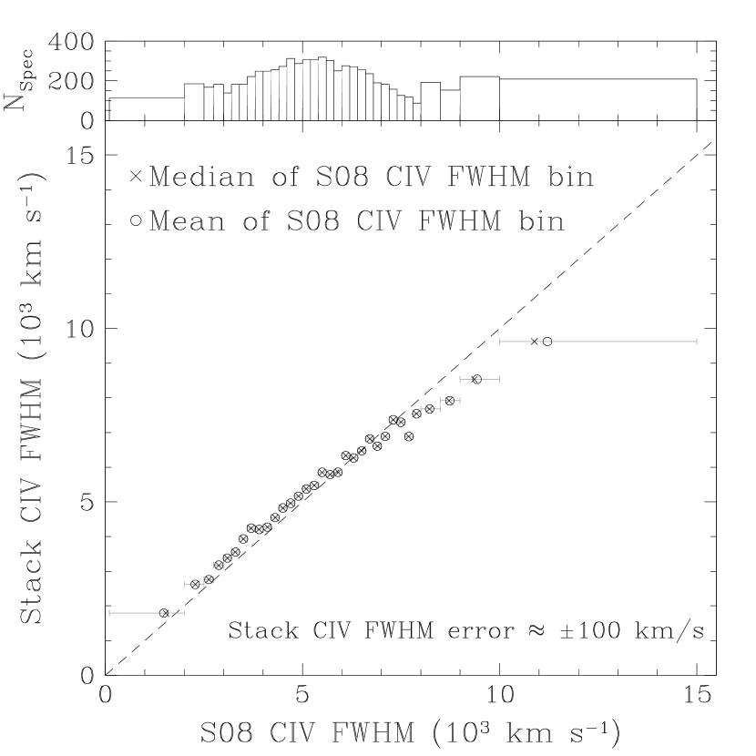
Figure 3: The FWHM of the stacked spectra for each bin of individual S08 FWHM estimates. The open circles (crosses) show the mean (median) of the S08 estimates in each bin. The two estimates agree if on the dashed line. The mean and median are generally almost equal. The horizontal error bars span the range of each S08 FWHM bin. The upper panel shows the number of spectra in each S08 FWHM bin.

Figure 3 compares the FWHM measured from the stacked spectra with the mean and median FWHM estimates of S08 in each bin. We find that the FWHM of the mean spectra agree with the mean/median of the individual estimates. Note, however, that they are moderately biased, particularly at the high velocity end. These issues are explored further by Frank et al. (in prep.). We have also repeated the process for different bins of $M_{i}$, and find qualitatively similar results for all absolute magnitudes. Overall, we consider it is unlikely that the line-width measurements are noisy enough to explain the C11 results, since on average they retain the information of the high $S/N$ stacks, and C iv is the line that is most likely to be affected by systematic biases. Furthermore, we note that C11 uses the inter-percentile value to characterize the line widths for Mg ii and C iv, and these should be more robust at lower $S/N$ than the FWHM.

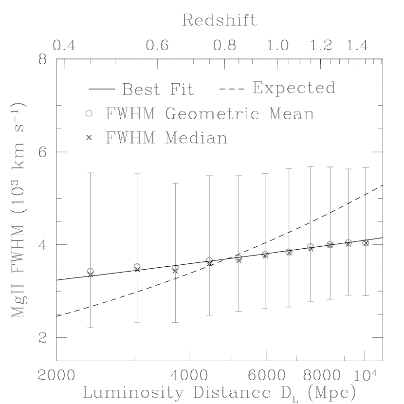
Figure 4: The points show the S08 Mg ii FWHM as a function of redshift. Gray open circles (crosses) show the FWHM geometric mean (median) of the sample in redshift slices of width $\Delta z=0.1$ and the error bars enclose 68.3% of objects above and below the mean. The solid black line shows the best-fit evolution of $\rm FWHM\propto\Gamma(z)^{0.16}$ and the dashed line shows the expected evolution of $\Gamma(z)^{0.5}$ in the absence of $\ell_{Edd}$ evolution, normalized to the observed trend at $D_{L}=5000~{}\rm Mpc$.

Thus, we are left with the conclusion that the narrow and apparently unevolving distribution of line-width measurements in the C11 sample (see his Fig. 1) are caused by a combination of evolution in the Eddington ratio distribution, the quasar luminosity function (QLF) and the SDSS selection function. For example, Figure 4 shows the distribution of Mg ii line widths from S08, selected because they span the broadest range of redshifts. With the simplifying approximation that $\alpha=1/2$ in equation (1), the line width is given by

$$\Delta v\ \propto\ {L^{1/4}\over\ell_{Edd}^{1/2}},$$ (2)

where $\ell_{Edd}$ is the Eddington ratio. We know from Kollmeier et al. (2006) that the $\ell_{Edd}$ distribution of broad-line quasars is narrow. For these bright SDSS AGNs, the steep QLF ($dn/dL\propto L^{-3.1}$ for $z<2.4$, Richards et al., 2006) means that at any given redshift half of quasars are within 0.35 mag of the survey flux limit, corresponding to a velocity spread of only 0.035 dex (8%) if we neglect the narrow width of the $\ell_{Edd}$ distribution. Thus, at fixed redshift we should expect a narrow velocity distribution.

The distribution of $\Delta v$ also shows little evolution with redshift. Note that the luminosity of objects at the flux limit evolves as $L_{min}\propto\Gamma(z)^{2}$, where $\Gamma(z)=D_{L}(z)\ (1+z)^{-0.28}\sim z^{1.07}$ for our cosmology and a mean quasar spectral slope of $f_{\nu}\propto\nu^{-0.44}$ (Vanden Berk et al., 2001). Hence, at fixed $\ell_{Edd}$, the apparent evolution of their associated line widths is $\Delta v\propto\Gamma(z)^{1/2}\sim z^{0.54}$. If we compare this “passive” evolution rate to that observed for Mg ii (Fig. 4), we find that the differences are already surprisingly small. Taken at face value, the difference between the “passive” evolution model and the observed $\rm FWHM\propto\Gamma^{0.16}$ implies an evolution in the Eddington ratio of $\ell_{Edd}\propto\Gamma^{0.68}\sim z^{0.73}$. Hence, the slow evolution of $\Delta v$ may be related to quasar “downsizing” (e.g., Cowie et al., 2003). Whether the slow evolution is due to general changes in the accretion rates with $z$ or evolution in $\ell_{Edd}$ as a function of $M_{\rm BH}$ is a complex problem beyond the scope of this paper. Recent modeling of the QLF and observed $\ell_{Edd}$ distributions by Shankar et al. (2011) suggests that $\ell_{Edd}$ likely evolves in both manners, increasing with increasing $z$ and decreasing $M_{\rm BH}$. That the net result would be to leave almost no apparent evolution is then simply a coincidence. Adding the significant noise in the line-width measurements of low $S/N$ spectra may further blur the signs of a weak evolution with redshift. Since line widths are clearly essential for SE $M_{\rm BH}$ estimates in the local reverberation mapped sample, this seems to be the most natural explanation of the C11 result. We conclude that line widths are as important as continuum luminosities for determining accurate BH masses, but that the evolution of the QSO population likely conspires with the survey flux limit to conceal this in shallow surveys such as SDSS.

Table 1: Reverberation Mapping Sample

Object	$\log L_{5100\AA}$	$\log L_{\rm Bulge}$	FWHM	$\sigma_{l}$	$\rm N_{\rm Spec}$	Ref.
	$\rm erg~{}\rm s^{-1}$	$\rm erg~{}\rm s^{-1}$	$\rm km~{}\rm s^{-1}$	$\rm km~{}\rm s^{-1}$
Mrk335	43.73 $\pm$ 0.05	43.14	01792 $\pm$0003	01380 $\pm$0006	123	1
	43.81 $\pm$ 0.05	43.14	01679 $\pm$0002	01371 $\pm$0008	25	1
PG0026+129	44.95 $\pm$ 0.08	44.36	02544 $\pm$0056	01738 $\pm$0100	53	1
PG0052+251	44.78 $\pm$ 0.09	44.12	05008 $\pm$0073	02167 $\pm$0030	56	1
F9	43.94 $\pm$ 0.06	44.10	05999 $\pm$0060	02347 $\pm$0016	29	1
Mrk590	43.55 $\pm$ 0.05	43.59	02788 $\pm$0029	01942 $\pm$0026	24	1
	43.06 $\pm$ 0.06	43.59	03729 $\pm$0426	02168 $\pm$0030	17	1
	43.33 $\pm$ 0.05	43.59	02743 $\pm$0079	01967 $\pm$0019	16	1
	43.61 $\pm$ 0.08	43.59	02500 $\pm$0043	01880 $\pm$0019	17	1
3C120	44.09 $\pm$ 0.09	43.19	02327 $\pm$0048	01249 $\pm$0021	52	1
Akn120	43.95 $\pm$ 0.04	44.01	06042 $\pm$0035	01753 $\pm$0006	20	1
	43.61 $\pm$ 0.06	44.01	06246 $\pm$0078	01862 $\pm$0013	20	1
Mrk79	43.60 $\pm$ 0.06	43.80	05056 $\pm$0085	02314 $\pm$0023	20	1
	43.71 $\pm$ 0.06	43.80	04760 $\pm$0031	02281 $\pm$0026	19	1
	43.64 $\pm$ 0.06	43.80	04766 $\pm$0071	02312 $\pm$0021	23	1
	43.54 $\pm$ 0.05	43.80	04137 $\pm$0037	01939 $\pm$0016	24	1
PG0804+761	44.88 $\pm$ 0.09	44.18	03053 $\pm$0038	01434 $\pm$0018	70	1
PG0844+349	44.19 $\pm$ 0.06	43.73	02694 $\pm$0058	01505 $\pm$0014	48	1
Mrk110	43.64 $\pm$ 0.06	42.65	01543 $\pm$0005	00962 $\pm$0015	21	1
	43.72 $\pm$ 0.07	42.65	01658 $\pm$0003	00953 $\pm$0010	14	1
	43.49 $\pm$ 0.15	42.65	01600 $\pm$0039	00987 $\pm$0018	28	1
PG0953+414	45.15 $\pm$ 0.07	44.56	03071 $\pm$0027	01659 $\pm$0031	35	1
NGC3227	42.86 $\pm$ 0.08	43.23	04445 $\pm$0134	01914 $\pm$0071	23	1
	42.32 $\pm$ 0.05	43.23	05103 $\pm$0159	02473 $\pm$0026	26	1
	42.11 $\pm$ 0.04	43.23	03972 $\pm$0025	01749 $\pm$0004	75	2
NGC3516	43.17 $\pm$ 0.15	43.77	05236 $\pm$0012	01584 $\pm$0001	74	2
NGC3783	43.02 $\pm$ 0.05	42.86	03770 $\pm$0068	01691 $\pm$0019	73	3
NGC4051	41.88 $\pm$ 0.05	42.86	01453 $\pm$0003	01500 $\pm$0034	29	1
	41.82 $\pm$ 0.03	42.86	00799 $\pm$0002	01045 $\pm$0004	86	4
PG1211+143	44.70 $\pm$ 0.08	43.77	02012 $\pm$0037	01487 $\pm$0030	36	1
PG1226+023	45.93 $\pm$ 0.07	45.05	03509 $\pm$0036	01778 $\pm$0017	39	1
PG1229+204	43.65 $\pm$ 0.06	43.58	03828 $\pm$0054	01608 $\pm$0024	33	1
NGC4593	42.85 $\pm$ 0.04	43.84	05143 $\pm$0016	01790 $\pm$0003	25	5
PG1307+085	44.82 $\pm$ 0.06	44.26	05059 $\pm$0133	01963 $\pm$0047	23	1
IC4329A	42.89 $\pm$ 0.07	44.36	05964 $\pm$0134	02271 $\pm$0058	25	1
Mrk279	43.66 $\pm$ 0.06	43.61	05354 $\pm$0032	01823 $\pm$0011	$<40$	1
PG1411+442	44.52 $\pm$ 0.05	44.08	02801 $\pm$0043	01774 $\pm$0029	24	1
NGC5548	43.35 $\pm$ 0.07	43.93	04674 $\pm$0063	01934 $\pm$0005	132	1
	43.09 $\pm$ 0.07	43.93	05418 $\pm$0107	02227 $\pm$0020	94	1
	43.31 $\pm$ 0.06	43.93	05236 $\pm$0087	02205 $\pm$0016	65	1
	43.02 $\pm$ 0.09	43.93	05986 $\pm$0095	03110 $\pm$0053	83	1
	43.28 $\pm$ 0.06	43.93	05930 $\pm$0042	02486 $\pm$0013	142	1
	43.33 $\pm$ 0.06	43.93	07378 $\pm$0039	02877 $\pm$0017	128	1
	43.48 $\pm$ 0.05	43.93	06946 $\pm$0079	02432 $\pm$0013	78	1
	43.39 $\pm$ 0.08	43.93	06623 $\pm$0093	02276 $\pm$0015	144	1
	43.19 $\pm$ 0.06	43.93	06298 $\pm$0065	02178 $\pm$0012	95	1
	43.55 $\pm$ 0.06	43.93	06177 $\pm$0036	02035 $\pm$0011	119	1
	43.46 $\pm$ 0.08	43.93	06247 $\pm$0057	02021 $\pm$0018	86	1
	43.06 $\pm$ 0.08	43.93	06240 $\pm$0077	02010 $\pm$0030	37	1
	43.06 $\pm$ 0.07	43.93	06478 $\pm$0108	03111 $\pm$0131	45	1
	42.87 $\pm$ 0.05	43.93	06396 $\pm$0167	03210 $\pm$0642	28	6
PG1426+015	44.60 $\pm$ 0.08	44.26	07113 $\pm$0160	02906 $\pm$0080	20	1
Mrk817	43.75 $\pm$ 0.07	42.78	04711 $\pm$0049	01984 $\pm$0008	25	1
	43.63 $\pm$ 0.06	42.78	05237 $\pm$0067	02098 $\pm$0013	17	1
	43.63 $\pm$ 0.05	42.78	04767 $\pm$0072	02195 $\pm$0016	19	1
PG1613+658	44.73 $\pm$ 0.07	44.62	09074 $\pm$0103	03084 $\pm$0033	48	1
PG1617+175	44.36 $\pm$ 0.09	44.11	06641 $\pm$0190	02313 $\pm$0069	34	1
PG1700+518	45.56 $\pm$ 0.05	44.83	02252 $\pm$0085	03160 $\pm$0093	37	1
3C390.3	43.65 $\pm$ 0.08	43.62	12694 $\pm$0013	03744 $\pm$0042	104	1
Mrk509	44.16 $\pm$ 0.09	43.98	03015 $\pm$0002	01555 $\pm$0007	194	1
PG2130+099	44.40 $\pm$ 0.05	42.94	02853 $\pm$0039	01485 $\pm$0015	21	7
NGC7469	43.30 $\pm$ 0.04	44.04	01722 $\pm$0030	01707 $\pm$0020	54	1

Note. — Refs: (1) Peterson et al. (2004) and references therein, (2) Denney et al. (2010), (3) Onken & Peterson (2002), (4) Denney et al. (2009b), (5) Denney et al. (2006), (6) Bentz et al. (2007), (7) Grier et al. (2008). Mean line-widths for the spectra of Peterson et al. (2004) and Onken & Peterson (2002) are presented by Collin et al. (2006).

Figure 1: Distribution of the physical properties of our sample of nearby AGNs. The panels show the distribution of the $L_{5100}$ AGN continuum luminosities (left), broad H$\beta$ FWHM (middle left), SE $M_{\rm BH}$ estimates (middle right) and 5100Å bulge luminosities $L_{\rm Bulge}$ (right).

Figure 2: Panel a) shows the distribution of Spearman rank-order coefficients $r_{s}$ obtained for 500 randomizations of the FWHM measurements across our sample. The dashed line shows the value obtained using the FWHM measurement that corresponds to each object. Panel b shows the distribution of the changes in $M_{\rm BH}$ caused by randomizing the line-widths, i.e., $\Delta\log M_{\rm BH}=\log M_{\rm BH}({\rm FWHM_{\rm Random}})-\log M_{\rm BH}(\rm FWHM_{\rm True})$. The histogram is constructed by combining the logarithmic change in $M_{\rm BH}$ for every object for every realization. Panels c) and d) are analogs to panels a) and b) but after randomizing $L_{5100}$ instead of FWHM.

References

- Adelman-McCarthy et al. (2008) Adelman-McCarthy, J. K., et al. 2008, ApJS, 175, 297
- Assef et al. (2011) Assef, R. J., Denney, K. D., Kochanek, C. S., et al. 2011, ApJ, 742, 93
- Bentz et al. (2009a) Bentz, M. C., Peterson, B. M., Netzer, H., Pogge, R. W., & Vestergaard, M. 2009a, ApJ, 697, 160
- Bentz et al. (2007) Bentz, M. C., et al. 2007, ApJ, 662, 205
- Bentz et al. (2009b) —. 2009b, ApJ, 705, 199
- Bentz et al. (2010) —. 2010, ApJ, 716, 993
- Blandford & McKee (1982) Blandford, R. D., & McKee, C. F. 1982, ApJ, 255, 419
- Collin et al. (2006) Collin, S., Kawaguchi, T., Peterson, B. M., & Vestergaard, M. 2006, A&A, 456, 75
- Cowie et al. (2003) Cowie, L. L., Barger, A. J., Bautz, M. W., Brandt, W. N., & Garmire, G. P. 2003, ApJ, 584, L57
- Croom (2011) Croom, S. M. 2011, ApJ, 736, 161
- Croom et al. (2004) Croom, S. M., Smith, R. J., Boyle, B. J., Shanks, T., Miller, L., Outram, P. J., & Loaring, N. S. 2004, MNRAS, 349, 1397
- Croton et al. (2006) Croton, D. J., et al. 2006, MNRAS, 365, 11
- Denney et al. (2009a) Denney, K. D., Peterson, B. M., Dietrich, M., Vestergaard, M., & Bentz, M. C. 2009a, ApJ, 692, 246
- Denney et al. (2006) Denney, K. D., et al. 2006, ApJ, 653, 152
- Denney et al. (2009b) —. 2009b, ApJ, 702, 1353
- Denney et al. (2010) —. 2010, ApJ, 721, 715
- Di Matteo et al. (2005) Di Matteo, T., Springel, V., & Hernquist, L. 2005, Nature, 433, 604
- Frank et al. (in prep.) Frank, S., et al. in prep.
- Graham (2007) Graham, A. W. 2007, MNRAS, 379, 711
- Graham (2012) —. 2012, ApJ, 746, 113
- Granato et al. (2004) Granato, G. L., De Zotti, G., Silva, L., Bressan, A., & Danese, L. 2004, ApJ, 600, 580
- Grier et al. (2008) Grier, C. J., et al. 2008, ApJ, 688, 837
- Gültekin et al. (2009) Gültekin, K., et al. 2009, ApJ, 698, 198
- Hopkins et al. (2005) Hopkins, P. F., Hernquist, L., Cox, T. J., Di Matteo, T., Martini, P., Robertson, B., & Springel, V. 2005, ApJ, 630, 705
- Kaspi et al. (2000) Kaspi, S., Smith, P. S., Netzer, H., Maoz, D., Jannuzi, B. T., & Giveon, U. 2000, ApJ, 533, 631
- Kollmeier et al. (2006) Kollmeier, J. A., et al. 2006, ApJ, 648, 128
- MacLeod et al. (2010) MacLeod, C. L., et al. 2010, ApJ, 721, 1014
- Marconi & Hunt (2003) Marconi, A., & Hunt, L. K. 2003, ApJ, 589, L21
- McLure & Jarvis (2002) McLure, R. J., & Jarvis, M. J. 2002, MNRAS, 337, 109
- Merritt & Ferrarese (2001) Merritt, D., & Ferrarese, L. 2001, in Astronomical Society of the Pacific Conference Series, Vol. 249, The Central Kiloparsec of Starbursts and AGN: The La Palma Connection, ed. J. H. Knapen, J. E. Beckman, I. Shlosman, & T. J. Mahoney, 335
- Onken & Peterson (2002) Onken, C. A., & Peterson, B. M. 2002, ApJ, 572, 746
- Peterson (1993) Peterson, B. M. 1993, PASP, 105, 247
- Peterson et al. (2004) Peterson, B. M., et al. 2004, ApJ, 613, 682
- Richards et al. (2005) Richards, G. T., et al. 2005, MNRAS, 360, 839
- Richards et al. (2006) —. 2006, AJ, 131, 2766
- Schlegel et al. (1998) Schlegel, D. J., Finkbeiner, D. P., & Davis, M. 1998, ApJ, 500, 525
- Shankar et al. (2011) Shankar, F., Weinberg, D. H., & Miralda-Escude’, J. 2011, ArXiv e-prints
- Shen et al. (2008) Shen, Y., Greene, J. E., Strauss, M. A., Richards, G. T., & Schneider, D. P. 2008, ApJ, 680, 169
- Vanden Berk et al. (2001) Vanden Berk, D. E., et al. 2001, AJ, 122, 549
- Vanden Berk et al. (2004) —. 2004, ApJ, 601, 692
- Vestergaard & Peterson (2006) Vestergaard, M., & Peterson, B. M. 2006, ApJ, 641, 689
- York et al. (2000) York, D. G., et al. 2000, AJ, 120, 1579