On Combining Galaxy Clustering and Weak Lensing to Unveil Galaxy Biasing via the Halo Model

Abstract

We formulate the concept of non-linear and stochastic galaxy biasing in the framework of halo occupation statistics. Using two-point statistics in projection, we define the galaxy bias function, $b_{\rm g}(r_{\rm p})$, and the galaxy-dark matter cross-correlation function, ${\cal R}_{\rm gm}(r_{\rm p})$, where $r_{\rm p}$ is the projected distance. We use the analytical halo model to predict how the scale dependence of $b_{\rm g}$ and ${\cal R}_{\rm gm}$, over the range $0.1h^{-1}\>{\rm Mpc}\lower 3.01385pt\hbox{$\;\buildrel<\over{\sim}\;$}r_{\rm p}\lower 3.01385pt\hbox{$\;\buildrel<\over{\sim}\;$}30h^{-1}\>{\rm Mpc}$, depends on the non-linearity and stochasticity in halo occupation models. In particular we quantify the effect due to the presence of central galaxies, the assumption for the radial distribution of satellite galaxies, the richness of the halo, and the Poisson character of the probability to have a certain number of satellite galaxies in a halo of a certain mass. Overall, brighter galaxies reveal a stronger scale dependence, and out to a larger radius. In real-space, we find that galaxy bias becomes scale independent, with ${\cal R}_{\rm g}=1$, for radii $r\geq 1-5h^{-1}\>{\rm Mpc}$, depending on luminosity. However, galaxy bias is scale-dependent out to much larger radii when one uses the projected quantities defined in this paper. These projected bias functions have the advantage that they are more easily accessible observationally and that their scale dependence carries a wealth of information regarding the properties of galaxy biasing. To observationally constrain the parameters of the halo occupation statistics and to unveil the origin of galaxy biasing we propose the use of the bias function $\Gamma_{\rm gm}(r_{\rm p})\equiv b_{\rm g}(r_{\rm p})/{\cal R}_{\rm gm}(r_{\rm p})$. This function is obtained via a combination of weak gravitational lensing and galaxy clustering, and it can be measured using existing and forthcoming imaging and spectroscopic galaxy surveys.

1 Introduction

According to the current paradigm of structure formation in the Universe, galaxies form and reside within dark matter haloes which emerge from the (non-linear) growth of primordial density fluctuations. In this scenario, one expects that the spatial distribution of galaxies traces, to first order, that of the underlying dark matter. However, due to the complexity of galaxy formation and evolution, galaxies are also expected to be somewhat biased tracers. In general, the relationship between the galaxy and dark matter distribution is loosely referred to as galaxy biasing (see e.g. Davis et al. 1985; Bardeen et al. 1986; Dekel & Rees 1987). At any cosmic epoch, this relation is the end product of processes such as non-linear gravitational collapse, gas cooling, star formation, and possible feedback mechanisms. Therefore, understanding the features of galaxy biasing is crucial for a thorough comprehension of galaxy formation and evolution as well as for the interpretation of those studies which use galaxies as tracers of the underlying dark matter distribution in an attempt to constrain cosmological parameters.

The simplest way to model galaxy biasing is by assuming a linear and deterministic relation between the matter and the galaxy density fields. Galaxy formation, though, is a complicated process and the validity of such a simplistic assumption is highly questionable. As a consequence, numerous authors have presented various arguments for considering modifications from a simple linear and deterministic biasing scheme (e.g., Kaiser 1984; Davis et al. 1985; Bardeen et al. 1986; Dekel & Silk 1986; Dekel & Rees 1987; Braun et al. 1988; Babul & White 1991; Lahav & Saslaw 1992; Scherrer & Weinberg 1998; Tegmark & Peebles 1998; Dekel & Lahav 1999; Taruya & Soda 1999). In addition, cosmological simulations and semi-analytical models of galaxy formation strongly suggest that galaxy bias indeed takes on a non-trivial form (e.g., Cen & Ostriker 1992; Kauffmann et al. 1997; Tegmark & Bromley 1999; Somerville et al. 2001). From the observational side, numerous attempts have been made to test whether galaxy bias is linear and deterministic. This includes studies that compare the clustering properties of different samples of galaxies (e.g., Tegmark & Bromley 1999; Blanton 2000; Conway et al. 2005; Wild et al. 2005; Wang et al. 2007; Swanson et al. 2008; Zehavi et al. 2011), studies that measure higher-order correlation functions (e.g., Frieman & Gaztañaga 1999; Szapudi et al. 2002; Verde et al. 2002), studies that compare observed fluctuations in the galaxy distribution to matter fluctuations predicted in numerical simulations (e.g., Marinoni et al. 2005; Kovač et al. 2011), and studies that combine galaxy clustering measurements with gravitational lensing measurements (Hoekstra et al. 2001, 2002; Pen et al. 2003; Sheldon et al. 2004; Simon et al. 2007; Jullo et al. 2012). We refer the reader to §6 for a detailed discussion of the pros and cons of these different methods. Here we simply mention that the majority of these observational studies have confirmed that galaxy bias is neither linear nor deterministic.

Although this observational result is in qualitative agreement with theoretical predictions, we still lack a direct link between model predictions and actual measurements. This is mainly a consequence of the fact that the standard formalism used to define (the non-linearity and stochasticity of) galaxy bias is difficult to interpret in the framework of galaxy formation models. In this paper we introduce a new methodology that allows for a more intuitive interpretation of galaxy bias that is more directly linked to various concepts of galaxy formation theory. In particular, we reformulate the parameterization introduced by Dekel & Lahav (1999; hereafter DL99) to describe the non-linearity and stochasticity of the relation between galaxies and matter in the langauge of halo occupation statistics. Since galaxies are believed to reside in dark matter haloes, halo occupation distributions are the natural way to parameterize the galaxy-dark matter connection, and thus the concept of galaxy bias. In addition, combined with the halo model, which is an analytical formalism to describe the non-linear clustering of dark matter (e.g., Ma & Fry 2000; Seljak 2000), halo occupation models can be used to compute the $n$-point statistics of the galaxy distribution (see e.g., Cooray & Sheth 2002), which can be compared with observations. Hence, while the formalism in DL99 was not designed to identify the sources of stochasticity and non-linearity in the relation between galaxies and dark matter, its reformulation in terms of halo occupation statistics holds the potential to unveil the hidden factors from which deviations from the simple linear and deterministic galaxy biasing arise. In order to demonstrate the potential power of this methodology, we make extensive use of two-point statistics (galaxy-galaxy, galaxy matter, and matter-matter correlation functions) to investigate how non-linearity and stochasticity in the halo occupation statistics, which have intuitive connections with galaxy formation, impact the observable properties of galaxy bias.

The study presented in this paper exploits the fact that with the advent of large and homogeneous galaxy surveys, it has become possible to conduct statistical studies of galaxy properties in connection with the assumed underlying dark matter distribution. For instance, one has accurate measurements of the two-point correlation function of galaxies as a function of their properties, such as luminosity, morphology and colour (e.g. Guzzo et al. 2000; Norberg et al. 2001, 2002; Zehavi et al. 2005; Wang et al. 2007) which are routinely compared with the clustering properties of simulated dark matter haloes of different masses. Alongside with clustering measurements, gravitational lensing represents a direct diagnostic of the galaxy-dark matter connection. For instance, galaxy-galaxy lensing and cosmic shear (which are related to the galaxy-matter and the matter-matter correlation functions) have rapidly evolved into techniques capable of probing the properties of the dark matter distribution using galaxies as tracers. There is growing scientific interest in combining the complementary information obtained from weak lensing and galaxy clustering to further constrain the properties of the galaxy-dark matter connection and in turn the underlying cosmological model. For instance, Gaztañaga et al. (2011) considered three different types of probes in their analysis: 1) angular clustering from galaxy-galaxy autocorrelation in narrow redshift bins; 2) weak lensing from shear-shear, galaxy-shear and magnification (i.e. galaxy-matter cross-correlation); and 3) redshift space distortions from the ratio of transverse to radial modes. The combination of such measurements provides a significant improvement in the forecast for the evolution of the dark energy equation of state and the cosmic growth evolution. This improvement comes from measurements of galaxy bias, which affects both redshift-space distortion and weak lensing cross-correlations, but in different ways (see also Yoo et al. 2006; Cacciato et al. 2009). A similar approach can also be used to test the validity of general relativity (GR) on cosmological scales, provided that the scale-dependence of galaxy bias due to stochasticity and non-linearity is sufficiently small (e.g., Zhang et al. 2007; Reyes et al. 2010).

In light of forthcoming surveys such as Pan-STARRS, KIDS, DES, LSST, and Euclid (Laureijs et al. 2011) which will produce deep imaging over large fractions of the sky and thereby yield statistical measurements with unprecedented quality, it is mandatory to improve our understanding of galaxy bias which currently limits our ability to exploit the potential of such surveys. To this aim, the approach undertaken in this paper consists of introducing a method which predicts features due to galaxy biasing observable via a combination of galaxy clustering and galaxy lensing measurements. One spin-off of this paper is a characterisation of the length scale above which it is safe to assume that galaxy bias is scale-independent. This is important for a number of cosmological studies, such as testing GR via the method advocated by Zhang et al. (2007) and used by Reyes et al. (2010).

This paper is organized as follows. In §2 we re-visit the classical concepts of galaxy biasing and we also formulate it in the context of the halo model. In §3 we present a realistic description of the halo occupation statistics and we describe how its assumptions affect the value of galaxy bias parameters. In §4 we introduce the galaxy bias functions $b_{\rm g}$, ${\cal R}_{\rm gm}$ and ${\Gamma_{\rm gm}}$ in terms of two-point statistics. In §5 we analyze different scenarios of the way galaxies may populate dark matter haloes highlighting how these scenarios translate in distinct features in the scale dependence of the galaxy bias functions. In §6 we comment on existing observational attempts to constrain galaxy bias. In §7 we discuss our results and draw conclusions. Throughout this paper, we assume a flat $\Lambda$CDM cosmology specified by the following cosmological parameters: $(\Omega_{\rm m},\sigma_{8},n,h)=(0.24,0.74,0.95,0.73)$ supported by the results of the third year of the Wilkinson Microwave Anisotropy Probe (WMAP, Spergel et al. 2007).

2 Galaxy Biasing

Dekel & Lahav (1999) introduced a general formalism to describe galaxy biasing. In particular, they introduced convenient parameters to describe the non-linearity and stochasticity of the relation between galaxies and matter. A downside of their formalism, however, is that it is based on the smoothed galaxy and matter density fields. This smoothing blurs the interpretation of the associated two-point statistics on small scales (smaller than the smoothing length). In addition, the various bias parameters introduced in DL99 do not have counterparts that are easily accessible from observations, making it difficult to constrain the amounts of non-linearity and/or stochasticty as defined by DL99. In recent years, a more convenient method for describing the bias and clustering properties of galaxies has emerged in the form of halo occupation statistics (e.g., Jing et al. 1998; Seljak 2000; Peacock & Smith 2000; Berlind & Weinberg 2002; Yang et al. 2003; Collister & Lahav 2005; van den Bosch et al. 2007). In this section, after a short recap of the classical description of galaxy biasing, we reformulate the DL99 formalism in the terminology of halo occupation statistics. This formulation allows for a far more direct and intuitive interpretation of the concepts of non-linearity and stochasticity.

2.1 Classical Description

Let $n_{\rm g}({\bf x})$ and $\rho_{\rm m}({\bf x})$ indicate the local density fields of galaxies and matter at location ${\bf x}$, respectively. The corresponding overdensity fields are defined as

$$\delta_{\rm g}({\bf x})=\frac{n_{\rm g}({\bf x})-{\bar{n}}_{\rm g}}{{\bar{n}}_{\rm g}}\qquad{\rm and}\qquad\delta_{\rm m}({\bf x})=\frac{\rho_{\rm m}({\bf x})-{\bar{\rho}_{\rm m}}}{{\bar{\rho}_{\rm m}}}\,,$$ (1)

where ${\bar{n}}_{\rm g}$ is the average number density of galaxies and ${\bar{\rho}_{\rm m}}$ is the dark matter background density. Both these fields are smoothed with a smoothing window which defines the term ‘local’. Galaxy bias is said to be linear and deterministic if

$$\delta_{\rm g}({\bf x})=b_{\rm g}\delta_{\rm m}({\bf x})\,,$$ (2)

where $b_{\rm g}$ is referred to as the galaxy bias parameter. Clearly, such a biasing scheme is highly idealized. As emphasized in DL99, the assumption of linear deterministic biasing must brake down in deep voids if $b_{\rm g}>1$ simply because $\delta_{\rm g}\geq-1$. Furthermore, numerical simulations have shown that the bias of dark matter haloes is both non-linear and stochastic (e.g., Mo & White 1996; Somerville et al. 2001). Hence, it is only natural that galaxies, which reside in dark matter haloes, also are biased in a non-linear and stochastic manner. Indeed, simulations of galaxy formation in a cosmological context suggest a biasing relation that is non-linear, scale-dependent and stochastic (see e.g. Somerville et al. 2001). Here scale-dependence refers to the fact that the biasing description depends on the smoothing scale used to define $\delta_{\rm g}$ and $\delta_{\rm m}$.

Based on these considerations, DL99 generalized the concept of galaxy bias by considering the local biasing relation between galaxies and matter to be a random process, specified by the biasing conditional distribution, $P(\delta_{\rm g}|\delta_{\rm m})$, of having a galaxy overdensity $\delta_{\rm g}$ at a given $\delta_{\rm m}$. They defined the mean biasing function, $b(\delta_{\rm m})$, by the conditional mean:

$$b(\delta_{\rm m})\delta_{\rm m}\equiv\langle\delta_{\rm g}|\delta_{\rm m}\rangle=\int\delta_{\rm g}\,P(\delta_{\rm g}|\delta_{\rm m})\,{\rm d}\delta_{\rm g}$$ (3)

The function $b(\delta_{\rm m})$ allows for any possible non-linear biasing and fully characterizes it, reducing to the special case of linear biasing when $b(\delta_{\rm m})=b_{\rm g}$ is a constant independent of $\delta_{\rm m}$. The stochasticity of galaxy bias is captured by the random biasing field, $\varepsilon$, which is defined by

$$\varepsilon\equiv\delta_{\rm g}-\langle\delta_{\rm g}|\delta_{\rm m}\rangle$$ (4)

and has a vanishing local conditional mean, i.e., $\langle\varepsilon|\delta_{\rm m}\rangle=0$. The variance of $\varepsilon$ at a given $\delta_{\rm m}$ defines the stochasticity function $\langle\varepsilon^{2}|\delta_{\rm m}\rangle$, whose average over $\delta_{\rm m}$ specifies the overall (global) stochasticity of the galaxy field,

$$\langle\varepsilon^{2}\rangle=\int\langle\varepsilon^{2}|\delta_{\rm m}\rangle\,P(\delta_{\rm m})\,{\rm d}\delta_{\rm m}\,,$$ (5)

with $P(\delta_{\rm m})$ the probability distribution function (PDF) of $\delta_{\rm m}$. As mentioned in DL99, the quantity $\varepsilon$ serves as an analytical tool to account for stochasticity without identifying its sources. The formalism presented in the next section gives a natural framework within which the hidden sources of stochasticity can be unveiled. In general, stochasticity is expected to arise from: i) the relation between dark matter haloes and the underlying dark matter density field; and ii) the way galaxies populate dark matter haloes. The former is better addressed using cosmological N-body simulations (see e.g., Mo & White 1996; Catelan et al. 1998; Porciani et al. 1999; Sheth & Lemson 1999) and is not the goal of this paper. Rather, we focus on the second source of stochasticity, which we address using the analytical halo model complemented with halo occupation statistics.

2.2 Non-linearity and Stochasticity of Halo Occupation Statistics

We now reformulate the DL99 formalism in the language of halo occupation statistics. Rather than using the overdensities $\delta_{\rm g}$ and $\delta_{\rm m}$ of the smoothed galaxy and matter density fields, we use two new variables: the number of galaxies in a dark matter halo, $N$, and the mass of that dark matter halo, $M$. In particular, the relation between galaxies and dark matter is now described by the halo occupation distribution $P(N|M)$, rather than the conditional distribution $P(\delta_{\rm g}|\delta_{\rm m})$. The equivalent of the mean biasing function, $b(\delta_{\rm m})$, defined in Eq. (3), now becomes

$$b(M)\equiv{\bar{\rho}_{\rm m}\over\bar{n}_{\rm g}}\,{\langle N|M\rangle\over M}\,,$$ (6)

where $\langle N|M\rangle$ is the mean of the halo occupation distribution, i.e.,

$$\langle N|M\rangle=\sum_{N=0}^{\infty}N\,P(N|M)\,,$$ (7)

and the factor $\bar{\rho}_{\rm m}/\bar{n}_{\rm g}$ is required on dimensional grounds. Following the same nomenclature as in DL99, linear, deterministic biasing now corresponds to

$$N={\bar{n}_{\rm g}\over\bar{\rho}_{\rm m}}\,M\,,$$ (8)

which yields $b(M)=1$. Since $N$ is an integer, whereas the quantities on the rhs of Eq. (8) are real, it is immediately clear that in our new formulation linear, deterministic biasing is unphysical. Note, though, that this does not imply that $b(M)=1$ is unphysical; after all, $b(M)=1$ can be established by having $\langle N|M\rangle=(\bar{n}_{\rm g}/\bar{\rho}_{\rm m})\,M$, which is possible (in practice). In this case, however, there must be non-zero stochasticity. If, on the other hand, there is a deterministic relation between $N$ and $M$, then the bias cannot be linear (i.e., $b(M)\neq 1$).

Following DL99, we characterize the function $b(M)$ by the moments $\hat{b}$ and $\tilde{b}$ defined by

$$\hat{b}\equiv{\langle b(M)M^{2}\rangle\over\sigma_{M}^{2}}\,,\qquad{\rm and}\qquad\tilde{b}^{2}\equiv{\langle b^{2}(M)M^{2}\rangle\over\sigma_{M}^{2}}\,.$$ (9)

Here $\langle...\rangle$ indicates an average over dark matter haloes, i.e.,

$$\langle A\rangle\equiv{\int A\,n(M)\,{\rm d}M\over\int n(M)\,{\rm d}M}$$ (10)

with $n(M)$ the halo mass function, and $\sigma_{M}^{2}\equiv\langle M^{2}\rangle$. Galaxy bias is linear if $\tilde{b}/\hat{b}=1$. It is straightforward to see that this is only possible if $b(M)$ is independent of halo mass. Hence, in our new formulation we have that linear bias corresponds to halo occupation statistics for which $\langle N|M\rangle\propto M$.

Motivated by DL99, we define the random halo bias

$$\varepsilon_{N}\equiv N-\langle N|M\rangle\,,$$ (11)

for which the conditional mean vanishes, i.e., $\langle\varepsilon_{N}|M\rangle=0$. The variance of $\varepsilon_{N}$ for halos of a given mass defines the halo stochasticity function

$$\sigma_{\rm b}^{2}(M)\equiv\left({\bar{\rho}_{\rm m}\over\bar{n}_{\rm g}}\right)^{2}\,{\langle\varepsilon^{2}_{N}|M\rangle\over\sigma_{M}^{2}}$$ (12)

where, following DL99, the scaling by $\sigma_{M}^{2}$ is introduced for convenience. By averaging over halos of all masses, we finally obtain the stochasticity parameter

$$\sigma_{\rm b}^{2}\equiv\left({\bar{\rho}_{\rm m}\over\bar{n}_{\rm g}}\right)^{2}\,{\langle\varepsilon^{2}_{N}\rangle\over\sigma_{M}^{2}}$$ (13)

Galaxy bias is said to be deterministic if $\sigma_{\rm b}=0$.

In addition to the bias parameters $\hat{b}$ and $\tilde{b}$, which are mass moments of the mean biasing function $b(M)$, one can also define other bias parameters. In particular, DL99 introduced the ratio of the variances, $b_{\rm var}\equiv\langle\delta^{2}_{\rm g}\rangle/\langle\delta^{2}_{\rm m}\rangle$, which in our reformulation becomes

$$b_{\rm var}\equiv\left({\bar{\rho}_{\rm m}\over\bar{n}_{\rm g}}\right)^{2}\,{\sigma_{N}^{2}\over\sigma_{M}^{2}}=\left({\bar{\rho}_{\rm m}\over\bar{n}_{\rm g}}\right)^{2}\,{\langle N^{2}\rangle\over\langle M^{2}\rangle}\,.$$ (14)

Using Eq. (11) and the fact that $\langle\varepsilon_{N}\rangle=0$, one finds that

$$b_{\rm var}^{2}=\tilde{b}^{2}+\sigma_{\rm b}^{2}\,.$$ (15)

This equation, which is exactly the same as in DL99, makes it explicit that the bias parameter $b_{\rm var}$ is sensitive to both non-linearity and stochasticity. Combining Eqs. (14) and (15) we have that

$$\langle N^{2}\rangle=\left({\bar{\rho}_{\rm m}\over\bar{n}_{\rm g}}\right)^{2}\,\left[\tilde{b}^{2}+\sigma_{\rm b}^{2}\right]\,\sigma_{M}^{2}\,.$$ (16)

It is useful to compare this to the covariance

$$\langle NM\rangle={\bar{\rho}_{\rm m}\over\bar{n}_{\rm g}}\,\hat{b}\,\sigma_{M}^{2}\,,$$ (17)

which follows directly from Eqs. (6) and (9). Unlike the variance $\langle N^{2}\rangle$, the covariance has no additional contribution from the biasing scatter $\sigma_{\rm b}$ (see also DL99).

Finally, we define the linear correlation coefficient

$$r\equiv{\langle NM\rangle\over\sigma_{N}\,\sigma_{M}}\,.$$ (18)

Using Eqs. (16)-(17), it is straightforward to see that we can write

$$\hat{b}=b_{\rm var}\,r\,.$$ (19)

Hence, the first moment of the mean bias function $b(M)$ is simply the product of the ratio of variances, $b_{\rm var}$, and the linear correlation coefficient, $r$.

Using these parameters, we can now characterize a few special cases. As already mentioned above, the discrete nature of galaxies does not allow for a bias that is both linear and deterministic. However, the halo occupation statistics can in principle be such that the bias is linear and stochastic, in which case

$$\hat{b}=\tilde{b}=b(M)=1 b_{\rm var}=(1+\sigma_{\rm b}^{2})^{1/2}$$

$$\sigma_{\rm b}\neq 0 r=(1+\sigma_{\rm b}^{2})^{-1/2}\,,$$ (20)

so that $b_{\rm var}>1$, while $r=1/b_{\rm var}<1$. In the case of non-linear, deterministic biasing these relations reduce to

$$1\neq\hat{b}\neq\tilde{b}\neq 1 b_{\rm var}=\tilde{b}$$

$$\sigma_{\rm b}=0 r=\hat{b}/\tilde{b}\neq 1$$ (21)

2.3 The Importance of Central and Satellite Galaxies

An important aspect of halo occupation statistics is the split of galaxies in two components: centrals and satellites. Centrals are galaxies that reside at the center of their dark matter haloes, whereas satellites orbit around centrals. As we will see below, this distinction between centrals and satellites is the main cause for non-linearity and scale-dependence in galaxy bias. In order to gain some insight into how centrals and satellites seperately contribute to the stochasticity, we define their corresponding random halo biases

$$\varepsilon_{\rm c}\equiv N_{\rm c}-\langle N_{\rm c}|M\rangle\;\;\;\;\;\;\varepsilon_{\rm s}\equiv N_{\rm s}-\langle N_{\rm s}|M\rangle\,,$$ (22)

where $N_{\rm c}$ and $N_{\rm s}$ are the numbers of central and satellite galaxies, respectively. The halo stochasticity function for centrals is given by

$$\langle\varepsilon^{2}_{\rm c}|M\rangle = \sum_{N_{\rm c}=0}^{1}\left(N_{\rm c}-\langle N_{\rm c}|M\rangle\right)^{2}\,P(N_{\rm c}|M)$$ (23)

$$= \langle N_{\rm c}|M\rangle-\langle N_{\rm c}|M\rangle^{2}\,.$$

Hence, we have that, as expected, central galaxies only contribute stochasticity if $\langle N_{\rm c}|M\rangle<1$. On the other hand, if $\langle N_{\rm c}|M\rangle$ is unity, then the occupation statistics of centrals are deterministic and $\langle\varepsilon^{2}_{\rm c}|M\rangle=0$. In the case of satellite galaxies we have that

$$\langle\varepsilon^{2}_{\rm s}|M\rangle = \sum_{N_{\rm s}=0}^{\infty}\left(N_{\rm s}-\langle N_{\rm s}|M\rangle\right)^{2}\,P(N_{\rm s}|M)$$ (24)

$$= \langle N^{2}_{\rm s}|M\rangle-\langle N_{\rm s}|M\rangle^{2}\,.$$

Introducing the Poisson function

$$\beta(M)\equiv{\langle N_{\rm s}(N_{\rm s}-1)|M\rangle\over\langle N_{\rm s}|M\rangle^{2}}\,,$$ (25)

which is equal to unity if $P(N_{\rm s}|M)$ is given by a Poisson distribution, we can rewrite Eq. (24) as

$$\langle\varepsilon^{2}_{\rm s}|M\rangle=\left[\beta(M)-1\right]\,\langle N_{\rm s}|M\rangle^{2}+\langle N_{\rm s}|M\rangle\,.$$ (26)

This makes it explicit that $\langle\varepsilon^{2}_{\rm s}|M\rangle=\langle N_{\rm s}|M\rangle$ if the occupation statistics of satellite galaxies obey Poisson statistics. Finally, the halo stochasticity function for all galaxies (centrals and satellites combined) can be written as

$$\langle\varepsilon^{2}|M\rangle = \langle N^{2}|M\rangle-\langle N|M\rangle^{2}$$ (27)

$$= \langle\varepsilon^{2}_{\rm c}|M\rangle+\langle\varepsilon^{2}_{\rm s}|M\rangle+$$

$$2\left\{\langle N_{\rm c}\,N_{\rm s}|M\rangle-\langle N_{\rm c}|M\rangle\;\langle N_{\rm s}|M\rangle\right\}\,.$$

where we have used that $N=N_{\rm c}+N_{\rm s}$. Hence, as long as $N_{\rm c}$ and $N_{\rm s}$ are independent random variables, we have that $\langle\varepsilon^{2}|M\rangle$ is simply the sum of the halo stochasticity functions for centrals and satellites.

3 A Realistic Example

What are the typical values of $\hat{b}$, $\tilde{b}$, $\sigma_{\rm b}$, $b_{\rm var}$ and $r$? In order to answer this question, we use a realistic model for the halo occupation statistics, as described by the Conditional Luminosity Function (CLF; Yang et al. 2003). The CLF, $\Phi(L|M)$, specifies the number of galaxies of luminosity $L$ that, on average, reside in a halo of mass $M$. Following Cooray & Milosavljević (2005) and Yang et al. (2008) we split the CLF in a central and satellite component;

$$\Phi(L|M)=\Phi_{\rm c}(L|M)+\Phi_{\rm s}(L|M)\,.$$ (28)

We use the CLF parameterization of Yang et al. (2008), inferred from a large galaxy group catalogue (Yang et al. 2007) extracted from the SDSS Data Release 4 (Adelman-McCarthy et al. 2006). In particular, the CLF of central galaxies is modelled as a log-normal,

$$\Phi_{\rm c}(L|M)={1\over{\sqrt{2\pi}\,{\rm ln}(10)\,\sigma_{\rm c}}L}{\rm exp}\left[-{{(\log L-\log L_{\rm c})^{2}}\over 2\,\sigma_{\rm c}^{2}}\right]\,\,,$$ (29)

and the satellite term as a modified Schechter function,

$$\Phi_{\rm s}(L|M)={\phi^{*}_{\rm s}\over L^{*}_{\rm s}}\,\left({L\over L^{*}_{\rm s}}\right)^{\alpha_{\rm s}}\,{\rm exp}\left[-\left({L\over L^{*}_{\rm s}}\right)^{2}\right]\,.$$ (30)

Note that $L_{\rm c}$, $\sigma_{\rm c}$, $\phi^{*}_{\rm s}$, $\alpha_{\rm s}$ and $L^{*}_{\rm s}$ are, in principle, all functions of halo mass $M$. As our fiducial model, we adopt the specific CLF model of Cacciato et al. (2009), with both $\sigma_{\rm c}$ and $\alpha_{\rm s}$ assumed to be independent of halo mass. This model is in excellent agreement with the observed abundances, clustering, and galaxy-galaxy lensing properties of galaxies in the SDSS DR4 (see Cacciato et al. 2009) as well as with satellite kinematics (More et al. 2009b). In other words, this particular CLF provides a realistic and accurate description of the halo occupation statistics, at least for the cosmology adopted here.

From the CLF it is straightforward to compute the halo occupation numbers. For example, the average number of galaxies with luminosities in the range $L_{1}\leq L\leq L_{2}$ is simply given by

$$\langle N|M\rangle=\int_{L_{1}}^{L_{2}}\Phi(L|M)\,{\rm d}L\,.$$ (31)

The CLF, however, only specifies the first moment of the halo occupation distribution $P(N|M)$. For central galaxies, $\langle N^{2}_{\rm c}|M\rangle=\langle N_{\rm c}|M\rangle$, which simply follows from the fact that $N_{\rm c}$ is either zero or unity. For satellite galaxies, we use that

$$\langle N_{\rm s}^{2}|M\rangle=\beta(M)\langle N_{\rm s}|M\rangle^{2}+\langle N_{\rm s}|M\rangle$$ (32)

where $\beta(M)$ is the Poisson function [Eq. (25)]. In what follows we limit ourselves to cases in which $\beta(M)$ is independent of halo mass, i.e., $\beta(M)=\beta$, and we treat $\beta$ as a free parameter. In our fiducial model we set $\beta=1$, so that $P(N_{\rm s}|M)$ is a Poisson distribution.

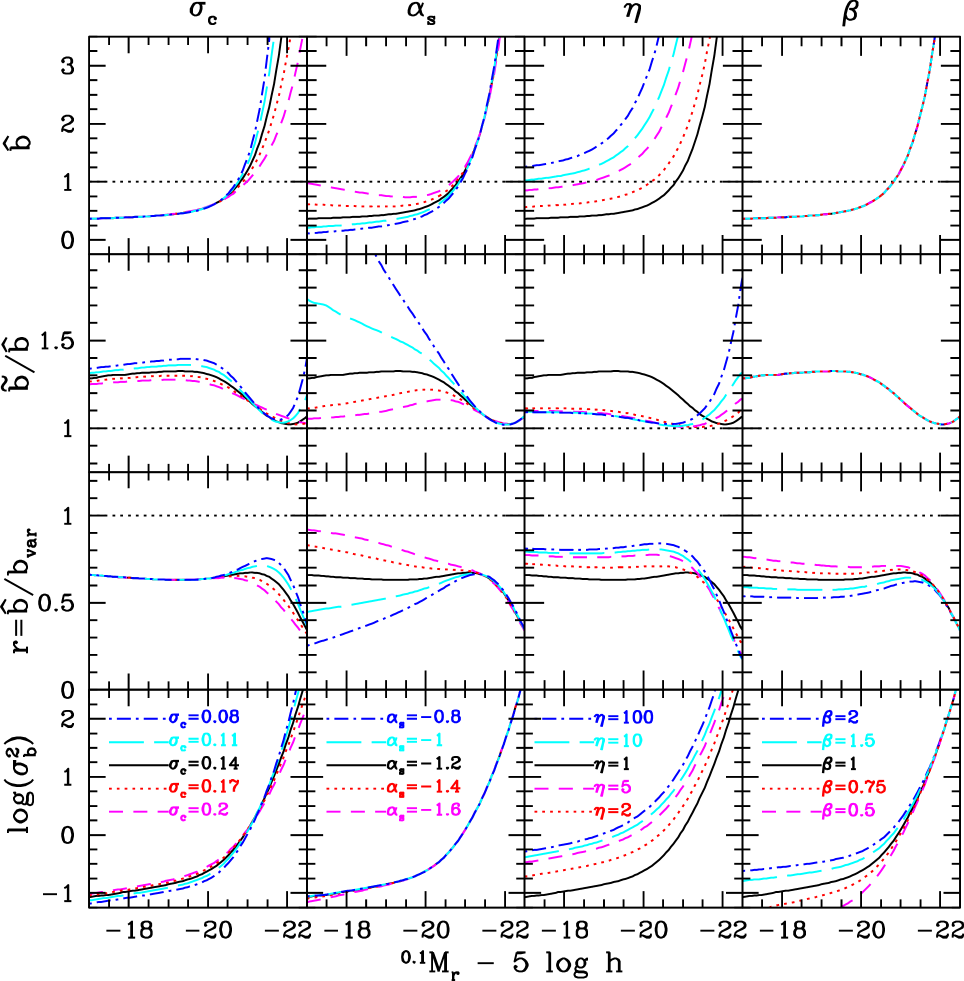
Figure 1: The dependence of galaxy bias on halo occupation statistics. From top to bottom, the various panels plot $\hat{b}$, the non-linearity parameter $\tilde{b}/\hat{b}$, the cross correlation coefficient $r$, and the stochasticity parameter $\log(\sigma_{\rm b}^{2})$ always for galaxies with luminosities in the range $[L_{1},2.5L_{1}]$. Results are plotted as function of $L_{1}$, expressed as an $r$-band magnitude that has been $K$+$E$ corrected to $z=0.1$. From left to right, we each time vary only one parameter (listed at the top) with respect to our fiducial model, which is indicated by the black, solid line. The horizontal, dotted line corresponds to linear, deterministic biasing. See eq.(29), (30),(33), and (25) for the definition of $\sigma_{\rm c},\alpha_{\rm s},\eta,$ and $\beta$, respectively.

Fig. 1 shows the parameters $\hat{b}$ (upper row), $\tilde{b}/\hat{b}$ (second row), $r$ (third row), and $\log(\sigma_{\rm b}^{2})$ (bottom row) as functions of $L_{1}$ (expressed in ${}^{0.1}M_{r}-5\log h$, which is the $r$-band magnitude $K$+$E$ corrected to $z=0.1$). Throughout we have adopted luminosity bins of one magnitude width, so that $L_{2}=2.5L_{1}$; hence, the value of $\hat{b}$ at ${}^{0.1}M_{r}-5\log h=-20$ indicates the first moment of the mean biasing function, $b(M)$, for galaxies with $-21\leq{{}^{0.1}M}_{r}-5\log h\leq-20$, etc. The solid curves in Fig. 1 show the results for our fiducial model ($\sigma_{\rm c}=0.14$; $\alpha_{\rm s}=-1.2$; $\eta=1.0$ and $\beta=1.0$), while the different columns show models in which we vary only one of the CLF parameters, as indicated. The parameter $\eta$ in the third column is defined by

$$\Phi(L|M)=\Phi_{\rm c}(L|M)/\eta+\Phi_{\rm s}(L|M)\,,$$ (33)

and is used to artificially reduce the contribution of centrals, simply by increasing $\eta$ with respect to its fiducial value. To guide the discussion, Fig. 2 shows the halo occupation distributions (HODs) corresponding to the various models shown in Fig. 1. Note how increasing $\sigma_{\rm c}$ broadens the contribution of centrals, how increasing $\alpha_{\rm c}$ reduces the slope ${\rm d}\log\langle N|M\rangle/{\rm d}\log M$, and how increasing $\eta$ suppresses the contribution of centrals.

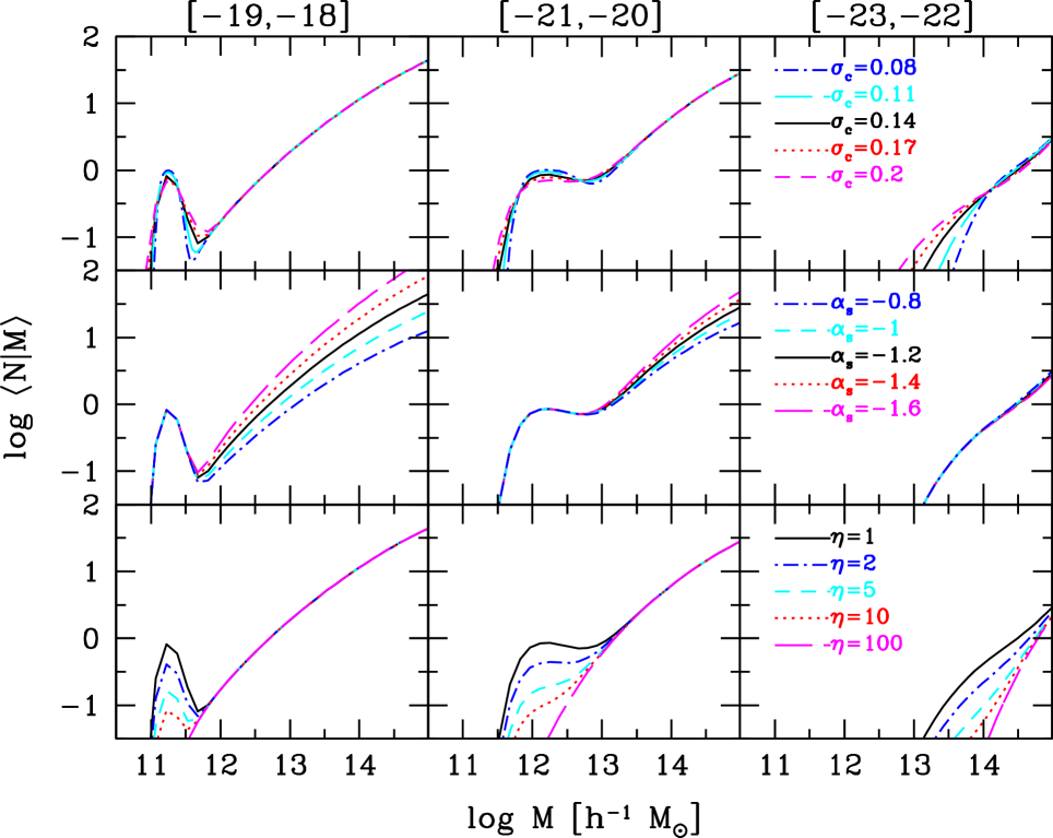
Figure 2: The halo occupation statistics, $\langle N|M\rangle$, as function of halo mass, $M$, for three different magnitude bins (different columns, as indicated at the top). From top to bottom we vary $\sigma_{\rm c}$, $\alpha_{\rm s}$ and $\eta$ with respect to our fiducial model, which is always indicated as a black, solid curve. These are the same HODs as used in Fig. 1. Note how increasing $\sigma_{\rm c}$ broadens the contribution of centrals, how increasing $\alpha_{\rm c}$ reduces the slope ${\rm d}\log\langle N|M\rangle/{\rm d}\log M$, and how increasing $\eta$ suppresses the contribution of centrals.

Starting with the upper panels of Figure 1, we see that the fiducial model predicts a $\hat{b}(L_{1})$ that strongly increases with luminosity. In order to understand this behavior, we use Eqs. (6) and (9) to write

$$\hat{b}={\bar{\rho}_{\rm m}\over\bar{n}_{\rm g}}\,{\int\langle N|M\rangle\,M\,n(M)\,{\rm d}M\over\int M^{2}\,n(M)\,{\rm d}M}$$ (34)

Hence, $\hat{b}=1$ if $\langle N|M\rangle=(\bar{n}_{\rm g}/\bar{\rho}_{\rm m})\,M$, which corresponds to $b(M)=1$. As evident from Fig. 2, for brighter bins, $\langle N|M\rangle$ cuts off at higher $M$ (i.e., bright galaxies can only reside in massive haloes), and this cut-off causes $\hat{b}>1$. For fainter galaxies, the contribution of central galaxies in the HOD becomes more pronounced, resulting in a ‘boost’ of $\langle N|M\rangle$ at relatively low $M$ (see left-hand panels of Fig. 2), which in turn results in $\hat{b}<1$. This is also evident from the scaling with $\eta$: increasing $\eta$ suppresses the relative contribution of centrals, which in turn causes an increase in $\hat{b}$. Changing the Poisson parameter only changes the scatter in the number of satellites, and therefore has no impact on $\hat{b}$ (or $\tilde{b}$), while changes in $\sigma_{\rm c}$ or $\alpha_{\rm s}$ has only a mild impact on $\hat{b}$ for reasons that are easily understood from an examination of Eq. (34) and Fig. 2. The main message here is that realistic HODs differ strongly from the simple scaling $\langle N|M\rangle\propto M$, such that $\hat{b}<1$ ($\hat{b}>1$) for faint (bright) galaxies.

The second row of panels in Fig. 1 shows that the ‘normalized’ non-linearity parameter $\tilde{b}/\hat{b}$ also differs markedly from unity for our fiducial model. As for $\hat{b}$, this parameter is also equal to unity if bias is linear (i.e., if $\langle N|M\rangle=(\bar{n}_{\rm g}/\bar{\rho}_{\rm m})\,M$). Since this is not the case for realistic HODs, both $\tilde{b}$ and $\hat{b}$ will in general differ from unity. At the faint-end, $\tilde{b}/\hat{b}$ is extremely sensitive to the parameter $\alpha_{\rm s}$. This is easy to understand; as is evident from Fig. 2, the parameter $\alpha_{\rm s}$ controls the slope of $\langle N|M\rangle$ at the massive end, especially for fainter galaxies, for which the satellite fraction is larger. Models for which the slope ${\rm d}\log\langle N|M\rangle/{\rm d}\log M$ deviates more from unity are more non-linear. In other words, $\tilde{b}/\hat{b}$ is simply a measure for how much $\langle N|M\rangle$ differs from the linear relation $\langle N|M\rangle\propto M$.

The third row of panels in Fig. 1 shows the cross-correlation coefficient $r$. In all cases shown, and for all luminosities, the CLF indicates that $r<1$. Writing that

$$r={\hat{b}\over\tilde{b}}\,\left[1+\left({\sigma_{\rm b}\over\tilde{b}}\right)^{2}\right]^{-1/2}\,,$$ (35)

we immediately see that $r\leq\hat{b}/\tilde{b}$ (where the equality corresponds to deterministic biasing). Hence, the fact that $r<1$ simply reflects the fact that, for realistic halo occupation statistics, the non-linearity parameter $\tilde{b}/\hat{b}>1$. The decline of $r$ at the bright-end is a reflection of stochasticity becoming more and more important for brighter galaxies. This is evident from the bottom panels of Fig. 1, which show that $\sigma_{\rm b}$ increases very strongly with luminosity. In order to understand this behavior, it is useful to rewrite Eq. (13) using Eqs. (26)-(27) as

$$\sigma_{\rm b}={1\over{\cal M}_{2}}\left[{1\over\bar{n}_{\rm g}}+{\cal I}(\beta)\right]^{1/2}\,,$$ (36)

where

$${\cal M}_{2}\equiv\left[\int\left({M\over\bar{\rho}_{\rm m}}\right)^{2}\,n(M)\,{\rm d}M\right]^{1/2}$$ (37)

is some constant, we have assumed that $N_{\rm c}$ and $N_{\rm s}$ are independent random variables, and

$${\cal I}(\beta) \equiv (\beta-1)\,f^{2}_{\rm s}\,\int{\langle N_{\rm s}|M\rangle^{2}\over\bar{n}_{\rm s}^{2}}\,n(M)\,{\rm d}M-$$ (38)

$$f^{2}_{\rm c}\,\int{\langle N_{\rm c}|M\rangle^{2}\over\bar{n}_{\rm c}^{2}}\,n(M)\,{\rm d}M\,.$$

Here $f_{\rm c}=\bar{n}_{\rm c}/\bar{n}_{\rm g}$ and $f_{\rm s}=\bar{n}_{\rm s}/\bar{n}_{\rm g}=1-f_{\rm c}$ are the central and satellite fractions, respectively, and the average number densities $\bar{n}_{\rm g}$, $\bar{n}_{\rm c}$ and $\bar{n}_{\rm s}$ follow from

$$\bar{n}_{\rm x}=\int\langle N_{\rm x}|M\rangle\,n(M)\,{\rm d}M\,,$$ (39)

where ‘x’ stands for ‘g’ (for galaxies), ‘c’ (for centrals) or ‘s’ (for satellites). The first term of Eq. (36) indicates the contribution to $\sigma_{\rm b}$ due to shot-noise, i.e., the finite number of galaxies (per halo). This term dominates when the number density of galaxies is small (i.e., for bright galaxies), in which case $\sigma_{\rm b}\propto\bar{n}_{\rm g}^{-1/2}$. It is this shot-noise that is responsible for driving $r\rightarrow 0$ at the bright end. The second term of Eq. (36) describes the contribution to $\sigma_{\rm b}$ due to specific aspects of the halo occupation statistics, as described by the function ${\cal I}(\beta)$. This function, which is independent of $\bar{n}_{\rm g}$, consists of two terms describing the contributions due to the possible non-Poissonian nature of satellite galaxies (i.e., if $\beta\neq 1$) and due to scatter in the occupation statistics of centrals (i.e., a non-zero $\sigma_{\rm c}$). Note that the first term of ${\cal I}$ is zero for our fiducial model, which has $\beta=1$. This explains the insensitivity to changes in $\alpha_{\rm s}$. Changes in $\sigma_{\rm c}$ only have a very mild impact on the stochasticity, while increasing (decreasing) $\beta$ only has a significant impact for faint galaxies, simply because the $1/\bar{n}_{\rm g}$ shot-noise term dominates for bright galaxies. Finally, the increase of $\sigma_{\rm b}$ with increasing $\eta$ is simply a reflection of the fact that an increase in $\eta$ reduces the number density of (central) galaxies.

To summarize, realistic halo occupation models predict a galaxy bias that is strongly non-linear, indicating that realistic models do not scale as $\langle N|M\rangle\propto M$. This is mainly a consequence of central galaxies, which dominate the number density and for which $\langle N_{\rm c}|M\rangle$ never resembles a power-law. However, even for satellite galaxies it is important to realize that $\langle N_{\rm s}|M\rangle$ never follows a pure power law; even if $\langle N_{\rm s}|M\rangle\propto M$ at the massive end, there will be a cut-off at low $M$, reflecting that galaxies of a given luminosity (or stellar mass) require a minimum mass for their host halo. Such a cut-off by itself is already sufficient to cause $\hat{b}$ and $\tilde{b}$ to deviate significantly from unity. As for the stochasticity; this is largely dominated by shot-noise, with halo-to-halo scatter, which reflects the second moment of the halo occupation distribution $P(N|M)$, only contributing significantly for fainter galaxies.

4 Two-Point Statistics

The bias parameters defined in §2 are quantities that are averaged over dark matter haloes. Given that (virtually) all galaxies are believed to reside in haloes, this is a logical and intuitive way to define galaxy bias. However, observationally it is far from trivial to actually measure these quantities from data. After all, this requires an observational method to identify individual dark matter haloes. In principle, this can be achieved using gravitational lensing, but in practice this is only possible for massive clusters. An alternative is to use a halo-based galaxy group finder, such as the one developed by Yang et al. (2005a). However, this method has the disadvantage that it uses galaxies to identify the dark matter haloes and estimate their masses. Consequently, $N$ and $M$ are not independent variables, which is likely to cause systematic errors. For example, if $N$ is in one way or the other used to estimate $M$, the halo-to-halo variance in $P(N|M)$, and hence the amount of stochasticity, will be underestimated.

Therefore, when the goal is to put constraints on galaxy bias using observational data, one requires another set of bias parameters that do not suffer from these shortcomings. Such a set can be defined using two-point statistics, such as the galaxy-galaxy and galaxy-matter correlation functions, which can be reliably measured from large galaxy surveys such as the SDSS. In addition, with the help of the ‘halo model’, which describes the dark matter density field in terms of its halo building blocks (see e.g., Cooray & Sheth 2002; Mo et al. 2010), one can analytically compute the galaxy-galaxy correlation function from the same occupation statistics, $P(N|M)$, required to compute $\hat{b}$, $\tilde{b}$, $b_{\rm var}$, $r$ and $\sigma_{\rm b}$.

Let us define the following two-point correlation functions:

$$\xi_{\rm gg}(r) \equiv \langle\delta_{\rm g}({\bf x})\delta_{\rm g}({\bf x}+{\bf r})\rangle$$

$$\xi_{\rm mm}(r) \equiv \langle\delta_{\rm m}({\bf x})\delta_{\rm m}({\bf x}+{\bf r})\rangle$$

$$\xi_{\rm gm}(r) \equiv \langle\delta_{\rm g}({\bf x})\delta_{\rm m}({\bf x}+{\bf r})\rangle\,,$$ (40)

where $\langle...\rangle$ represents an ensemble average, $r=|{\bf r}|$ is the distance between the two locations, and the subscripts ‘gg’, ‘gm’, ‘mm’ refer to ‘galaxy-galaxy’, ‘galaxy-matter’, and ‘matter-matter’, respectively.

Using these two-point correlation functions, we now define three functions that are sensitive to different aspects of galaxy bias: the ‘classical’ galaxy bias function,

$$b^{\rm 3D}_{\rm g}(r)\equiv\sqrt{\frac{\xi_{\rm gg}(r)}{\xi_{\rm mm}(r)}}\,,$$ (41)

the galaxy-dark matter cross-correlation coefficient (hereafter CCC),

$${\cal R}^{\rm 3D}_{\rm gm}(r)\equiv\frac{\xi_{\rm gm}(r)}{[\xi_{\rm gg}(r)*\xi_{\rm mm}(r)]^{1/2}}\,,$$ (42)

(Pen 1998), and their ratio,

$$\Gamma^{\rm 3D}_{\rm gm}(r)\equiv\frac{b^{\rm 3D}_{\rm g}(r)}{{\cal R}^{\rm 3D}_{\rm gm}(r)}=\frac{\xi_{\rm gg}(r)}{\xi_{\rm gm}(r)}\,.$$ (43)

The reason for introducing $\Gamma^{\rm 3D}_{\rm gm}$ is that, contrary to $b^{\rm 3D}_{\rm gm}$ and ${\cal R}^{\rm 3D}_{\rm gm}$ it is independent of the matter-matter correlation function, which makes it easier to measure observationally (see Sheldon et al. 2004). In what follows we shall loosely refer to these functions as ‘bias functions’, and to their $r$-dependence as ‘scale-dependence’.

Using the ergodic principle, the ensemble average, $\langle...\rangle$, can be written as a volume average, which in turn, under the assumption that all dark matter is bound in virialized dark matter haloes, is equal to an average over dark matter haloes (see Mo et al. 2010). Hence, similar to the bias parameters defined in §2, the bias functions $b^{\rm 3D}_{\rm g}(r)$, ${\cal R}^{\rm 3D}_{\rm gm}(r)$, and $\Gamma^{\rm 3D}_{\rm gm}(r)$ are also ‘defined’ as halo averaged quantities. The advantage of defining bias functions via two-point statistics, however, is that they can be measured without the need to identify individual dark matter haloes. Finally, we emphasize that the CCC is not restricted to $|{\cal R}(r)|\leq 1$ when computed with the analytical halo model because it intrinsically subtracts out the shot-noise term in the galaxy correlation (see e.g., Sheth & Lemson 1999; Seljak 2000).

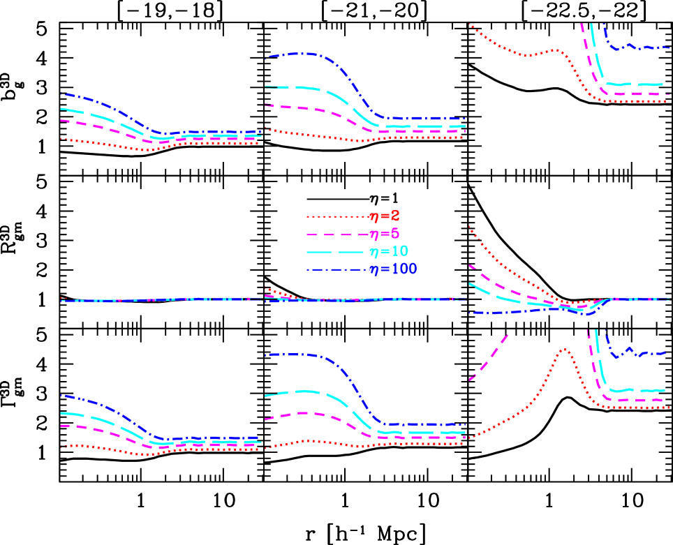
Figure 3: Scale dependence of the galaxy bias functions $b^{\rm 3D}_{\rm g}$, ${\cal R}^{\rm 3D}_{\rm gm}$, and $\Gamma^{\rm 3D}_{\rm gm}$ for three luminosity bins (indicated at the top of every column). The reference model is indicated with the black solid lines, whereas other lines refer to a suppression of the central term of the HOD by a factor $1/\eta$ (see eq. [33] and discussion in §3).

4.1 Analytical Model

As we shall see below, all these three bias functions can be computed analytically from the halo occupation distribution $P(N|M)$, making them the natural extension of the bias parameters defined in § 2 to the two-point regime. We address the observational perspective of these bias functions in §6. In this section we focus on investigating what realistic models for halo occupation statistics predict for (the scale dependence of) $b^{\rm 3D}_{\rm g}$, ${\cal R}^{\rm 3D}_{\rm gm}$ and $\Gamma^{\rm 3D}_{\rm gm}$.

In what follows we describe the two-point statistics in Fourier space, using power-spectra rather than two-point correlation functions. This has the single advantage that equations that involve convolutions in real-space can now be written in a more compact form. Throughout we assume that dark matter haloes are spherically symmetric and have a density profile, $\rho_{\rm m}(r|M)=M\,u_{\rm h}(r|M)$, that depends only on their mass, $M$. Note that $\int u_{\rm h}({\bf x}|M,z)\,{\rm d}^{3}{\bf x}=1$. Similarly, we assume that satellite galaxies in haloes of mass $M$ follow a spherical number density distribution $n_{\rm s}(r|M)=N_{\rm s}\,u_{\rm s}(r|M)$, while central galaxies always have $r=0$. Since centrals and satellites are distributed differently, we write the galaxy-galaxy power spectrum as

$$P_{\rm gg}(k)=f^{2}_{\rm c}P_{\rm cc}(k)+2f_{\rm c}f_{\rm s}P_{\rm cs}(k)+f^{2}_{\rm s}P_{\rm ss}(k)\,,$$ (44)

while the galaxy-dark matter cross power spectrum is given by

$$P_{\rm gm}(k)=f_{\rm c}P_{\rm cm}(k)+f_{\rm s}P_{\rm sm}(k)\,.$$ (45)

In addition, it is common practice to split two-point statistics into a 1-halo term (both points are located in the same halo) and a 2-halo term (the two points are located in different haloes). Following Cooray & Sheth 2002 and Mo et al. 2010, the 1-halo terms are

$$P^{\rm 1h}_{\rm cc}(k)={1\over\bar{n}_{\rm c}}\,,$$ (46)

$$P^{\rm 1h}_{\rm ss}(k)=\beta\int{\cal H}_{{\rm s}}^{2}(M)\,n(M)\,{\rm d}M\,,$$ (47)

and all other terms are given by

$$P^{\rm 1h}_{\rm xy}(k)=\int{\cal H}_{\rm x}(M)\,{\cal H}_{\rm y}(M)\,n(M)\,{\rm d}M\,.$$ (48)

Here ‘x’ and ‘y’ are either ‘c’ (for central), ‘s’ (for satellite), or ‘m’ (for matter), and we have defined

$${\cal H}_{\rm m}(M)={M\over\bar{\rho}_{\rm m}}\,\tilde{u}_{\rm h}(k|M)\,,$$ (49)

$${\cal H}_{\rm c}(M)={\langle N_{\rm c}|M\rangle\over\bar{n}_{{\rm c}}}\,,$$ (50)

and

$${\cal H}_{\rm s}(M)={\langle N_{\rm s}|M\rangle\over\bar{n}_{{\rm s}}}\,\tilde{u}_{\rm s}(k|M)\,,$$ (51)

with $\tilde{u}_{\rm h}(k|M)$ and $\tilde{u}_{\rm s}(k|M)$ the Fourier transforms of the halo density profile and the satellite number density profile, respectively, both normalized to unity. The various 2-halo terms are given by

$$P^{\rm 2h}_{{\rm x}{\rm y}}(k)=P_{\rm lin}(k)\,\int{\rm d}M_{1}\,{\cal H}_{\rm x}(M_{1})\,b_{\rm h}(M_{1})\,n(M_{1})$$ (52)

$$\int{\rm d}M_{2}\,{\cal H}_{\rm y}(M_{2})\,b_{\rm h}(M_{2})\,n(M_{2})\,,$$

where $P_{\rm lin}(k)$ is the linear power spectrum and $b_{\rm h}(M,z)$ is the halo bias function (e.g., Mo & White 1996). Note that in this formalism, the matter-matter power spectrum simply reads $P_{\rm mm}(k)=P^{\rm 1h}_{\rm mm}(k)+P^{\rm 2h}_{\rm mm}(k)\,.$

The two-point correlation functions corresponding to these power-spectra are obtained by simple Fourier transformation:

$$\xi_{\rm xy}(r)={1\over 2\pi^{2}}\int_{0}^{\infty}P_{\rm xy}(k)\,{\sin kr\over kr}\,k^{2}\,{\rm d}k\,,$$ (53)

Throughout this paper we adopt the halo mass functions and halo bias functions of Tinker et al. (2008) and Tinker et al. (2010), respectively.

We caution the reader that this particular implementation of the halo model is fairly simplified. In particular, it ignores two important effects: scale dependence of the halo bias function and halo-exclusion (i.e., the fact that the spatial distribution of dark matter haloes is mutually exclusive). As discussed in Tinker et al. (2005), both effects are important on intermediate scales (in the 1-halo to 2-halo transition region). Indeed, demonstrated in van den Bosch et al. (2012, in preparation), ignoring these effects can cause systematic errors in the two-point correlation functions on scales of $\sim 1-2h^{-1}\>{\rm Mpc}$ that are as large as 50 percent. However, detailed tests have shown that the bias functions (41)-(43), which are defined in terms of ratios of these correlation functions, are much more accurate (with typical errors $\lower 3.01385pt\hbox{$\;\buildrel<\over{\sim}\;$}10$ percent); i.e., to first order, by taking ratios, one is less sensitive to uncertainties in the halo model. This is why it is advantageous to use the bias functions, rather than the two-point correlation functions themselves, when trying to constrain particular aspects of galaxy bias. It is the purpose of this paper to explore how the (scale-dependence) of the bias functions depend on various properties related to halo occupation statistics.

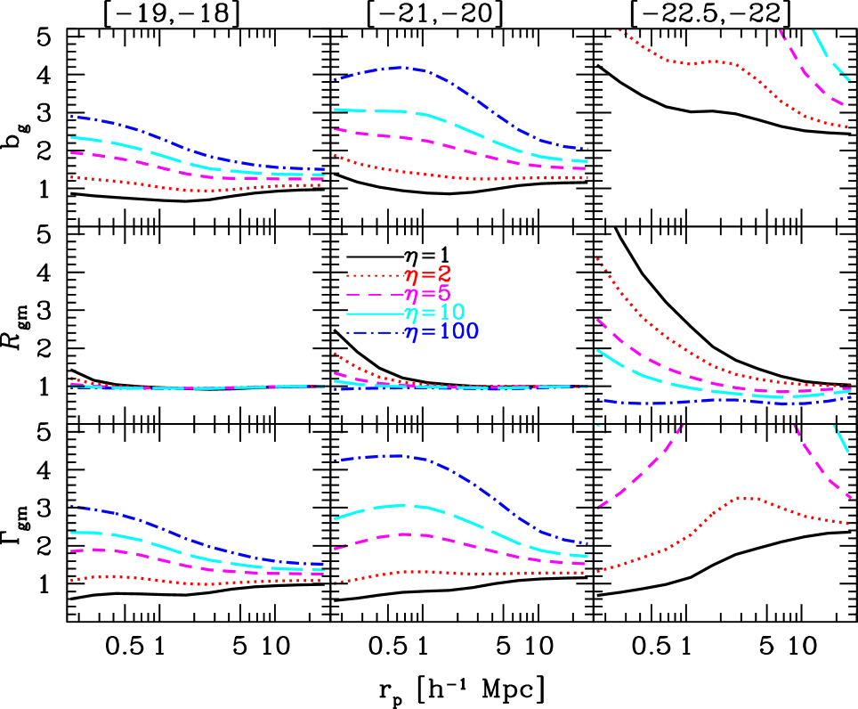
Figure 4: Scale dependence of the galaxy bias functions $b_{\rm g}$, ${\cal R}_{\rm gm}$, and $\Gamma_{\rm gm}$ for three luminosity bins (indicated at the top of every column). The reference model is indicated with the black solid lines, whereas other lines refer to a suppression of the central term of the HOD by a factor $1/\eta$ (see discussion in §3).

Before showing predictions based on a specific HOD, we can gain some insight from a closer examination of the above equations. In particular, it can easily be seen that galaxies are only unbiased with respect to the dark matter, at all scales (i.e., $b^{\rm 3D}_{\rm g}=1$), if and only if the following conditions are satisfied

1. $\eta=\infty$, i.e., there are no central galaxies

2. $\beta=1$, i.e., the occupation number of satellite galaxies obeys Poisson statistics

3. $u_{\rm s}(k|M)=u_{\rm h}(k|M)$, i.e., the normalized number density profile of satellite galaxies in dark matter haloes is identical to that of dark matter particles

4. $\langle N_{\rm s}|M\rangle={{\bar{n}}_{\rm s}\over\rho}M$, i.e., the occupation number of satellites is directly proportional to halo mass

Under these conditions one also has that ${\cal R}^{\rm 3D}_{\rm gm}=\Gamma^{\rm 3D}_{\rm gm}=1$. If all the above conditions are satisfied except that there is a non-negligble fraction of centrals (i.e., $\eta$ is finite), one expects strong scale-dependence on small scales due to the fact that the location of central galaxies within their dark matter haloes is strongly biased. If $\beta\neq 1$, one still maintains $b_{\rm g}^{\rm 3D}=1$ on large scales ($r\gg r_{12}$), but this will transit to $b_{\rm g}^{\rm 3D}=\beta$ for $r\ll r_{12}$ (if $\eta=\infty$). Here $r_{12}$ is the 1-halo to 2-halo transition region, which is roughly equal to the virial radius of the characteristic halo hosting the galaxies in question. This comes about because the Poisson parameter $\beta$ only enters in the 1-halo satellite-satellite term. If $\tilde{u}_{\rm s}(k|M)\neq\tilde{u}_{\rm h}(k|M)$, once again this will manifest itself as a transition from $b_{\rm g}^{\rm 3D}=1$ at $r\gg r_{12}$ to $b_{\rm g}^{\rm 3D}\neq 1$ at $r\ll r_{12}$ simply because $\tilde{u}_{\rm s}(k|M)=\tilde{u}_{\rm h}(k|M)=1$ on large scales (i.e., for $k\ll 1/r_{12}$). If $\langle N_{\rm s}|M\rangle$ is not proportional to $M$, which as we have seen in §3 is never expected to be the case for realistic HODs, one also expects a transition around $r_{12}$. However, in this case $b_{\rm g}^{\rm 3D}$ is not expected to be equal to unity at either small or large scales. The exact values of $b_{\rm g}^{\rm 3D}$ depend on how exactly the satellite occupation numbers deviate from linearity, but will be different on small and large scales mainly because the 2-halo term weights $\langle N_{\rm s}|M\rangle$ with the halo bias $b_{\rm h}(M)$, whereas the 1-halo term doesn’t. In fact, on large scales, where $\tilde{u}_{\rm s}(k|M)=\tilde{u}_{\rm h}(k|M)=1$ and the matter power spectrum is still in the linear regime, it is straightforward to show that

$$b^{\rm 3D}_{\rm g}={\langle M\,b(M)\,b_{\rm h}(M)\rangle\over\langle M\rangle}\,,$$ (54)

where $\langle...\rangle$ is the average over dark matter haloes given by Eq. (10) and $b(M)$ is the mean biasing function of Eq. (6). This immediately shows that the large scale bias $b_{\rm g}$ defined via the correlation functions cannot, in general, be expressed in terms of the moments $\hat{b}$ and $\tilde{b}$ of $b(M)$ (cf. Eq. [9]). Only in the case of linear biasing we have that $b^{\rm 3D}_{\rm g}=b(M)=\hat{b}=\tilde{b}=1$. To summarize, based on all these considerations, one expects scale independence on large scales, at a value that depends on the details of the HOD, a sudden transition at around the 1-halo to 2-halo transition scale, and scale dependence on small scales due to the dominance of central galaxies. Finally, it is worth pointing out that on the large scales where Eq. (54) is valid, one always expects that ${\cal R}^{\rm 3D}_{\rm gm}=1$ and $\Gamma^{\rm 3D}_{\rm gm}=b^{\rm 3D}_{\rm g}$.

Figure 3 shows the scale dependence of the biasing functions defined in Eqs. (41)-(43) computed using the analytic model outlined above and with the same halo occupation statistics as in §3. The three columns refer to three luminosity bins (expressed in r-band magnitude). Beside the reference model (black solid lines), we show four additional model predictions in which the contribution from central galaxies is increasingly suppressed as the parameter $\eta$ changes from unity to 100 (see discusssion in §3). As is evident from the upper panels, the galaxy bias, $b^{\rm 3D}_{\rm g}$, exactly reveals the behaviour expected based on the discussion above: on large scales the bias is scale-independent, there is sudden transition around the 1-halo to 2-halo transition scale (which is larger for brighter galaxies, since these reside in more massive, and therefore more extended haloes), and there is significant scale dependence on small scales. Note also that the large-scale bias is larger for brighter galaxies. This is consistent with observations (e.g., Guzzo et al. 2000; Norberg et al. 2001, 2002; Zehavi et al. 2005; Wang et al. 2007; Zehavi et al. 2011), and is a manifestation of the fact that brighter galaxies reside in more massive haloes, which are more strongly clustered (Mo & White 1996). The suppression of the contribution from central galaxies (i.e., increasing $\eta$) has the effect of increasing the value of the bias on large scales and it also affects the scale dependence of the bias on small scales. The effect is larger for brighter galaxies which is a direct consequence of the fact that, for realistic HODs the fraction of galaxies which are centrals is an increasing function of luminosity (e.g., Mandelbaum et al. 2006; van den Bosch et al. 2007; Cacciato et al. 2009).

As expected, the CCC, ${\cal R}_{\rm gm}^{\rm 3D}$, shown in the panels in the middle row, is unity on large scales for all three luminosity bins, and independent of the value of $\eta$. On small scales, however, ${\cal R}^{\rm 3D}_{\rm gm}>1$. This scale dependence is mainly due to the central galaxies being located at the centers of their dark matter haloes. Indeed, suppressing the contribution of central galaxies (i.e., increasing $\eta$) results in a CCC that is closer to unity on small scales. Overall, the scale dependence of ${\cal R}^{\rm 3D}_{\rm gm}$ is more pronounced for brighter galaxies. This is a consequence of the fact that brighter galaxies reside in more massive, and therefore more extended, haloes. Note that our model, which is based on a realistic HOD that is in excellent agreement with a wide range of data, predicts that for galaxies with magnitudes in the range $-18\geq^{0.1}M_{r}-5\log h\geq-19$ and $-20\geq^{0.1}M_{r}-5\log h\geq-21$ the CCC is very close to unity on scales above $r\lower 3.01385pt\hbox{$\;\buildrel>\over{\sim}\;$}0.2h^{-1}$ Mpc and $r\lower 3.01385pt\hbox{$\;\buildrel>\over{\sim}\;$}0.4h^{-1}$ Mpc, respectively. As we will see below, this is actually a very robust prediction, and indicates that if suppression of scale-dependence is important, it is in general advantageous to use fainter galaxies (but see §6.2). For the brightest bin, our model predicts that simply reducing the contribution from the central galaxies does not lead to ${\cal R}^{\rm 3D}_{\rm gm}=1$ over the scale probed here. This is due to the fact that a realistic HOD does not have $\langle N_{\rm s}|M\rangle\propto M$ and even more important bright satellite galaxies only form above a large halo mass. We have tested that artificially imposing $\langle N_{\rm s}|M\rangle\propto M$ and no low-mass cut off yields ${\cal R}^{\rm 3D}_{\rm gm}=1$ at all scales of interested here also in this brightest bin.

Finally, because of its definition, the scale dependence of the bias function $\Gamma^{\rm 3D}_{\rm gm}$, shown in the lower panels, is easily understood from a combination of the effects on both $b^{\rm 3D}_{\rm gm}$ and ${\cal R}^{\rm 3D}_{\rm gm}$. Our fiducial model predicts that $\Gamma^{\rm 3D}_{\rm gm}$ is scale-independent on large scales, and decreases with decreasing radius on small scales where the 1-halo term of the two-point correlation functions dominates. Overall, the scale-dependence of $\Gamma^{\rm 3D}_{\rm gm}$ is predicted to be larger for brighter galaxies.

The results in Fig. 3 indicate that our analytical model, which is based on a realistic HOD, makes some very specific predictions regarding the scale dependence of the bias functions (41)-(43). However, before we embark on a detailed study of how these predictions depend on some specific aspects of the halo occupation model used, it is important to stress that the results in Fig. 3 are in real-space. Unfortunately, because of redshift-space distortions and projection effects, real-space correlation functions are extremely difficult, if not impossible, to obtain observationally. We therefore first recast our bias functions into two-dimensional, projected analogues, which are more easily accessible observationally. We start by defining the matter-matter, galaxy-matter, and galaxy-galaxy projected surface densities as

$$\Sigma_{\rm xy}(r_{\rm p})=2{\bar{\rho}}\,\int_{r_{\rm p}}^{\infty}\left[1+\xi_{\rm xy}(r)\right]\,{r{\rm d}r\over\sqrt{r^{2}-r_{\rm p}^{2}}}\,,$$ (55)

where ‘x’ and ‘y’ stand either for ‘g’ or ‘m’, and $r_{\rm p}$ is the projected separation. We also define $\overline{\Sigma}_{\rm xy}(<r_{\rm p})$ as its average inside $r_{\rm p}$, i.e.

$$\bar{\Sigma}_{\rm xy}(<r_{\rm p})=\frac{2}{r^{2}_{\rm p}}\int_{0}^{r_{\rm p}}\Sigma_{\rm xy}(R^{\prime})R^{\prime}dR^{\prime}\,,$$ (56)

which we use to define the excess surface densities

$$\Delta\Sigma_{\rm xy}(r_{\rm p})=\bar{\Sigma}_{\rm xy}(<r_{\rm p})-\Sigma_{\rm xy}(r_{\rm p})\,.$$ (57)

These can subsequently be used to define the projected, 2D analogues of Eqs. (41)-(43) as

$$b_{\rm g}(r_{\rm p})\equiv\sqrt{\frac{\Delta\Sigma_{\rm gg}(r_{\rm p})}{\Delta\Sigma_{\rm mm}(r_{\rm p})}}\,,$$ (58)

$${\cal R}_{\rm gm}(r_{\rm p})\equiv\frac{\Delta\Sigma_{\rm gm}(r_{\rm p})}{\sqrt{\Delta\Sigma_{\rm gg}(r_{\rm p})\,\Delta\Sigma_{\rm mm}(r_{\rm p})}}\,,$$ (59)

and

$$\Gamma_{\rm gm}(r_{\rm p})\equiv\frac{b_{\rm g}(r_{\rm p})}{{\cal R}_{\rm gm}(r_{\rm p})}=\frac{\Delta\Sigma_{\rm gg}(r_{\rm p})}{\Delta\Sigma_{\rm gm}(r_{\rm p})}\,,$$ (60)

In what follows we shall refer to these as the ‘projected bias functions’.

Note that in the case of the galaxy-dark matter cross correlation, the excess surface density $\Delta\Sigma_{\rm gm}(r_{\rm p})=\gamma_{\rm t}(r_{\rm p})\,\Sigma_{\rm crit}$, where $\gamma_{\rm t}(r_{\rm p})$ is the tangential shear which can be measured observationally using galaxy-galaxy lensing, and $\Sigma_{\rm crit}$ is a geometrical parameter that depends on the comoving distances of the sources and lenses. In the case of the galaxy-galaxy autocorrelation we can write that

$$\Delta\Sigma_{\rm gg}(r_{\rm p})=\bar{\rho}\left[{2\over r^{2}_{\rm p}}\int_{0}^{r_{\rm p}}w_{\rm p}(R^{\prime})\,R^{\prime}\,{\rm d}R^{\prime}-w_{\rm p}(r_{\rm p})\right]\,,$$ (61)

from which it is immediately clear that $\Delta_{\rm gg}(r_{\rm p})$ is straightforwardly obtained from the projected correlation function $w_{\rm p}(r_{\rm p})$, which is routinely measured in large galaxy redshift surveys. Finally, in the case of the matter-matter autocorrelation, the quantity $\Delta\Sigma_{\rm mm}(r_{\rm p})$ can be obtained observationally if accurate cosmic shear measurements are available. Since the cosmic shear measurements are the most challenging, the parameter $\Gamma_{\rm gm}(r_{\rm p})$, which is independent of $\Delta\Sigma_{\rm mm}(r_{\rm p})$, is significantly easier to determine observationally than either $b_{\rm g}(r_{\rm p})$ and/or ${\cal R}_{\rm gm}(r_{\rm p})$. In fact, current clustering and galaxy-galaxy lensing data from the SDSS is already of sufficient quality to allow for reliable measurements of $\Gamma_{\rm gm}(r_{\rm p})$ for different luminosity bins. The purpose of this paper, however, is not to perform such measurements, but rather to provide theoretical guidance on how to constrain different aspects of galaxy biasing by exploiting the wealth of information encoded in the scale dependence of the (projected) galaxy bias functions.

5 Impact of halo occupation assumptions on galaxy biasing

We now investigate how modifications of the halo occupation statistics, modelled via the CLF, impact the projected bias functions $b_{\rm g}(r)$, ${\cal R}_{\rm gm}(r)$ and $\Gamma_{\rm gm}(r)$ defined in Eqs. (58)-(60). We first study modifications regarding the way central galaxies occupy dark matter haloes, followed by an indepth study of the impact of various aspects of satellite occupation statistics.

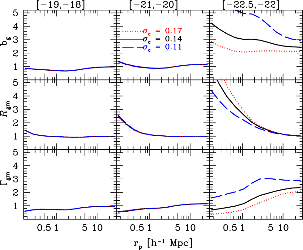
Figure 5: Same as in Fig. 4. The reference model is indicated with the black solid lines, whereas other lines refer to models with larger ($\sigma_{\rm c}=0.17$, red dotted lines) or smaller ($\sigma_{\rm c}=0.11$, blue dashed lines) scatter in the luminosity-halo mass relation (see eq. [29] and discussion in §5.2).

5.1 The Relative Contribution of Centrals

We start by exploring the role of central galaxies by comparing models in which the relative contribution of centrals is progressively suppressed via the parameter $\eta$ (see §3). Figure 4 shows the scale dependence of the projected bias functions $b_{\rm g},{\cal R}_{\rm gm},\Gamma_{\rm gm}$ for the same luminosity bins as in Figure 3. The bias functions are plotted as a function of the projected radius, $r_{\rm p}$, covering the range [0.1, 30]$h^{-1}$ Mpc. Results are shown for the reference model ($\eta=1$, black solid lines) and for models with an increasingly lower contribution from centrals ($\eta=2,5,10,100$, as indicated). Overall, the trends are very similar to those seen in Fig. 3. For instance, the reference model once again shows that the magnitude of scale dependence increases with luminosity. However, upon closer examination some important differences become apparent, which arise from projecting and integrating the two-point correlation functions, which are the operations performed in order to compute the excess surface densities given by Eq. [57]. An important difference is that the galaxy bias, $b_{\rm g}$, remains scale dependent out to much larger radii; in the highest luminosity bin, significant scale dependence remains visible out to $\sim 20h^{-1}\>{\rm Mpc}$. This is very different from the case of $b_{\rm g}^{\rm 3D}$ which becomes scale-independent at $\sim 5h^{-1}\>{\rm Mpc}$, independent of the value of $\eta$. This difference is a consequence of the integration (56), which mixes in signal from small scales. This mixing also smears out the sharp features in the 1-halo to 2-halo transition region that are present in their 3D analogues. Hence, although the projected bias functions have the advantage that they are observationally accessible, their interpretation is less straightforward. Nevertheless, as we will see below, different aspects of the halo occupation statistics impact the projected bias functions in sufficiently different ways that they still provide valuable insight into the nature of galaxy biasing.

5.2 Scatter in the Luminosity-Halo Mass Relation

Throughout this paper, the number of central galaxies with luminosity $L$ that reside in a halo of mass $M$ is modelled as a log-normal distribution (see Eq. [29]), whose standard deviation, $\sigma_{\rm c}$, indicates the scatter in luminosity at a given halo mass. Following Cacciato et al. (2009), and motivated by the results of More et al. (2009b) based on satellite kinematics, we assume that $\sigma_{\rm c}$ is independent of halo mass. Cacciato et al. (2009) obtained $\sigma_{\rm c}=0.14$, which is the value we adopt in our fiducial reference model.

Figure 5 shows the projected galaxy bias functions for the reference model ($\sigma_{\rm c}=0.14$, black solid lines) and for two models with $\sigma_{\rm c}=0.17$ (red dotted lines) and $\sigma_{\rm c}=0.11$ (blue dashed lines), respectively. All other parameters are kept unchanged. Only the brightest bin reveals appreciable changes in the bias functions. This is most easily understood by examining the upper panels of Fig. 2, which show how changes in $\sigma_{\rm c}$ impact the occupation statistics. For the two fainter bins, changes in $\sigma_{\rm c}$ only have a very mild impact on the HODs. This in turn is a consequence of the fact that fainter galaxies reside, on average, in less massive haloes, and therefore probe the low mass end of the halo mass function. In this regime, the halo mass function is a power law and variations in the scatter in $\Phi_{\rm c}(L|M)$ have little effect on the resulting mass of the average halo hosting these galaxies. Conversely, brighter galaxies probe the high mass end of the halo mass function, which reveals an exponential decline. Thus, variations in the scatter in $\Phi_{\rm c}(L|M)$ strongly affect the resulting mass of the average halo hosting these galaxies (see upper right-hand panel of Fig. 2), which reflects itself in a change of $b_{\rm g}$. In particular, increasing (decreasing) $\sigma_{\rm c}$ strongly suppresses (boosts) the bias $b_{\rm g}(r)$.

An interesting aspect of scatter (i.e., stochasticity) in the occupation statistics of central galaxies, is that it impacts the 2-halo term, i.e., changes in $\sigma_{\rm c}$ have an impact on $b_{\rm g}$ and $\Gamma_{\rm gm}$, but not ${\cal R}_{\rm gm}$, on large scales. This is a consequence of the fact that changes in $\sigma_{\rm c}$ impact $\langle N_{\rm c}|M\rangle$ (see discussion in §2.3). Note that this is not the case for the stochasticity of satellite galaxies, which only impacts the bias functions on small scales (where the 1-halo term dominates).

5.3 The First Moment of $P(N_{\rm s}|M)$

The first moment, $\langle N_{\rm s}|M\rangle$, of $P(N_{\rm s}|M)$, for any luminosity bin $[L_{1},L_{2}]$, is completely specified by the CLF (see § 3). As shown in Fig. 2, the slope of $\langle N_{\rm s}|M\rangle$ is very sensitive to changes in the parameter $\alpha_{\rm s}$, which controls the faint-end slope of $\Phi_{\rm s}(L|M)$: in general, smaller (i.e., more negative) values of $\alpha_{\rm s}$ result in steeper $\langle N_{\rm s}|M\rangle$. As such, $\alpha_{\rm s}$ is a parameter that controls the non-linearity of the HOD. Data from clusters and galaxy groups typically indicate values for $\alpha_{\rm s}$ in the range $-1.5\lower 3.01385pt\hbox{$\;\buildrel<\over{\sim}\;$}\alpha_{\rm s}\lower 3.01385pt\hbox{$\;\buildrel<\over{\sim}\;$}-0.9$ (e.g., Beijersbergen et al. 2002; Trentham & Tully 2002; Eke et al. 2004; Yang et al. 2008)

Figure 6 shows the projected bias functions for the reference model (which has $\alpha_{\rm s}=-1.2$) as well as for two variations with $\alpha_{\rm s}=-0.8$ and $-1.6$, as indicated. All other model parameters are kept unchanged. Note how smaller values of $\alpha_{\rm s}$ increase (decrease) the bias parameter $b_{\rm g}$ for faint (bright) galaxies. For faint galaxies, this is easy to understand; a more negative $\alpha_{\rm s}$ results in a steeper $\langle N_{\rm s}|M\rangle$, which implies that satellites, on average, reside in more massive (i.e., more strongly biased) haloes. Since the satellite fraction decreases with increasing luminosity, the impact of changes in $\alpha_{\rm s}$ become smaller for brighter galaxies.

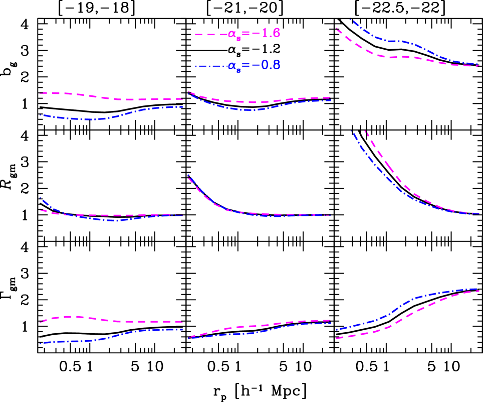
Figure 6: Same as in Fig. 4. The reference model is indicated with the black solid lines, whereas other lines refer to models with lower ($\alpha_{\rm s}=-1.6$, magenta dashed lines) or higher ($\alpha_{\rm s}=-0.8$, blue dot-dashed lines) value of the low mass end power-law index of the CLF (see eq.[30] and discussion in §5.3).

5.4 The Second Moment of $P(N_{\rm s}|M)$

The CLF does not specify the second moment, $\langle N_{\rm s}^{2}|M\rangle$, of the satellite occupation distribution. Rather, it is often assumed that $P(N_{\rm s}|M)$ follows a Poisson distribution

$$P(N_{\rm s}|M)=\frac{\lambda^{N_{\rm s}}\exp{[-\lambda]}}{N_{\rm s}!}\,,$$ (62)

where $\lambda=\langle N_{\rm s}|M\rangle$ is the first moment of the distribution. Recall that for a Poisson distribution all moments can be derived from the first moment. In particular, $\langle N_{\rm s}(N_{\rm s}-1)|M\rangle=\langle N_{\rm s}|M\rangle^{2}$. The assumption that $P(N_{\rm s}|M)$ is (close to) Poissonian has strong support from galaxy group catalogs (e.g., Yang et al. 2008) and from numerical simulations, which show that dark matter subhaloes (which are believed to host satellite galaxies) also follow Poisson statistics (Kravtsov et al. 2004). However, a number of studies have shown that there may be small but significant deviations from pure Poisson statisitcs (e.g., Porciani et al. 2004; van den Bosch et al. 2005a; Giocoli et al. 2010; Boylan-Kolchin et al. 2010; Busha et al. 2011). Hence, we investigate how deviations from Poisson, as parameterized via the parameter $\beta$ (see eq. 25), impact on the (projected) bias functions.

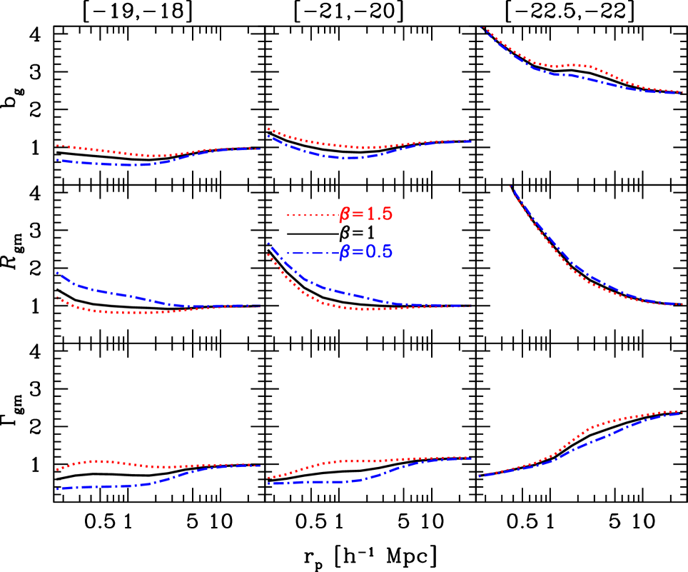
Figure 7: Same as in Fig. 4. The reference model is indicated with the black solid lines, whereas other lines refer to models with larger ($\beta=1.5$, red lines) or smaller ($\beta=0.5$, blue lines) Poisson parameter (see eq.[25] and discussion in §5.4).

Figure 7 shows the projected bias functions for the reference model ($\beta=1$, corresponding to $P(N_{\rm s}|M)$ being Poissonian) as well as for two variations with $\beta=0.5$ and $1.5$, as indicated. All other model parameters are kept unchanged. The parameter $\beta$ only affects the 1-halo satellite-satellite term of the galaxy-galaxy correlation function. This term typically has a maximum contribution close to the 1-halo to 2-halo transition region, which is therefore the radial interval that is most sensitive to changes in $\beta$. Since brighter galaxies reside in more massive (and therefore more extended) haloes, changes in $\beta$ impact the (projected) bias functions on larger scales for brighter galaxies. Also, since the satellite fraction increases with decreasing luminosity, the impact of changes in $\beta$ is larger for less luminous galaxies. Overall, though, changes in $\beta$ of 50 percent only have a fairly modest impact on the (projected) bias functions. Since $\beta$ is unlikely to differ from unity by more than $\sim 20$ percent, we conclude that potential deviations from Poisson statistics are unlikely to have a significant effect on galaxy biasing.

5.5 The Spatial Distribution of Satellites

In our fiducial reference model it is assumed that the number density distribution of satellites within dark matter haloes is identical to that of dark matter particles; i.e., we assume that $\tilde{u}_{\rm s}(k|M)=\tilde{u}_{\rm h}(k|M)$. The dark matter density profiles are modelled as NFW (Navarro et al. 1997) profiles, with a concentration mass relation, $c_{\rm h}(M)$, given by Macciò et al. (2007). Whether the assumption that the number density distribution of satellite galaxies is well described by the same NFW profile, and with the same concentration-mass relation, is still unclear. In particular, numerous studies have come up with conflicting claims (e.g., Beers & Tonry 1986; Carlberg et al. 1997; van der Marel et al. 2000; Lin et al. 2004; van den Bosch et al. 2005b; Yang et al. 2005b; Chen 2009; More et al. 2009a; Nierenberg et al. 2011; Watson et al. 2011; Guo et al. 2012). We therefore examine the impact of changing the number density profiles of satellites, which we parameterize via

$$f_{\rm conc}=c_{\rm s}/c_{\rm h}\,,$$ (63)

where $c_{\rm s}$ is the concentration parameter of the satellite number density profile. Note that $f_{\rm conc}=1$ for our fiducial reference model. Figure 8 shows how changes in $f_{\rm conc}$ impact the projected bias functions. The various curves correspond to $f_{\rm conc}=0.5$, $1.0$ and $2.0$, as indicated. All other model parameters are the same as for the reference model. As expected, changing the radial number density profile of satellite galaxies only affects the bias functions on small scales where the 1-halo term dominates. In general, a more centrally concentrated distribution of satellites (i.e., larger $f_{\rm conc}$) results in a larger galaxy bias and smaller CCC on small scales. Since the impact of $f_{\rm conc}$ is restricted to smaller scales than most other changes in the halo occupation statistics, accurate measurements of the (projected) bias functions on small scales holds excellent potential for constraining the radial number density profiles of satellite galaxies.

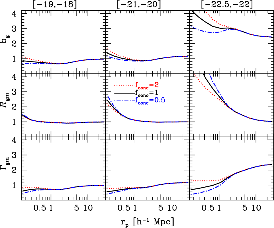
Figure 8: Same as in Fig. 4. The reference model is indicated with the black solid lines, whereas other lines refer to models with higher ($f_{\rm conc}=2$, red dotted lines) or lower ($f_{\rm conc}=0.5$, blue dot-dashed lines) value of the ratio between dark matter and galaxy concentration, $f_{\rm conc}=c_{\rm m}/c_{\rm g}$. (see eq. [63] and discussion in §5.5).

6 Observational Perspective

6.1 Probing the Scale Dependence of Galaxy Bias

Constraining the non-linearity and stochasticity of galaxy bias with observations is a non-trivial task. The main reason is that it requires measurements of the fluctuations in the matter density (or $n$-point statistics thereof), which are difficult to obtain. In the absence of such information, however, one can still make some progress. For example, one can test for linearity by measuring higher-order statistics of the galaxy distribution, such as the bi-spectrum (e.g., Frieman & Gaztañaga 1999; Szapudi et al. 2002; Verde et al. 2002). This method, though, yields no information regarding stochasticity in the relation between galaxies and matter. Alternatively, Tegmark & Bromley (1999) suggested a method to constrain the non-linearity and/or stochasticity by comparing different samples of galaxies (i.e., different luminosity bins, early-types vs. late-types, etc.) Quoting directly from their paper: “If two different types of galaxies are both perfectly correlated with the matter, they must also be perfectly correlated with each other”. Hence, if one can establish that the correlation between the two samples is imperfect, than galaxy bias has to be non-linear and/or stochastic for at least one of the two samples. Different implementations of this idea have been used by a number of authors (e.g., Blanton 2000; Conway et al. 2005; Wild et al. 2005; Wang et al. 2007; Swanson et al. 2008; Zehavi et al. 2011), with the general result that bias cannot be linear and deterministic.

A third method to constrain the non-linearity of galaxy bias without direct measurements of the matter fluctuations was proposed by Sigad et al. (2000). Here the idea is to measure the probability distribution function (PDF) ${\cal P}(\delta_{\rm g})$ of the galaxy field using counts-in-cells measurements, and to compare that with (log-normal) models for the PDF ${\cal P}(\delta_{\rm m})$ of mass fluctuations. Under the assumption that the bias relation between galaxies and matter is deterministic and monotonic, one can use these two PDFs to infer the conditional mean bias relation $\langle\delta_{\rm g}|\delta_{\rm m}\rangle$. This method has been applied to the first epoch VIMOS VLT deep survey (VVDS; Le Fèvre et al. 2005) by Marinoni et al. (2005) and to the zCOSMOS survey (Lilly et al. 2007) by Kovač et al. (2011). Both studies find clear indications that bias is non-linear. However, this method has a number of important shortcomings: it assumes that bias is deterministic, is cosmology-dependent, and, because it has to filter the galaxy distribution (typically on scales of $5-10h^{-1}\>{\rm Mpc}$) is carries no information of galaxy bias on small scales. As we have shown, these are the scales that carry most information regarding the non-linearity and stochasticity of galaxy bias.

Arguably the most promosing method to measure non-linearity and stochasticity in galaxy bias, which does not require any assumptions regarding cosmology or bias, is to use a combination of galaxy clustering and gravitational lensing. The latter is the only direct probe of the matter distribution in the Universe, and allows for direct measurements of the galaxy-matter cross correlation (via galaxy-galaxy lensing) as well as the matter auto-correlation (via cosmic shear). When combined with the galaxy-galaxy correlation, these measurements yield the bias functions $b_{\rm g}(r)$, ${\cal R}_{\rm gm}(r)$ and $\Gamma_{\rm gm}(r)$ discussed in this paper. As elucidated above, the scale dependence of these bias functions holds great promise to gain valuable insight into the origin of non-linearity and stochasticity of galaxy bias.

Pen et al. (2003) applied these ideas to the VIRMOS-DESCART cosmic shear survey (Van Waerbeke et al. 2000). Using deprojection techniques, they computed the 3D power spectra for dark matter and galaxies, as well as their cross correlation. They find a weak indication of scale dependence with ${\cal R}^{\rm 3D}_{\rm gm}$ decreasing with scale, in qualitative agreement with the predictions shown in §5. van Waerbeke (1998) and Schneider (1998) proposed a somewhat alternative application of this method based on aperture masses and aperture number counts. The aperture mass, $M_{\rm ap}(\theta)$, is defined as

$$M_{\rm ap}(\theta)=\int{\rm d}^{2}\phi\,U(\phi)\,\delta^{\rm 2D}_{\rm m}(\phi)\,,$$ (64)

(Schneider et al. 1998), where $\delta^{\rm 2D}_{\rm m}$ is the projected mass overdensity and $U(\phi)$ is a compensated filter, i.e. $\int{\rm d}\phi\,\phi\,U(\phi)=0$ and $U(\phi)=0$ for $\phi>\theta$. Similarly, for galaxies one defines the aperture number count

$$N_{\rm ap}(\theta)=\int{\rm d}^{2}\phi\,U(\phi)\,\delta^{\rm 2D}_{\rm g}(\phi)\,,$$ (65)

with $\delta^{\rm 2D}_{\rm g}$ the projected galaxy overdensity. The mass autocorrelation function $\langle M^{2}_{\rm ap}(\theta)\rangle$ can be derived from the observed ellipticity correlation functions, the angular two-point correlation function of galaxies yields $\langle N^{2}_{\rm ap}(\theta)\rangle$, and the ensemble-averaged tangential shear as a function of radius around a sample of lenses (galaxy-galaxy lensing signal) can be used to derive $\langle N_{\rm ap}(\theta)M_{\rm ap}(\theta)\rangle$ (Van Waerbeke et al. 2002; Hoekstra et al. 2002). Relating these variances at a given smoothing aperture, $\theta$, one obtains the aperture bias functions

$$b_{\rm ap}(\theta)\propto\frac{\langle N^{2}_{\rm ap}(\theta)\rangle}{\langle M^{2}_{\rm ap}(\theta)\rangle}\,,$$ (66)

and

$${\cal R}_{\rm ap}(\theta)\propto\frac{\langle N_{\rm ap}(\theta)M_{\rm ap}(\theta)\rangle}{\sqrt{\langle N^{2}_{\rm ap}(\theta)\rangle\langle M^{2}_{\rm ap}(\theta)\rangle}}\,,$$ (67)

where the constants of proportionality depend in principle on the distribution of galaxies and on the assumed cosmological model (van Waerbeke 1998), although minimally within the current uncertainties on cosmological parameters (Komatsu et al. 2011).

The aperture-based method has been applied to data from the RCS (Yee & Gladders, 2002) in Hoekstra et al. (2001) and in combination with data from the VIRMOS-DESCART survey in Hoekstra et al. (2002). Their results indicate that $b_{\rm ap}$ and ${\cal R}_{\rm ap}$ are scale-dependent over scales $\sim 0.1-5h^{-1}\>{\rm Mpc}$, but that the ratio $\Gamma_{\rm ap}\equiv b_{\rm ap}/{\cal R}_{\rm ap}$ is nearly constant at $\Gamma_{\rm ap}\sim 1.1$ over this range. On scales of $\sim 0.5h^{-1}\>{\rm Mpc}$, they find that $b_{\rm ap}=0.71^{+0.06}_{-0.05}$ and ${\cal R}_{\rm ap}\sim 0.59^{+0.08}_{-0.07}$ (68% confidence, assuming a flat $\Lambda$CDM cosmology with $\Omega_{\rm m}=0.3$). In Fig. 9, we show a revised version of the analysis published in Hoekstra et al. (2002), which was based on the cosmic shear analysis of Van Waerbeke et al. (2002). However, as discussed in Van Waerbeke et al. (2005), these data suffered from PSF anisotropy that was not corrected for. Figure 9 shows the new results obtained using the same cosmology as in Hoekstra et al. (2002), the unchanged RCS measurements and the Van Waerbeke et al. (2005) cosmic shear results. Compared to the results in Hoekstra et al. (2002), the scale dependence on small scales has been somewhat reduced. On scales of $\sim 0.5h^{-1}\>{\rm Mpc}$, the new analysis suggests $b_{\rm ap}=0.96^{+0.09}_{-0.07}$ and ${\cal R}_{\rm ap}=0.74^{+0.12}_{-0.09}$ (68% confidence).

The finding that $b_{\rm ap}(\theta)$ and ${\cal R}_{\rm ap}(\theta)$ have similar scale dependence so that $\Gamma_{\rm ap}(\theta)$ is nearly scale independent (over the scales probed) seems at odds with the predictions in §5. However, we caution that the bias parameters based on aperture variances are different from the ones investigated in this paper, which are based on excess surface densities. Furthermore, lacking any redshift information, Hoekstra et al. (2002) used a (apparent) magnitude selected sample which mixes galaxies of different intrinsic luminosity and different physical scales. Hence, one cannot directly compare our model predictions (Figs. 4-8) with the data in Fig. 9. On the other hand, the difference between aperture variances and excess surface densities is mainly operational, rather than conceptual, and it is difficult to imagine that they would predict very different scale dependencies. In that respect it is interesting that a more recent study by Jullo et al. (2012), using the same aperture variance analysis, but applied to data from the COSMOS survey (Scoville et al. 2007), obtain $b_{\rm ap}(\theta)$ and ${\cal R}_{\rm ap}(\theta)$ that more closely follow the trends shown in Figs. 4-8. We intend to interpret these aperture variance data within the context of halo occupation statistics in a future publication.

Figure 9: The scale dependence of the galaxy bias (top panel) and the cross-correlation coefficient (bottom panel) as measured with the aperture mass rechnique in the RCS survey (see discussion in §6.1), properly accounting for PSF anisotropy (following Van Waerbeke et al. 2005).

Finally, we emphasize that the galaxy-matter cross correlation is a first-order measure of the cosmic shear and therefore much easier to measure than the matter auto-correlation, which is second-order (see e.g., Schneider 1998). Hence, the bias parameter $\Gamma_{\rm gm}$ can typically be measured with significantly smaller error bars than either $b_{\rm g}$ or ${\cal R}_{\rm gm}$, simply because it does not require the matter-matter correlation function. As we have shown in this paper, the scale dependene of $\Gamma_{\rm gm}$, even the one defined via the projected surface densities, contains a wealth of information regarding the non-linearity and stochasticity of the halo occupation statistics, and thus regarding galaxy formation. Sheldon et al. (2004) used galaxy clustering and galaxy-galaxy lensing data from the SDSS in order to measure $\Gamma^{\rm 3D}_{\rm gm}(r)$ for a large sample of $\sim 100,000$ galaxies. Using Abel integrals, they deproject their data in order to estimate the 3D galaxy-galaxy and galaxy-matter correlation functions. The resulting $\Gamma^{\rm 3D}_{\rm gm}(r)$ is found to be roughly scale-invariant over the radial range $0.2h^{-1}\>{\rm Mpc}\lower 3.01385pt\hbox{$\;\buildrel<\over{\sim}\;$}r\lower 3.01385pt\hbox{$\;\buildrel<\over{\sim}\;$}6.7h^{-1}\>{\rm Mpc}$ at a value of $(1.3\pm 0.2)\,(\Omega_{\rm m}/0.27)$. Note that the galaxies used in this measurement cover a wide range in magnitudes, making it difficult to compare directly to the ‘predictions’ in Figs. 4-8. It would be interesting to repeat these measurements using narrower luminosity bins extracted from the significantly larger and more accurate SDSS data samples currently available. We advocate to perform such an analysis using the projected surface densities (Eq. [57]), rather than the deprojected 3D quantities used by Sheldon et al. (2004).

6.2 Suppressing the Scale Dependence of Galaxy Bias

For some applications, it is desirable to have bias functions with as little scale-dependence as possible. As discussed in §5.1, because of the integration performed when calculating the observable, projected bias functions, signal on small scales is mixed-in on large scales. This causes the scale above which the bias functions are scale-independent to increase. A constraint on the amount of scale-dependence therefore means that a large fraction of the data would have to be discarded. This can be mitigated, however, by defining alternative bias functions that circumvent mixing-in signal form small scales. For instance, Reyes et al. (2010) used the quantities

$$\Upsilon_{\rm xy}(r_{\rm p})\equiv\Delta\Sigma_{\rm xy}(r_{\rm p})-\left({r_{\rm min}\over r_{\rm p}}\right)^{2}\Delta\Sigma_{\rm xy}(r_{\rm min})$$ (68)

which are directly related to the excess surface densities defined in Eq. (57), and where $r_{\rm min}$ is some fiducial length scale. By rewriting Eq. (68) as

$$\Upsilon_{\rm xy}(r_{\rm p}) = {2\over r^{2}_{\rm p}}\int_{r_{\rm min}}^{r_{\rm p}}\Sigma_{\rm xy}(R^{\prime})\,R^{\prime}\,{\rm d}R^{\prime}\,-\Sigma_{\rm xy}(r_{\rm p})$$ (69)

$$+ \left({r_{\rm min}\over r_{\rm p}}\right)^{2}\Sigma_{\rm xy}(r_{\rm min})$$

it is immediately clear that $\Upsilon_{\rm xy}$ does not include any contribution from length scales smaller than $r_{\rm min}$. Hence, one could opt to define the projected bias functions (58)-(60) using $\Upsilon_{\rm xy}(r_{\rm p})$ rather than $\Delta\Sigma_{\rm xy}(r_{\rm p})$. In what follows we shall indicate these new bias functions as $\widehat{b}_{\rm g}$, $\widehat{{\cal R}}_{\rm gm}$ and $\widehat{\Gamma}_{\rm gm}$, respectively.

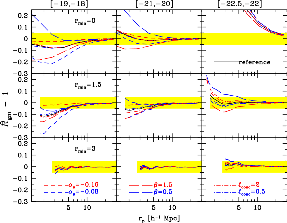
Figure 10: The quantity $\widehat{{\cal R}}_{\rm gm}(r_{\rm p})-1$ for three different values of $r_{\rm min}$ (different rows), and for three magnitude bins (different columns). The black solid curve corresponds to our fiducial reference model, while other curves correspond to several variations discussed in §5 (as indicated in the bottom panels). The shaded area indicates the region where scale dependence of $\widehat{{\cal R}}_{\rm gm}(r_{\rm p})$ yields values close to unity within 5%.

Reyes et al. (2010) used galaxy clustering, galaxy-galaxy lensing and peculiar velocities of luminous red galaxies (LRGs) from the SDSS to measure the probe of gravity (Zhang et al. 2007)

$$E_{\rm G}(r_{\rm p})\equiv{1\over\widehat{\beta}}{\Upsilon_{\rm gm}(r_{\rm p})\over\Upsilon_{\rm gg}(r_{\rm p})}=f(\Omega_{\rm m})\,\widehat{{\cal R}}_{\rm gm}(r_{\rm p})\,,$$ (70)

where $\widehat{\beta}=f(\Omega_{\rm m})/b_{\rm g}$ is the redshift distortion parameter (not to be confused with the Poisson parameter $\beta$), which can be measured from the redshift space correlation function (e.g., Tegmark et al. 2006), $f(\Omega_{\rm m})\approx\Omega_{\rm m}^{0.55}$ is the logarithmic linear growth rate, and $b_{\rm g}$ is the galaxy bias. As long as $\widehat{{\cal R}}_{\rm gm}(r_{\rm p})=1$, which can be assured by picking a sufficiently large $r_{\rm min}$, it is clear that $E_{\rm G}$ is a direct probe of $f(\Omega_{\rm m})$, which is sensitive to modifications of the law of gravity. In their analysis, Reyes et al. (2010) adopt $r_{\rm min}=1.5h^{-1}\>{\rm Mpc}$.

We now use our models to investigate the amount of scale dependence in $\widehat{{\cal R}}_{\rm gm}(r_{\rm p})$ for various values of $r_{\rm min}$. Fig. 10 plots $\widehat{{\cal R}}_{\rm gm}(r_{\rm p})-1$ for three different values of $r_{\rm min}$ (different rows), and for three magnitude bins (different columns). The solid curve corresponds to our fiducial reference model, while other curves correspond to several variations with respect to this model discussed in §5 (as indicated in the bottom panels). The shaded area indicates the region where scale dependence of $\widehat{{\cal R}}_{\rm gm}(r_{\rm p})$ affects the measurement of $E_{\rm G}$ at less than five percent.

In the upper panels we set $r_{\rm min}=0$, for which $\widehat{{\cal R}}_{\rm gm}(r_{\rm p})$ reduces to ${\cal R}_{\rm gm}(r_{\rm p})$. As we have already seen, this CCC reveals very strong scale-dependence, especially for bright galaxies, making ${\cal R}_{\rm gm}(r_{\rm p})$ useless for measuring $E_{\rm G}$. For $r_{\rm min}=1.5h^{-1}\>{\rm Mpc}$ (panels in middle row), this scale dependence is drastically reduced, in particular for the brightest galaxies. Note, though, that depending on the exact values of $\alpha_{\rm s}$, $f_{\rm conc}$ and $\beta$ the CCC $\widehat{{\cal R}}_{\rm gm}(r_{\rm p})$ may still differ from unity at the 10 to 20 percent level on small scales ($r_{\rm p}\sim r_{\rm min}$). However, adopting $r_{\rm min}=3h^{-1}\>{\rm Mpc}$ (lower panels) yields $\widehat{\Gamma}_{\rm gm}(r_{\rm p})=1$ to better than 5 percent accuracy for all luminosity bins, and with very little dependence on uncertainties regarding the halo occupation statistics. Hence, we conclude that the method used by Reyes et al. (2010) succesfully suppresses the scale-dependence of galaxy bias. For $r_{\rm min}=1.5h^{-1}\>{\rm Mpc}$, which is the value adopted by Reyes et al. (2010) in their analysis of LRGs in the SDSS, our models suggest, though, that there may be some residual scale dependence on small scales at the 10-20 percent level, depending on detailed aspects of the halo occupation statisitics. We find that robustly suppressing scale dependence in $\widehat{{\cal R}}_{\rm gm}(r_{\rm p})$ to better than five percent requires $r_{\rm min}\lower 3.01385pt\hbox{$\;\buildrel>\over{\sim}\;$}3h^{-1}\>{\rm Mpc}$.

Finally, we emphasize that the bias functions $\widehat{b}_{\rm g}(r_{\rm p})$, $\widehat{{\cal R}}_{\rm gm}(r_{\rm p})$ and $\widehat{\Gamma}_{\rm gm}(r_{\rm p})$ should only be used if one is interested in suppressing scale-dependence. If, on the other hand, one is interested in using two-point statistics to unveil the nature of galaxy bias, which is the main goal of this paper, one should use the projected bias functions (58)-(60) instead.

7 Summary and Conclusions

Studying galaxy bias is important for furthering our understanding of galaxy formation, and for being able to use the distribution of galaxies to constrain cosmology. Despite a large number of (both observational and theoretical) studies, we still lack a useful framework for translating constraints on galaxy biasing as inferred from observations into constraints on the theory of galaxy formation.

In an attempt to improve this situation, we have reformulated the parameterization of non-linear and stochastic biasing introduced by Dekel & Lahav (1999; DL99) in the framework of halo occupation statistics. The bias parameters introduced by DL99 relate the smoothed density field, $\delta_{\rm g}$, to the smoothed matter field, $\delta_{\rm m}$. This smoothing, however, has a number of shortcomings. First, there is considerable loss of information on small scales (below the filtering scale), which, as we have shown in this paper, carry most information regarding galaxy bias. Second, the smoothing procedure is extremely sensitivity to (arbitrary) filtering scale: if the filtering scale is too large, the data has too little dynamic range to probe the non-linearity in the galaxy bias. A filtering scale that is too small, on the other hand, results in too much shot-noise. Finally, the smoothing technique hampers an intuitive link to the theory of galaxy formation.

Since galaxies are believed to form and reside in dark matter haloes, it is far more natural, and intuitive, to define halo averaged quantities (i.e., to adopt the host halo as the ‘filtering’ scale). This automatically suggest a reformulation of the DL99 parameterization in terms of halo occupation statistics. Since dark matter haloes are biased entities themselves, such a formulation has the additional advantage that the overall bias of galaxies has a natural ‘split’ in two components: (i) how haloes are biased with respect to the dark matter mass distribution, and (ii) how galaxies are biased with respect to the haloes in which they reside. The former has been addressed in detail with $N$-body simulations (e.g., Mo & White 1996; Catelan et al. 1998; Porciani et al. 1999; Sheth & Lemson 1999). The latter has been the focus of this paper.

We have reformulated DL99 by replacing the filtered matter overdensity, $\delta_{\rm m}$, with halo mass, $M$, and the filtered galaxy overdensity, $\delta_{\rm g}$, with the occupation number, $N$. Within this modified framework, the sources of non-linearity and stochasticty in galaxy bias have logical and intuitive connections to various aspect of galaxy formation. In particular, non-linearity refers to deviations from $\langle N|M\rangle\propto M$, while stochasticity refers to scatter in the probability distribution function $P(N|M)$. Based on our basic understanding of galaxy formation, it is essentially impossible to have linear galaxy biasing. First of all, since galaxies of a given luminosity (or stellar mass) are only expected to form in haloes above some minimum mass, one always expects that $\langle N|M\rangle$ has some cut-off at low $M$. Furthermore, there is no convincing reason why $\langle N|M\rangle$ should scale linearly with halo mass above this mass scale. In particular, since $\langle N|M\rangle=\langle N_{\rm c}|M\rangle+\langle N_{\rm c}|M\rangle$, and $0\leq\langle N_{\rm c}|M\rangle\leq 1$, the contribution due to centrals typically gives rise to strong non-linearity. As for stochasticity, centrals contribute from the fact that there is non-zero scatter in the relation between halo mass and the luminosity of central galaxies (e.g., More et al. 2009b). The contribution from satellites comes from scatter in the halo occupation distribution $P(N_{\rm s}|M)$. Finally, an additional source of stochasticity may come about if $N_{\rm c}$ and $N_{\rm s}$ are not independent random variables.

A powerful method to probe the non-linearity and stochasticity of galaxy bias is via two-point correlation functions. In particular, non-linearity and stochasticty manifest themselves as scale dependence in the bias parameter $b^{\rm 3D}_{\rm g}(r)\equiv\xi_{\rm gg}(r)/\xi_{\rm mm}(r)$, and the galaxy-matter cross correlation parameter ${\cal R}^{\rm 3D}_{\rm gm}(r)\equiv\xi_{\rm gm}(r)/\sqrt{\xi_{\rm gg}(r)\,\xi_{\rm mm}(r)}$. In this paper we have proposed a modified set of bias parameters, $b_{\rm g}(r_{\rm p})$ and ${\cal R}_{\rm gm}(r_{\rm p})$, that are related to excess surface densities, rather than real-space correlation functions. These have the advantage that they can be inferred from data in a straightforward manner, without the need for complicated, and noise-enhancing, deprojection methods. In particular, combining galaxy clustering and galaxy-galaxy lensing, it is straightforward to measure the ratio $\Gamma_{\rm gm}(r_{\rm p})\equiv b_{\rm g}(r_{\rm p})/{\cal R}_{\rm gm}(r_{\rm p})$.

Using the halo model and a realistic halo occupation model, based on the conditional luminosity function of Cacciato et al. (2009), we have investigated how deviations from the linear and deterministic biasing scheme manifest themselves in the scale dependence of $b_{\rm g}$, ${\cal R}_{\rm gm}$, and $\Gamma_{\rm gm}$. In particular, we have compared predictions covering the spatial scale $0.1\leq r_{\rm p}\leq 30$ Mpc and for galaxies in three $r$-band magnitude bins; [-19,-18], [-21,-20], and [-22.5,-22]. These choices aim at bracketing the range of interest for current and forthcoming galaxy surveys.

We have shown that galaxy biasing is scale independent, with ${\cal R}^{\rm 3D}_{\rm gm}=1$, on large scales down to about $r\sim 2-5h^{-1}\>{\rm Mpc}$. The exact radius at which ${\cal R}^{\rm 3D}_{\rm gm}$ (and $b^{\rm 3D}_{\rm g}$) become scale dependent depends on luminosity, with fainter galaxies remaining scale independent down to smaller scales. This result is robust to all the model variations we have performed, but it is only valid in real-space. When using the projected bias parameters advocated here, which are more easily accessible observationally, the associated quantity ${\cal R}_{\rm gm}$ remains scale dependent out to much larger radii (as far out as $\sim 20h^{-1}\>{\rm Mpc}$). This comes about because the excess surface densities at projected radius $r_{\rm p}$ contain information from all scales $r\leq r_{\rm p}$. This ‘scale-mixing’ can be avoided by using the relative excess surface densities (see Baldauf et al. 2010; Reyes et al. 2010), which do not include any contribution from length scales smaller than some fiducial radius $r_{\rm min}$. Indeed, our models indicate that bias parameters based on these relative excess surface densities are scale independent at better than 5 percent for $r_{\rm min}\geq 3h^{-1}\>{\rm Mpc}$. For $r_{\rm min}=1.5h^{-1}\>{\rm Mpc}$, which is the value used by Reyes et al. (2010) in their study to test the validity of GR, we find residual scale dependence on small scales $r_{\rm p}\sim r_{\rm min}$ of the order of 20 percent.

On small scales ($r_{\rm p}\lower 3.01385pt\hbox{$\;\buildrel<\over{\sim}\;$}2-5h^{-1}\>{\rm Mpc}$), the bias functions $b_{\rm g}(r_{\rm p})$ and ${\cal R}_{\rm gm}(r_{\rm p})$ reveal strong scale dependence. The detailed behavior of $b_{\rm g}(r_{\rm p})$ and ${\cal R}_{\rm gm}(r_{\rm p})$ depends on (i) the luminosity of the galaxies in question, with more luminous galaxies typically revealing stronger scale-dependence, (ii) the detailed behavior of the occupation statistics, $\langle N|M\rangle$, (iii) the scatter in the relation between halo mass and the luminosity of central galaxies, $\sigma_{\rm c}$, (iv) whether the satellite occupation distribution $P(N_{\rm s}|M)$ is Poissonian or not, and (v) the radial number density distribution of galaxies within their host halo. For bright galaxies (${}^{0.1}M_{r}-5\log h\lower 3.01385pt\hbox{$\;\buildrel<\over{\sim}\;$}-20$), the dominant effect giving rise to the scale-dependence of ${\cal R}_{\rm gm}(r_{\rm p})$ is the precence of central galaxies, which occupy very biased regions of their host haloes. For fainter galaxies, ${\cal R}_{\rm gm}(r_{\rm p})$ is expected to be close to unity, down to $r_{\rm p}\sim 0.2h^{-1}\>{\rm Mpc}$, but with some dependence on the Poisson parameter $\beta$. Finally, we stress that $b_{\rm g}(r_{\rm p})$ and ${\cal R}_{\rm gm}(r_{\rm p})$ for the brightest galaxies are extremely sensitive to the amount of scatter, $\sigma_{\rm c}$, in the relation between halo mass and the luminosity of central galaxies.

We conclude that, since different aspects of halo occupation statistics impact the bias functions $b_{\rm g}(r_{\rm p})$ and ${\cal R}_{\rm gm}(r_{\rm p})$ in different ways, there is great promise to unveil the nature of galaxy bias from measurements of $b_{\rm g}(r_{\rm p})$ and ${\cal R}_{\rm gm}(r_{\rm p})$, (or from related quantities, such as the aperture-based bias parameters introduced by Schneider (1998) and van Waerbeke (1998)). Motivated by existing and forthcoming imaging and spectroscopic galaxy surveys, we advocate using a combination of clustering and galaxy-galaxy lensing to determine the ratio of $\Gamma_{\rm gm}=b_{\rm g}/{\cal R}_{\rm gm}$, as a function of the spatial scale $r_{\rm p}$ for a number of different luminosity (and/or stellar mass) bins. Inspired by the preliminary work of Sheldon et al. 2004, we intend to perform such an analysis in the near future, using data from the SDSS.

References

- Adelman-McCarthy et al. (2006) Adelman-McCarthy J. K. et al., 2006, ApJS, 162, 38
- Babul & White (1991) Babul A., White S. D. M., 1991, MNRAS, 253, 31P
- Baldauf et al. (2010) Baldauf T., Smith R. E., Seljak U., Mandelbaum R., 2010, PhysRevD, 81, 063531
- Bardeen et al. (1986) Bardeen J. M., Bond J. R., Kaiser N., Szalay A. S., 1986, ApJ, 304, 15
- Beers & Tonry (1986) Beers T. C., Tonry J. L., 1986, ApJ, 300, 557
- Beijersbergen et al. (2002) Beijersbergen M., Hoekstra H., van Dokkum P. G., van der Hulst T., 2002, MNRAS, 329, 385
- Berlind & Weinberg (2002) Berlind A. A., Weinberg D. H., 2002, ApJ, 575, 587
- Blanton (2000) Blanton M., 2000, ApJ, 544, 63
- Boylan-Kolchin et al. (2010) Boylan-Kolchin M., Springel V., White S. D. M., Jenkins A., 2010, MNRAS, 406, 896
- Braun et al. (1988) Braun E., Dekel A., Shapiro P. R., 1988, ApJ, 328, 34
- Busha et al. (2011) Busha M. T., Wechsler R. H., Behroozi P. S., Gerke B. F., Klypin A. A., Primack J. R., 2011, ApJ, 743, 117
- Cacciato et al. (2009) Cacciato M., van den Bosch F. C., More S., Li R., Mo H. J., Yang X., 2009, MNRAS, 394, 929
- Carlberg et al. (1997) Carlberg R. G., Yee H. K. C., Ellingson E., 1997, ApJ, 478, 462
- Catelan et al. (1998) Catelan P., Lucchin F., Matarrese S., Porciani C., 1998, MNRAS, 297, 692
- Cen & Ostriker (1992) Cen R., Ostriker J. P., 1992, ApJL, 399, L113
- Chen (2009) Chen J., 2009, A&A, 494, 867
- Collister & Lahav (2005) Collister A. A., Lahav O., 2005, MNRAS, 361, 415
- Conway et al. (2005) Conway E. et al., 2005, MNRAS, 356, 456
- Cooray & Milosavljević (2005) Cooray A., Milosavljević M., 2005, ApJL, 627, L89
- Cooray & Sheth (2002) Cooray A., Sheth R., 2002, Phys. Rep., 372, 1
- Davis et al. (1985) Davis M., Efstathiou G., Frenk C. S., White S. D. M., 1985, ApJ, 292, 371
- Dekel & Lahav (1999) Dekel A., Lahav O., 1999, ApJ, 520, 24
- Dekel & Rees (1987) Dekel A., Rees M. J., 1987, Nature, 326, 455
- Dekel & Silk (1986) Dekel A., Silk J., 1986, ApJ, 303, 39
- Eke et al. (2004) Eke V. R. et al., 2004, MNRAS, 355, 769
- Frieman & Gaztañaga (1999) Frieman J. A., Gaztañaga E., 1999, ApJ, 521, L83
- Gaztañaga et al. (2011) Gaztañaga E., Eriksen M., Crocce M., Castander F., Fosalba P., Marti P., Miquel R., Cabre A., 2011, ArXiv e-prints
- Giocoli et al. (2010) Giocoli C., Tormen G., Sheth R. K., van den Bosch F. C., 2010, MNRAS, 404, 502
- Guo et al. (2012) Guo Q., Cole S., Eke V., Frenk C., 2012, ArXiv e-prints
- Guzzo et al. (2000) Guzzo L. et al., 2000, A&A, 355, 1
- Hoekstra et al. (2002) Hoekstra H., van Waerbeke L., Gladders M. D., Mellier Y., Yee H. K. C., 2002, ApJ, 577, 604
- Hoekstra et al. (2001) Hoekstra H., Yee H. K. C., Gladders M. D., 2001, apjl, 558, L11
- Jing et al. (1998) Jing Y. P., Mo H. J., Boerner G., 1998, ApJ, 494, 1
- Jullo et al. (2012) Jullo E. et al., 2012, ArXiv e-prints
- Kaiser (1984) Kaiser N., 1984, apjl, 284, L9
- Kauffmann et al. (1997) Kauffmann G., Nusser A., Steinmetz M., 1997, MNRAS, 286, 795
- Komatsu et al. (2011) Komatsu E. et al., 2011, ApJS, 192, 18
- Kovač et al. (2011) Kovač K. et al., 2011, ApJ, 731, 102
- Kravtsov et al. (2004) Kravtsov A. V., Berlind A. A., Wechsler R. H., Klypin A. A., Gottlöber S., Allgood B., Primack J. R., 2004, ApJ, 609, 35
- Lahav & Saslaw (1992) Lahav O., Saslaw W. C., 1992, ApJ, 396, 430
- Laureijs et al. (2011) Laureijs R. et al., 2011, ArXiv e-prints
- Le Fèvre et al. (2005) Le Fèvre O. et al., 2005, A&A, 439, 845
- Lilly et al. (2007) Lilly S. J. et al., 2007, ApJS, 172, 70
- Lin et al. (2004) Lin Y.-T., Mohr J. J., Stanford S. A., 2004, ApJ, 610, 745
- Ma & Fry (2000) Ma C.-P., Fry J. N., 2000, ApJ, 543, 503
- Macciò et al. (2007) Macciò A. V., Dutton A. A., van den Bosch F. C., Moore B., Potter D., Stadel J., 2007, MNRAS, 378, 55
- Mandelbaum et al. (2006) Mandelbaum R., Seljak U., Kauffmann G., Hirata C. M., Brinkmann J., 2006, MNRAS, 368, 715
- Marinoni et al. (2005) Marinoni C. et al., 2005, A&A, 442, 801
- Mo et al. (2010) Mo H., van den Bosch F. C., White S., 2010, Galaxy Formation and Evolution. Cambridge University Press
- Mo & White (1996) Mo H. J., White S. D. M., 1996, MNRAS, 282, 347
- More et al. (2009a) More S., van den Bosch F. C., Cacciato M., 2009a, MNRAS, 392, 917
- More et al. (2009b) More S., van den Bosch F. C., Cacciato M., Mo H. J., Yang X., Li R., 2009b, MNRAS, 392, 801
- Navarro et al. (1997) Navarro J. F., Frenk C. S., White S. D. M., 1997, ApJ, 490, 493
- Nierenberg et al. (2011) Nierenberg A. M., Auger M. W., Treu T., Marshall P. J., Fassnacht C. D., 2011, ApJ, 731, 44
- Norberg et al. (2002) Norberg P. et al., 2002, MNRAS, 332, 827
- Norberg et al. (2001) Norberg P. et al., 2001, MNRAS, 328, 64
- Peacock & Smith (2000) Peacock J. A., Smith R. E., 2000, MNRAS, 318, 1144
- Pen (1998) Pen U.-L., 1998, ApJ, 504, 601
- Pen et al. (2003) Pen U.-L., Lu T., van Waerbeke L., Mellier Y., 2003, MNRAS, 346, 994
- Porciani et al. (1999) Porciani C., Catelan P., Lacey C., 1999, apjl, 513, L99
- Porciani et al. (2004) Porciani C., Magliocchetti M., Norberg P., 2004, MNRAS, 355, 1010
- Reyes et al. (2010) Reyes R., Mandelbaum R., Seljak U., Baldauf T., Gunn J. E., Lombriser L., Smith R. E., 2010, Nature, 464, 256
- Scherrer & Weinberg (1998) Scherrer R. J., Weinberg D. H., 1998, ApJ, 504, 607
- Schneider (1998) Schneider P., 1998, ApJ, 498, 43
- Schneider et al. (1998) Schneider P., van Waerbeke L., Jain B., Kruse G., 1998, MNRAS, 296, 873
- Scoville et al. (2007) Scoville N. et al., 2007, ApJS, 172, 1
- Seljak (2000) Seljak U., 2000, MNRAS, 318, 203
- Sheldon et al. (2004) Sheldon E. S. et al., 2004, AJ, 127, 2544
- Sheth & Lemson (1999) Sheth R. K., Lemson G., 1999, MNRAS, 304, 767
- Sigad et al. (2000) Sigad Y., Branchini E., Dekel A., 2000, ApJ, 540, 62
- Simon et al. (2007) Simon P., Hetterscheidt M., Schirmer M., Erben T., Schneider P., Wolf C., Meisenheimer K., 2007, A&A, 461, 861
- Somerville et al. (2001) Somerville R. S., Lemson G., Sigad Y., Dekel A., Kauffmann G., White S. D. M., 2001, MNRAS, 320, 289
- Spergel et al. (2007) Spergel D. N. et al., 2007, ApJS, 170, 377
- Swanson et al. (2008) Swanson M. E. C., Tegmark M., Blanton M., Zehavi I., 2008, MNRAS, 385, 1635
- Szapudi et al. (2002) Szapudi I. et al., 2002, ApJ, 570, 75
- Taruya & Soda (1999) Taruya A., Soda J., 1999, ApJ, 522, 46
- Tegmark & Bromley (1999) Tegmark M., Bromley B. C., 1999, apjl, 518, L69
- Tegmark et al. (2006) Tegmark M. et al., 2006, PhysRevD, 74, 123507
- Tegmark & Peebles (1998) Tegmark M., Peebles P. J. E., 1998, apjl, 500, L79+
- Tinker et al. (2008) Tinker J., Kravtsov A. V., Klypin A., Abazajian K., Warren M., Yepes G., Gottlöber S., Holz D. E., 2008, ApJ, 688, 709
- Tinker et al. (2010) Tinker J. L., Robertson B. E., Kravtsov A. V., Klypin A., Warren M. S., Yepes G., Gottlöber S., 2010, ApJ, 724, 878
- Tinker et al. (2005) Tinker J. L., Weinberg D. H., Zheng Z., Zehavi I., 2005, ApJ, 631, 41
- Trentham & Tully (2002) Trentham N., Tully R. B., 2002, MNRAS, 335, 712
- van den Bosch et al. (2005a) van den Bosch F. C., Tormen G., Giocoli C., 2005a, MNRAS, 359, 1029
- van den Bosch et al. (2005b) van den Bosch F. C., Yang X., Mo H. J., Norberg P., 2005b, MNRAS, 356, 1233
- van den Bosch et al. (2007) van den Bosch F. C. et al., 2007, MNRAS, 376, 841
- van der Marel et al. (2000) van der Marel R. P., Magorrian J., Carlberg R. G., Yee H. K. C., Ellingson E., 2000, AJ, 119, 2038
- van Waerbeke (1998) van Waerbeke L., 1998, A&A, 334, 1
- Van Waerbeke et al. (2000) Van Waerbeke L. et al., 2000, A&A, 358, 30
- Van Waerbeke et al. (2005) Van Waerbeke L., Mellier Y., Hoekstra H., 2005, A&A, 429, 75
- Van Waerbeke et al. (2002) Van Waerbeke L., Mellier Y., Pelló R., Pen U.-L., McCracken H. J., Jain B., 2002, A&A, 393, 369
- Verde et al. (2002) Verde L. et al., 2002, MNRAS, 335, 432
- Wang et al. (2007) Wang Y., Yang X., Mo H. J., van den Bosch F. C., 2007, ApJ, 664, 608
- Watson et al. (2011) Watson D. F., Berlind A. A., McBride C. K., Hogg D. W., Jiang T., 2011, ArXiv e-prints
- Wild et al. (2005) Wild V. et al., 2005, MNRAS, 356, 247
- Yang et al. (2003) Yang X., Mo H. J., van den Bosch F. C., 2003, MNRAS, 339, 1057
- Yang et al. (2008) Yang X., Mo H. J., van den Bosch F. C., 2008, ApJ, 676, 248
- Yang et al. (2005a) Yang X., Mo H. J., van den Bosch F. C., Jing Y. P., 2005a, MNRAS, 356, 1293
- Yang et al. (2007) Yang X., Mo H. J., van den Bosch F. C., Pasquali A., Li C., Barden M., 2007, ApJ, 671, 153
- Yang et al. (2005b) Yang X., Mo H. J., van den Bosch F. C., Weinmann S. M., Li C., Jing Y. P., 2005b, MNRAS, 362, 711
- Yee & Gladders (2002) Yee H. K. C., Gladders M. D., 2002, in Astronomical Society of the Pacific Conference Series, Vol. 257, AMiBA 2001: High-Z Clusters, Missing Baryons, and CMB Polarization, L.-W. Chen, C.-P. Ma, K.-W. Ng, & U.-L. Pen, ed., pp. 109–+
- Yoo et al. (2006) Yoo J., Tinker J. L., Weinberg D. H., Zheng Z., Katz N., Davé R., 2006, ApJ, 652, 26
- Zehavi et al. (2011) Zehavi I. et al., 2011, ApJ, 736, 59
- Zehavi et al. (2005) Zehavi I. et al., 2005, ApJ, 630, 1
- Zhang et al. (2007) Zhang P., Liguori M., Bean R., Dodelson S., 2007, Physical Review Letters, 99, 141302