Deviation optimal learning using greedy $Q$-aggregation

Abstract

Given a finite family of functions, the goal of model selection aggregation is to construct a procedure that mimics the function from this family that is the closest to an unknown regression function. More precisely, we consider a general regression model with fixed design and measure the distance between functions by the mean squared error at the design points. While procedures based on exponential weights are known to solve the problem of model selection aggregation in expectation, they are, surprisingly, sub-optimal in deviation. We propose a new formulation called $Q$-aggregation that addresses this limitation; namely, its solution leads to sharp oracle inequalities that are optimal in a minimax sense. Moreover, based on the new formulation, we design greedy $Q$-aggregation procedures that produce sparse aggregation models achieving the optimal rate. The convergence and performance of these greedy procedures are illustrated and compared with other standard methods on simulated examples.

, and

t2Supported in part by NSF Grants DMS-09-06424 and CAREER-DMS-1053987.

1 Introduction

Model selection is one of the major aspects of statistical learning and, as such, has received considerable attention over the past decades. More recently, the seminal works of Nemirovski (2000) and Tsybakov (2003) have introduced an idealized setup to study the properties of model selection procedures independently of the models themselves. We consider this so-called pure model selection aggregation (or simply MS aggregation) framework for the simple model of Gaussian regression with fixed design.

Let $x_{1},\ldots,x_{n}$ be $n$ given design points in a space $\mathcal{X}$, and let $\mathcal{H}=\{f_{1},\ldots,\break f_{M}\}$ be a given dictionary of real valued functions on $\mathcal{X}$. The goal is to estimate an unknown regression function $\eta\dvtx\mathcal{X}\to\mathbb{R}$ at the design points based on observations

$$Y_{i}=\eta(x_{i})+\xi_{i},$$

where $\xi_{1},\ldots,\xi_{n}$ are i.i.d. $\mathcal{N}(0,\sigma^{2})$. Our main results are actually stated for sub-Gaussian random variables, but since most of the literature is available only for Gaussian noise, we temporarily make this assumption to ease comparisons throughout the Introduction. The performance of an estimator $\hat{\eta}$ is measured by its mean square error (MSE) defined by

$$\operatorname{MSE}(\hat{\eta})=\frac{1}{n}\sum_{i=1}^{n}\bigl{(}\eta(x_{i})-\hat{\eta}(x_{i})\bigr{)}^{2}.$$

In the pure model selection aggregation framework, the goal is to build an estimator $\hat{\eta}$ that mimics the function $f_{j}$ in the dictionary with the smallest MSE. Formally, a good estimator $\hat{\eta}$ should satisfy the following oracle inequality in a certain probabilistic sense:

$$\operatorname{MSE}(\hat{\eta})\leq\min_{j=1,\ldots,M}\operatorname{MSE}(f_{j})+\Delta_{n,M}\bigl{(}\sigma^{2}\bigr{)},$$ (1)

where the remainder term $\Delta_{n,M}>0$ should be as small as possible. Note that oracle inequality (1) is a truly finite sample result, and the remainder term should show the interplay between the three fundamental parameters of the problem: the “dimension” $M$, the sample size $n$ and the noise level $\sigma^{2}$. Most oracle inequalities for model selection aggregation have been produced in expectation [see the references in Rigollet and Tsybakov (2012)] with notable exceptions [Audibert (2008), Lecué and Mendelson (2009), Gaïffas and Lecué (2011), Dai and Zhang (2011), Rigollet (2012)] who produced oracle inequalities that hold with high probability and to which we will come back later.

From the early days of the pure model selection problem, it has been established [see, e.g., Tsybakov (2003), Rigollet (2012)] that the smallest possible order for $\Delta_{n,M}(\sigma^{2})$ was $\sigma^{2}(\log M)/n$ for oracle inequalities in expectation, where “smallest possible” is understood in the following minimax sense. There exists a dictionary $\mathcal{H}=\{f_{1},\ldots,f_{M}\}$ such that the following holds. For any estimator $\hat{\eta}$, there exists a regression function $\eta$ such that

$$\mathbb{E}\operatorname{MSE}(\hat{\eta})\geq\min_{j=1,\ldots,M}\operatorname{MSE}(f_{j})+C\sigma^{2}\frac{\log M}{n}$$

for some positive constant $C$. Moreover, it follows from the same results that this lower bound holds not only in expectation but also with positive probability.

The established terminology model selection is somewhat misleading. Indeed, while the goal is to mimic the best model in the dictionary $\mathcal{H}$, it has been shown [see Rigollet and Tsybakov (2012), Theorem 2.1] that there exists a dictionary $\mathcal{H}$ such that any estimator (selector) $\hat{\eta}$ restricted to be one of the elements of $\mathcal{H}$ cannot satisfy an oracle inequality such as (1) with a remainder term of order smaller than $\sigma\sqrt{(\log M)/n}$, which is clearly suboptimal. Rather than model selection, model averaging has been successfully employed to derive oracle inequalities in expectation such as (1). More precisely, model averaging consists in choosing $\hat{\eta}$ as a convex combination of the $f_{j}$s with carefully chosen weights. Let $\Lambda$ be the flat simplex of $\mathbb{R}^{M}$ defined by

$$\Lambda=\Biggl{\{}\lambda=(\lambda_{1},\ldots,\lambda_{M})^{\top}\in\mathbb{R}^{M}\dvtx\lambda_{j}\geq 0,\sum_{j=1}^{M}\lambda_{j}=1\Biggr{\}}.$$

Each $\lambda\in\Lambda$ yields an aggregate estimator $\hat{\eta}=\mathsf{f}_{\lambda}$, where

$$\mathsf{f}_{\lambda}=\sum_{j=1}^{M}\lambda_{j}f_{j}.$$

This is why we refer to this problem as model selection aggregation or MS aggregation. The early papers of Catoni (1999) and Yang (1999) introduced and proved optimal theoretical guarantees for a model averaging estimator called progressive mixture that was later studied in Audibert (2008) and Juditsky, Rigollet and Tsybakov (2008) from various perspectives. This estimator is based on exponential weights, which, since then, have been predominantly used and have led to optimal oracle inequalities in expectation. Let $\pi=(\pi_{1},\ldots,\pi_{M})^{\top}\in\Lambda$ be a given prior and $\beta>0$ be a temperature parameter, then the $j$th exponential weight is given by

$$\lambda_{j}^{\mathrm{EXP}}\propto\pi_{j}\exp\bigl{(}-n\widehat{\operatorname{MSE}}(f_{j})/\beta\bigr{)},$$ (2)

where

$$\widehat{\operatorname{MSE}}(f_{j})=\frac{1}{n}\sum_{i=1}^{n}\bigl{(}Y_{i}-f_{j}(x_{i})\bigr{)}^{2}.$$

The most common prior choice is the uniform prior $\pi=(1/M,\ldots,1/M)^{\top}$, but other choices that put more or less weight on different functions of the dictionary have been successfully applied to various related problems; see, for example, Dalalyan and Salmon (2011), Rigollet and Tsybakov (2011, 2012). Note that progressive mixture contains an extra averaging step which is irrelevant to the fixed design problem that we study here, but we implement it in Section 5 for comparison with the nonaveraged procedure.

The fixed design Gaussian regression was considered in Dalalyan and Tsybakov(2007, 2008) who proved an oracle inequality of the form (1) with optimal remainder term. This result suffers two deficiencies: first, it can be extended to other types of noise, but not to sub-Gaussian distributions in general. Second, and perhaps most importantly, it holds only in expectation and not with high probability. While this second limitation may have followed the proof technique, we actually show in Section 3 that it is inherent to exponential weights. Consequently, we say that exponential weights are deviation suboptimal since the expectation of the resulting MSE is of the optimal order, but the deviations around the expectation are not. Note also that the original paper of Dalalyan and Tsybakov (2007) made some boundedness assumption on the distance between function in the dictionary $\mathcal{H}$ and the regression function $\eta$. This assumption was lifted in their subsequent paper [Dalalyan and Tsybakov (2008)]. In this paper, we make no such assumption except for the lower bound, which, of course, makes our result even stronger.

For regression with random design, Audibert (2008) observed also that various progressive mixture rules are deviation suboptimal. In the same paper, he addressed this issue by proposing the STAR algorithm which is optimal both in expectation and in deviations under the uniform prior and, remarkably, does not require any parameter tuning as opposed to progressive mixture rules. Also for random design, Lecué and Mendelson (2009) followed by Gaïffas and Lecué (2011) proposed deviation optimal methods based on the same sample splitting idea. However, sample splitting method do not carry to fixed design. Subsequently, Rigollet (2012) proposed a new estimator, similar to the one studied in the rest of the paper and that enjoys the same theoretical properties as the STAR algorithm but for fixed design regression. However, while it is the solution of a convex optimization problem, Rigollet’s method comes without implementation. Finally, a first implementation of a greedy algorithm that enjoys optimal deviation was proposed in Dai and Zhang (2011). Our subsequent results extend both the results of Rigollet (2012) and Dai and Zhang (2011) in various directions.

In Section 2 of the present paper, we study the deviation suboptimality of two commonly used aggregate estimators: the aggregate by exponential weights and the aggregate by projection. Then, in Section 3, we extend the original method of Rigollet (2012) in several directions. First and foremost, our extension allows us to put a prior weight on each element of the dictionary. These prior weights appear explicitly in the oracle inequalities that are derived in Section 3. Both the method of Rigollet (2012) and ours are solutions of convex optimization problems. In Section 4, we propose efficient greedy model averaging (GMA) procedures that approximately solve the newly proposed $Q$-aggregation formulations. It is shown that GMA can produce sparse model aggregates that achieve optimal deviation bounds. The performance of different model selection and aggregation estimators are compared in Section 5.

For any vector $v$, we denote by $v_{j}$ its $j$th coordinate. Moreover, for any functions $f,g\dvtx\mathcal{X}\to\mathbb{R}$, we define the pseudo-norm

$$\|f\|^{2}=\frac{1}{n}\sum_{i=1}^{n}f(x_{i})^{2},$$

and the associated inner product

$$\langle f,g\rangle=\frac{1}{n}\sum_{i=1}^{n}f(x_{i})g(x_{i}).$$

Also, we define the function $\mathbf{Y}\dvtx\mathcal{X}\to\mathbb{R}$ to be any function such that $\mathbf{Y}(x_{i})=Y_{i}$. Observe that with the above notation, we have

$$\widehat{\operatorname{MSE}}(f)=\|\mathbf{Y}-f\|^{2},\qquad\operatorname{MSE}(f)=\|\eta-f\|^{2}.$$

Finally, for any $p\geq 1$, we denote by $|\cdot|_{p}$ the $\ell_{p}$ norm.

2 Deviation suboptimality of commonly used estimators

It is well known [see, e.g., Rigollet and Tsybakov (2012)] that the exponential weights $\lambda^{\mathrm{EXP}}$ defined in (2) are the solution of the following minimization problem:

$$\lambda^{\mathrm{EXP}}\in\mathop{\operatorname{argmin}}_{\lambda\in\Lambda}\Biggl{\{}\sum_{j=1}^{M}\lambda_{j}\widehat{\operatorname{MSE}}(f_{j})+\frac{\beta}{n}\sum_{j=1}^{M}\lambda_{j}\log\biggl{(}\frac{\lambda_{j}}{\pi_{j}}\biggr{)}\Biggr{\}}.$$ (3)

It was shown in Dalalyan and Tsybakov (2007, 2008) that for $\beta\geq 4\sigma^{2}$, it holds

$$\mathbb{E}\operatorname{MSE}(\mathsf{f}_{\lambda^{\mathrm{EXP}}})\leq\min_{j=1,\ldots,M}\biggl{\{}\operatorname{MSE}(f_{j})+\frac{\beta}{n}\log\bigl{(}\pi_{j}^{-1}\bigr{)}\biggr{\}}.$$ (4)

The proof of this result relies heavily on the fact that the oracle inequality holds in expectation and whether the result also holds with high probability arises as a natural question. While the paper of Audibert (2008) does not cover the fixed design Gaussian regression framework of our paper and concerns exponential weights with an extra averaging step, it contributed to the common belief that exponential weights would be suboptimal in deviation. In particular, Lecué and Mendelson (2012) derived lower bounds for the performance of exponential weights in expectation when $\beta$ is chosen below a certain constant threshold in the case of regression with random design. Moreover, they proved deviation sub-optimality of exponential weights when $\beta$ is less than $\sqrt{n}/(\log n)$. However, these lower bounds rely heavily on the fact that the design is random and do not extend to the fixed design case. In particular, their construction uses $Y\equiv 0$, which is clearly an easy problem in the fixed design case. Proposition 2.1 states precisely that exponential weights are deviation suboptimal, if $\beta$ is chosen small enough and in particular if $\beta$ is any constant with respect to $M$ and $n$.

Another natural solution to solve the MS aggregation problem is to take the vector of weights $\lambda^{\mathrm{PROJ}}$ defined by

$$\lambda^{\mathrm{PROJ}}\in\mathop{\operatorname{argmin}}_{\lambda\in\Lambda}\widehat{\operatorname{MSE}}(\mathsf{f}_{\lambda}).$$ (5)

We call $\lambda^{\mathrm{PROJ}}$ the vector of projection weights since the aggregate estimator $\mathsf{f}_{\lambda^{\mathrm{PROJ}}}$ is the projection of $\mathbf{Y}$ onto the convex hull of the $f_{j}$s.

It has been established that this choice is near-optimal for the more difficult problem of convex aggregation with fixed design [see Juditsky and Nemirovski (2000), Nemirovski (2000), Rigollet (2012)] where the goal is to mimic the best convex combination of the $f_{j}$s as opposed to simply mimicking the best of them. More precisely, it follows from Theorem 3.5 in Rigollet (2012) that

$$\mathbb{E}\operatorname{MSE}(\mathsf{f}_{\lambda^{\mathrm{PROJ}}}) \leq \min_{\lambda\in\Lambda}\operatorname{MSE}(\mathsf{f}_{\lambda})+2\sigma\sqrt{\frac{\log M}{n}}$$

$$\leq \min_{j=1,\ldots,M}\operatorname{MSE}(f_{j})+2\sigma\sqrt{\frac{\log M}{n}},$$

and a similar oracle inequality also holds with high probability. The second inequality is very coarse, and it is therefore natural to study whether a finer analysis of this estimator would yield an optimal oracle inequality for the aggregate $\mathsf{f}_{\lambda^{\mathrm{PROJ}}}$ both in expectation and with high probability. This question was investigated by Lecué and Mendelson (2009) who proved that $\mathsf{f}_{\lambda^{\mathrm{PROJ}}}$ cannot satisfy an oracle inequality of the form (1) with high probability and with a remainder term $\Delta_{n,M}(\sigma^{2})$ of order smaller than $n^{-1/2}$. Their proof, however, heavily uses the fact that the design is random, and we extend it to the fixed design case in Proposition 2.2 below.

For both aggregates considered below, we use the following notation. For each $j=1,\ldots,M$, we identify the functions $f_{j}$ on $\{x_{1},\ldots,x_{n}\}$ with a vector $\mathfrak{f}_{j}=(f_{j}(x_{1}),\ldots,f_{j}(x_{n}))\in\mathbb{R}^{n}$ where we systematically use the gothic font to identify such vectors throughout the rest of the section. Moreover, for any vector of weights $\lambda\in\mathbb{R}^{M}$, we write $\mathfrak{f}_{\lambda}=(\mathsf{f}_{\lambda}(x_{1}),\ldots,\mathsf{f}_{\lambda}(x_{n}))$.

2.1 Aggregate by exponential weights

Consider the following dictionary $\mathcal{H}$. Assume that $M,n\geq 3$. Let $\mathsf{e}^{(1)}=(1,0,\ldots,0)^{\top}\in\mathbb{R}^{n}$ and $\mathsf{e}^{(2)}=(0,1,0,\ldots,\break 0)^{\top}\in\mathbb{R}^{n}$ be the first two vectors of the canonical basis of $\mathbb{R}^{n}$. Moreover, let $\mathsf{e}^{(3)},\ldots,\mathsf{e}^{(M)}\in\mathbb{R}^{n}$ be $M-2$ unit vectors of $\mathbb{R}^{n}$ that are orthogonal to both $\mathsf{e}^{(1)}$ and $\mathsf{e}^{(2)}$. Let $\mathfrak{f}_{1},\ldots,\mathfrak{f}_{M}$ be such that

$$\mathfrak{f}_{1}=\sigma\sqrt{n}\mathsf{e}^{(1)},\qquad\mathfrak{f}_{2}=\sigma(1+\sqrt{n})\mathsf{e}^{(2)},$$

and for any $j=3,\ldots,M$, $\mathfrak{f}_{j}$ is defined by

$$\mathfrak{f}_{j}=\mathfrak{f}_{2}+\sigma\alpha_{j}\mathsf{e}^{(j)},$$

where $\alpha_{3},\ldots,\alpha_{M}\geq 0$ are tuning parameters to be chosen later. Moreover, take the regression function $\eta\equiv 0$ so that $\operatorname{MSE}(f_{1})\leq\operatorname{MSE}(f_{j})$ for any $j\geq 2$. Observe that $\|f_{j}\|\geq\sigma$ so that the following lower bounds cannot be interpreted as artifacts of scaling the signal-to-noise ratio.

Assume that $M\geq 4$ and $n\geq 3$. We call low temperatures, parameters $\beta>0$ such that

$$\beta\leq\frac{2\sigma^{2}\sqrt{n}}{\log(8\sqrt{n})}.$$ (6)

In particular the exponential weights employed in the literature on MS aggregation use the low temperature $\beta=4\sigma^{2}$; see, for example, (4) above.

Proposition 2.1.

Fix $M\geq 4,n\geq 3$ and assume that the noise random variables $\xi_{1},\ldots,\xi_{n}$ are i.i.d. $\mathcal{N}(0,\sigma^{2})$. Let $\eta$ and $\mathcal{H}$ be defined as above. Then, the aggregate estimator $\mathsf{f}_{\lambda^{\mathrm{EXP}}}$ with exponential weights $\lambda^{\mathrm{EXP}}$ given by (2) satisfies

$$\operatorname{MSE}(\mathsf{f}_{\lambda^{\mathrm{EXP}}})\geq\min_{j=1,\ldots,M}\operatorname{MSE}(f_{j})+\frac{\sigma^{2}}{4\sqrt{n}},$$

with probability at least $0.07$ at low temperatures, for any $\alpha_{3},\ldots,\alpha_{M}\geq 0$.

Moreover, if $M\geq 8\sqrt{n}$ and for any $j\geq 3$, we have

$$2\sqrt{2\log(100M)}\leq\alpha_{j}\leq n^{1/4},$$ (7)

then, the same result holds at any temperature, with probability at least $0.06$.

Note first that by homogeneity, one may assume that $\sigma=1$. Moreover, write for simplicity $\lambda=\lambda^{\mathrm{EXP}}$. If we assume $\lambda_{1}\leq 1/2$, we obtain

$$|\mathfrak{f}_{\lambda}|_{2}^{2}-|\mathfrak{f}_{1}|_{2}^{2} \geq \bigl{|}\lambda_{1}\mathfrak{f}_{1}+(1-\lambda_{1})\mathfrak{f}_{2}\bigr{|}_{2}^{2}-|\mathfrak{f}_{1}|_{2}^{2}$$

$$= (1-\lambda_{1})^{2}|\mathfrak{f}_{2}|_{2}^{2}-\bigl{(}1-\lambda_{1}^{2}\bigr{)}|\mathfrak{f}_{1}|_{2}^{2}$$

$$\geq 2(1-\lambda_{1})^{2}\sqrt{n}+\bigl{[}(1-\lambda_{1})^{2}-\bigl{(}1-\lambda_{1}^{2}\bigr{)}\bigr{]}n$$

$$\geq \sqrt{n}/2-2\lambda_{1}n.$$

We first treat the low temperature case where $\beta$ is chosen as in (6). Define the event

$$E=\bigl{\{}n\widehat{\operatorname{MSE}}(f_{2})+2\sqrt{n}\leq n\widehat{\operatorname{MSE}}(f_{1})\bigr{\}},$$

and observe that $\eta\equiv 0$ gives

$$E=\bigl{\{}2\langle\mathfrak{f}_{2}-\mathfrak{f}_{1},\xi\rangle_{2}\geq|\mathfrak{f}_{2}|_{2}^{2}-|\mathfrak{f}_{1}|_{2}^{2}+2\sqrt{n}\bigr{\}}.$$ (9)

On the one hand, we have $|\mathfrak{f}_{2}|_{2}^{2}-|\mathfrak{f}_{1}|_{2}^{2}=1+2\sqrt{n}$, and on the other hand

$$|\mathfrak{f}_{2}-\mathfrak{f}_{1}|_{2}^{2}=|\mathfrak{f}_{2}|_{2}^{2}+|\mathfrak{f}_{1}|_{2}^{2}=(2n+2\sqrt{n}+1)\geq\tfrac{1}{8}(1+4\sqrt{n})^{2}.$$

Thus, we have

$$\mathbb{P}(E)\geq\mathbb{P}\bigl{(}2\langle\mathfrak{f}_{2}-\mathfrak{f}_{1},\xi\rangle_{2}\geq 2\sqrt{2}|\mathfrak{f}_{2}-\mathfrak{f}_{1}|_{2}\bigr{)}=\mathbb{P}(Z\geq\sqrt{2})\geq 0.07,$$ (10)

where $Z\sim\mathcal{N}(0,1)$. In view of (2), on the event $E$, we have

$$\lambda_{1}\leq\lambda_{2}e^{-{2}/\beta\sqrt{n}}\leq\frac{1}{8\sqrt{n}}\leq\frac{1}{2}$$

for low temperature $\beta$ chosen as in (6). Together with (2.1), it yields

$$|\mathfrak{f}_{\lambda}|_{2}^{2}-|\mathfrak{f}_{1}|^{2}\geq\frac{\sqrt{n}}{4}.$$

We now turn to the case of potentially high temperatures. Actually, the following proof holds for any temperature $\beta$ as long as the $\alpha_{j}$s are chosen small enough. In this case, we can expect the $M$ exponential weights to take comparable values. To that end, define for each $j=2,\ldots,M$, the event

$$F_{j}=\bigl{\{}\widehat{\operatorname{MSE}}(f_{j})\leq\widehat{\operatorname{MSE}}(f_{1})\bigr{\}}.$$

Define $F=\bigcap_{j=2}^{M}F_{j}$, and denote by $F_{j}^{c}$ the complement of $F_{j}$. Recall that $|\mathfrak{f}_{j}|_{2}^{2}=|\mathfrak{f}_{2}|_{2}^{2}+\alpha_{j}^{2}$ so that

$$F_{j}^{c} = \bigl{\{}2\langle\mathfrak{f}_{j}-\mathfrak{f}_{1},\xi\rangle_{2}\leq|\mathfrak{f}_{j}|_{2}^{2}-|\mathfrak{f}_{1}|_{2}^{2}\bigr{\}}$$

$$= \bigl{\{}2\langle\mathfrak{f}_{2}-\mathfrak{f}_{1},\xi\rangle_{2}+2\langle\mathfrak{f}_{j}-\mathfrak{f}_{2},\xi\rangle_{2}\leq|\mathfrak{f}_{2}|_{2}^{2}-|\mathfrak{f}_{1}|_{2}^{2}+\alpha_{j}^{2}\bigr{\}}$$

$$\subset E^{c}\cup G_{j},$$

where the $E$ is defined in (9), and $G_{j}$ is defined as

$$G_{j}=\bigl{\{}2\langle\mathfrak{f}_{j}-\mathfrak{f}_{2},\xi\rangle_{2}\leq\alpha_{j}^{2}-2\sqrt{n}\bigr{\}}.$$

In view of (7), we have

$$\mathbb{P}(G_{j})\leq\mathbb{P}\bigl{(}2\langle\mathfrak{f}_{j}-\mathfrak{f}_{2},\xi\rangle_{2}\leq-\alpha_{j}^{2}\bigr{)}\leq\mathbb{P}\bigl{(}Z\geq\sqrt{2\log(100M)}\bigr{)}\leq\frac{0.01}{M}.$$

Therefore,

$$\mathbb{P}\bigl{(}F^{c}\bigr{)}\leq\mathbb{P}\bigl{(}E^{c}\bigr{)}+\sum_{j=2}^{M}\mathbb{P}(G_{j})\leq 0.93+0.01=0.94.$$

Note now that on the event $F$, for any $j=2,\ldots,M$, we have $\lambda_{j}\geq\lambda_{1}$ so that $\lambda_{1}\leq 1/M\leq 1/2$. Together with (2.1), it yields

$$|\mathfrak{f}_{\lambda}|_{2}^{2}-|\mathfrak{f}_{1}|_{2}^{2}\geq\frac{\sqrt{n}}{2}-\frac{2n}{M}\geq\frac{\sqrt{n}}{4},$$

where, in the last inequality, we used the fact that $M\geq 8\sqrt{n}$.

2.2 Aggregate by projection

Our lower bound for the aggregate by projection relies on a different construction of the dictionary. Let $m$ be the smallest integer that satisfies $m^{2}\geq 4n/13$ and let $n,M$ be large enough to ensure that $m\geq 16$, $M-1\geq 2m$. Let $\mathsf{e}^{(1)},\ldots,\mathsf{e}^{(m)}\in\mathbb{R}^{n}$ be the first $m$ vectors of the canonical basis of $\mathbb{R}^{n}$. For any $j=1,\ldots,M$, the $\mathfrak{f}_{j}$s are defined as

$$\mathfrak{f}_{j}=\cases{\sqrt{n}\mathsf{e}^{(j)},&\quad$\mbox{if }1\leq j\leq m,$\vspace*{2pt}\cr-\sqrt{n}\mathsf{e}^{(j)},&\quad$\mbox{if }m+1\leq j\leq 2m,$\vspace*{2pt}\cr 0,&\quad$\mbox{if }j=2m+1,$\vspace*{2pt}\cr\mathfrak{f}_{1},&\quad$\mbox{if }j>2m+1.$}$$

Moreover, define $\eta\equiv 0$ so that $0=\operatorname{MSE}(\mathfrak{f}_{2m+1})\leq\operatorname{MSE}(\mathfrak{f}_{j})$ for all $j\leq M$.

Proposition 2.2.

Fix $n\geq 416,M\geq\sqrt{n}$, and assume that the noise random variables $\xi_{1},\ldots,\xi_{n}$ are i.i.d. $\mathcal{N}(0,\sigma^{2})$. Let $\eta$ and $\mathcal{H}$ be defined as above. Then the projection aggregate estimator $\mathsf{f}_{\lambda^{\mathrm{PROJ}}}$ with weights $\lambda^{\mathrm{PROJ}}$ defined in (5) is such that

$$\operatorname{MSE}(\mathsf{f}_{\lambda^{\mathrm{PROJ}}})\geq\min_{j=1,\ldots,M}\operatorname{MSE}(f_{j})+\frac{\sigma^{2}}{\sqrt{48n}},$$

with probability larger than $1/4$. Moreover, the above lower bound holds with arbitrary large probability if $n$ is chosen large enough.

Note first that by homogeneity, one may assume that $\sigma=1$. Next, observe that $\mathfrak{f}_{\lambda^{\mathrm{PROJ}}}=(\mathsf{P}_{m}\xi,0,\ldots,0)^{\top}\in\mathbb{R}^{n}$, where $\mathsf{P}_{m}\xi\in\mathbb{R}^{m}$ is the projection of $\tilde{\xi}=(\xi_{1},\ldots,\xi_{m})^{\top}$ onto $\mathcal{B}_{1}^{m}(\sqrt{n})$, the $\ell_{1}$-ball of $\mathbb{R}^{m}$ with radius $\sqrt{n}$.

Let $E$ denote the event on which $|\tilde{\xi}|_{1}\leq\sqrt{n}$ and observe that, on this event, we have $\mathsf{P}_{m}\xi=\tilde{\xi}$. It yields

$$n\operatorname{MSE}(\mathfrak{f}_{\lambda^{\mathrm{PROJ}}})=\sum_{j=1}^{m}\xi_{j}^{2}=|\tilde{\xi}|_{2}^{2}.$$

Let now $F$ denote the event on which $|\tilde{\xi}|_{2}^{2}\geq m/2$, and note that on $E\cap F$, it holds

$$\operatorname{MSE}(\mathfrak{f}_{\lambda^{\mathrm{PROJ}}})\geq\frac{m}{2n}\geq\sqrt{\frac{1}{13n}}.$$

To conclude our proof, it remains to bound from below the probability of $E\cap F$. The bounds below follow from the fact that $|\tilde{\xi}|_{2}^{2}$ follows a chi-squared distribution with $m$ degrees of freedom. We begin by the event $E$. Using Hölder’s inequality, we have

$$\mathbb{P}\bigl{(}E^{c}\bigr{)}\leq\mathbb{P}\biggl{(}|\tilde{\xi}|_{2}^{2}\geq\frac{n}{m}\biggr{)}=\mathbb{P}\biggl{(}|\tilde{\xi}|_{2}^{2}-\mathbb{E}|\tilde{\xi}|_{2}^{2}\geq\frac{n}{m}-m\biggr{)}.$$

Next, using the fact that $m^{2}\leq 8n/13$ together with Laurent and Massart [(2000), Lemma 1], we get

$$\mathbb{P}\bigl{(}E^{c}\bigr{)}\leq\mathbb{P}\biggl{(}|\tilde{\xi}|_{2}^{2}-\mathbb{E}|\tilde{\xi}|_{2}^{2}\geq\frac{5m}{8}\biggr{)}\leq e^{-m/16}.$$

Moreover, using Laurent and Massart [(2000), Lemma 1], we also get that

$$\mathbb{P}\bigl{(}F^{c}\bigr{)}=\mathbb{P}\biggl{(}|\tilde{\xi}|_{2}^{2}-\mathbb{E}|\tilde{\xi}|_{2}^{2}\leq-\frac{m}{2}\biggr{)}\leq e^{-m/16}.$$

Therefore, since $n\geq 416$ implies $m\geq 16$, we get

$$\mathbb{P}(E\cap F)\geq 1-\mathbb{P}\bigl{(}E^{c}\bigr{)}-\mathbb{P}\bigl{(}F^{c}\bigr{)}\geq 1-2e^{-m/16}\geq 1-2/e\geq 1/4.$$

Note that we employed a different dictionary for each of the aggregates. Therefore, it may be the case that choosing the right aggregate for the right dictionary gives the correct deviation bounds. In the next section, we propose a new aggregate estimator called $Q$-aggregate, that automatically adjusts the aggregate to the dictionary at hand.

3 Deviation optimal model selection by $Q$-aggregation

Accordingto (3), the weight vector $\lambda^{\mathrm{EXP}}$ considered in the previous section minimizes a penalized linear interpolation of the function $\lambda\to\widehat{\operatorname{MSE}}(\mathsf{f}_{\lambda})$. The major novelty of the method introduced in Rigollet (2012) compared to exponential weighting is to add a quadratic term to this linear interpolation. We introduce a family of estimators that extends the original estimator of Rigollet in two directions: (i) it allows for a prior weighting of the functions in the dictionary, and (ii) it allows to put different weight of each of the component of the fitting criterion via the tuning parameter $\nu$ introduced below.

Let $\pi\in\Lambda$ be a given prior, and define the following entropic penalty:

$$\mathcal{K}_{\rho}(\lambda,\pi)=\sum_{j=1}^{M}\lambda_{j}\log\biggl{(}\frac{\rho(\lambda_{j})}{\pi_{j}}\biggr{)},$$

where $\rho$ is a real valued function on $[0,1]$ that satisfies $\rho(t)\geq t$ such that $t\mapsto t\log\rho(t)$ is convex. We are particularly interested in the choices $\rho=\mathbf{1}$, the constant function equal to $1$, which leads to a penalty that is linear in $\Lambda$, and $\rho(t)=t$, the identity function of $[0,1]$, which leads to the well-known Kullback–Leibler penalty employed in exponential weights.

Given a dictionary $\mathcal{H}$ and observations $Y_{1},\ldots,Y_{n}$, let $Q\dvtx\Lambda\to\mathbb{R}$ be the function defined by

$$Q(\lambda)=(1-\nu)\widehat{\operatorname{MSE}}(\mathsf{f}_{\lambda})+\nu\sum_{j=1}^{M}\lambda_{j}\widehat{\operatorname{MSE}}(f_{j})+\frac{\beta}{n}\mathcal{K}_{\rho}(\lambda,\pi),$$ (11)

where $\nu\in[0,1]$. Let $\tilde{\lambda}\in\Lambda$ be such that

$$\tilde{\lambda}\in\mathop{\operatorname{argmin}}_{\lambda\in\Lambda}Q(\lambda).$$ (12)

We call $\mathsf{f}_{\tilde{\lambda}}$ the $Q$-aggregate estimator. Note that on the one hand, if $\nu=1$ and $\rho(t)=t$, then $\tilde{\lambda}=\lambda^{\mathrm{EXP}}$, the exponential weights defined in (2). On the other hand, choosing $\nu=0$, $\rho(t)=1$ and $\pi$ to be the uniform prior yields $\tilde{\lambda}=\lambda^{\mathrm{PROJ}}$, the projection weights.

The next theorem shows that the $Q$-aggregate estimator is optimal both in expectation and in deviation. It holds under less restrictive conditions on the noise random variable $\xi_{1},\ldots,\xi_{n}$. We say that the random vector $\xi=(\xi_{1},\ldots,\xi_{n})^{\top}$ is sub-Gaussian with variance proxy $\sigma^{2}>0$, if for all $t\in\mathbb{R}^{n}$, its moment generating function satisfies

$$\mathbb{E}\bigl{[}e^{t^{\top}\xi}\bigr{]}\leq e^{{(\sigma^{2}|t|_{2}^{2})}/{2}}.$$

Note that if $\xi\sim\mathcal{N}_{n}(0,\Sigma)$, then $\xi$ is sub-Gaussian with variance proxy given by $\sigma^{2}=\|\Sigma\|_{\mathrm{op}}$, where $\|\Sigma\|_{\mathrm{op}}$ denotes the largest eigenvalue of the covariance matrix $\Sigma$.

Let $P$ be defined on the simplex $\Lambda$ by

$$P(\lambda)=(1-\nu)\operatorname{MSE}(\mathsf{f}_{\lambda})+\nu\sum_{j=1}^{M}\lambda_{j}\operatorname{MSE}(f_{j}).$$

Theorem 3.1

Fix $\nu\in(0,1)$ and $\pi\in\Lambda$. Moreover, assume that the noise random variables $\xi_{1},\ldots,\xi_{n}$ are independent and sub-Gaussian with variance proxy $\sigma^{2}$. Then for any $\beta\geq\frac{2\sigma^{2}}{\min(\nu,1-\nu)}$ and any $\delta\in(0,1)$, the $Q$-aggregate estimator $\mathsf{f}_{\tilde{\lambda}}$ satisfies

$$\operatorname{MSE}(\mathsf{f}_{\tilde{\lambda}})\leq\min_{\lambda\in\Lambda}\biggl{\{}P(\lambda)+\frac{\beta}{n}\mathcal{K}_{\rho}(\lambda,\pi)+\frac{\beta}{n}\log(1/\delta)\biggr{\}},$$

with probability $1-\delta$. Moreover,

$$\mathbb{E}\operatorname{MSE}(\mathsf{f}_{\tilde{\lambda}})\leq\min_{\lambda\in\Lambda}\biggl{\{}P(\lambda)+\frac{\beta}{n}\mathcal{K}_{\rho}(\lambda,\pi)\biggr{\}}.$$

Theorem 3.1 follows directly from Theorem 4.1 below, so we prove only the latter in Appendix A.1.

Our theorem implies that the $Q$-aggregate can compete with an arbitrary $\mathsf{f}_{\lambda}$ in the convex hull with $\lambda\in\Lambda$. However, we are mainly interested in MS aggregation, where $\lambda$ is at a vertex of the simplex $\Lambda$. With $\nu\in(0,1)$, the theorem implies that the $Q$-aggregate estimator is deviation optimal, unlike the aggregate with exponential weights. This is explicitly stated in the following corollary, which shows that our estimator solves optimally the problem of MS aggregation. Its proof follows by simply restricting the infimum over $\Lambda$ to the minimum over its vertices in Theorem 3.1. Nonetheless, it is worth pointing out that our analysis focuses on deviation bounds, and it does not allow us to recover (4) for the aggregate with exponential weights when $\nu=1$.

Corollary 3.1.

Under the assumptions of Theorem 3.1, the $Q$-aggregate estimator $\mathsf{f}_{\tilde{\lambda}}$ satisfies

$$\operatorname{MSE}(\mathsf{f}_{\tilde{\lambda}})\leq\min_{j}\biggl{\{}\operatorname{MSE}(f_{j})+\frac{\beta}{n}\log\biggl{(}\frac{\rho(1)}{\pi_{j}\delta}\biggr{)}\biggr{\}},$$

with probability $1-\delta$. Moreover,

$$\mathbb{E}\operatorname{MSE}(\mathsf{f}_{\tilde{\lambda}})\leq\min_{j}\biggl{\{}\operatorname{MSE}(f_{j})+\frac{\beta}{n}\log\biggl{(}\frac{\rho(1)}{\pi_{j}}\biggr{)}\biggr{\}}.$$

Remark 3.1.

If we set $\rho(t)=1$ and employ the uniform prior $\pi_{j}=1/M,j=1,\ldots,M$, then the optimization of the criterion $Q$ is independent of $\beta$. In this case, we may simply set $\nu=1/2$, and the $Q$-aggregate estimator becomes parameter free, and we recover the original aggregate of Rigollet (2012).

4 Algorithms

In the previous section, we introduced and analyzed the $Q$-aggregate estimator. It can be easily seen that if $M$ is moderate, then it can be computed efficiently since it requires solving the convex optimization problem (12). The purpose of this section is to propose greedy model averaging (GMA) procedures that can approximately solve the $Q$-aggregation formulation (12). Moreover, GMA leads to sparse estimators (i.e., the resulting estimators only aggregate a small number of dictionary functions) that achieve the optimal deviation bounds. These algorithms are thus appealing for their simplicity and statistical interpretability.

4.1 Approximate $Q$-aggregation

Most numerical optimization algorithms do not find the exact minimum of the objective function $Q$, but only approximate solutions. We introduce two algorithms that minimize $Q$ approximately, with a very specific error term for the optimization task. It relies on the following quantity. Given a dictionary $\mathcal{H}$, for any $\lambda\in\Lambda$, let $V(\lambda)$ denote its variance on $\mathcal{H}$ and be defined by

$$V(\lambda)=\sum_{j=1}^{M}\lambda_{j}\|f_{j}-\mathsf{f}_{\lambda}\|^{2}.$$

For given $\varepsilon_{V},\varepsilon>0$, we call $\mathsf{f}_{\tilde{\lambda}_{\varepsilon}}$ an $(\varepsilon_{V},\varepsilon)$-approximate $Q$-aggregate if the vector of weights $\tilde{\lambda}_{\varepsilon}\in\Lambda$ is such that

$$Q(\tilde{\lambda}_{\varepsilon})\leq\min_{\lambda\in\Lambda}\bigl{\{}Q(\lambda)+\varepsilon_{V}V(\lambda)+\varepsilon\bigr{\}}.$$ (13)

Before going into the detailed description of the algorithms we state a generalization of Theorem 3.1 that is valid not only for exact minimizers of $Q$ but also for approximate minimizers. Hereafter, we use the convention $0/0=0$.

Theorem 4.1

Let $\varepsilon,\varepsilon_{V},\nu>0$ be such that $\nu+\varepsilon_{V}<1$ and fix $\pi\in\Lambda$. Moreover, assume that the noise random variables $\xi_{1},\ldots,\xi_{n}$ are independent sub-Gaussians with variance proxy $\sigma^{2}$. Fix any $\theta\in(\varepsilon_{V}/(\nu+\varepsilon_{V}),1]$, and choose $\beta>0$ such that

$$\beta\geq 2\sigma^{2}\max\biggl{\{}\frac{1}{\nu-\varepsilon_{V}(1-\theta)/\theta};\frac{1}{(1-\theta)(1-\nu-\varepsilon_{V})}\biggr{\}}.\\$$ (14)

Then for any $\delta\in(0,1)$, any $(\varepsilon_{V},\varepsilon)$-approximate $Q$-aggregate estimator $\mathsf{f}_{\tilde{\lambda}_{\varepsilon}}$ satisfies

$$\qquad\operatorname{MSE}(\mathsf{f}_{\tilde{\lambda}_{\varepsilon}})\leq\min_{\lambda\in\Lambda}\biggl{\{}P(\lambda)+\varepsilon_{V}V(\lambda)+\frac{\varepsilon}{\theta}+\frac{\beta}{n}\mathcal{K}_{\rho}(\lambda,\pi)\biggr{\}}+\frac{\beta}{n}\log(1/\delta),$$ (15)

with probability $1-\delta$. Moreover,

$$\mathbb{E}\operatorname{MSE}(\mathsf{f}_{\tilde{\lambda}_{\varepsilon}})\leq\min_{\lambda\in\Lambda}\biggl{\{}P(\lambda)+\varepsilon_{V}V(\lambda)+\frac{\varepsilon}{\theta}+\frac{\beta}{n}\mathcal{K}_{\rho}(\lambda,\pi)\biggr{\}}.\vspace*{-2pt}$$ (16)

Remark 4.1.

If $\varepsilon_{V}=0$, then (14) reduces to $\beta\geq 2\sigma^{2}/\min(\nu;(1-\theta)(1-\nu))$. Thus if $\nu<1/2$, we can take $\theta=1-\nu(1-\nu)$ and $\beta\geq 2\sigma^{2}/\nu$. If $\nu\geq 1/2$, then for any $\theta\in(0,1]$, we have $\min(\nu;(1-\theta)(1-\nu))=(1-\theta)(1-\nu)$. Furthermore, if $\varepsilon=0$, then in the case $\nu\geq 1/2$ we can let $\theta\to 0$ and obtain Theorem 3.1.

Remark 4.2.

Theorem 4.1 is related to PAC-Bayes-type inequalities that also employ entropy regularization. In particular, the proof involves an interpolated risk with variance correction, and such techniques have also appeared in earlier papers such as Audibert (2004) under different context.

Clearly the smaller the $\varepsilon_{V}$ and $\varepsilon$, the better the oracle inequality. Nevertheless, in the canonical example where $\pi$ is the uniform prior, it is sufficient to have $\varepsilon$ uniformly bounded by $C(\log M)/n$ for some $C>0$ in order to maintain a statistical accuracy of the same order as that of the true $Q$-aggregate. However, if an estimator has error term with $\varepsilon=0$ and a constant $\varepsilon_{V}>0$, then it achieves a statistical accuracy of the same order as that of the true $Q$-aggregate because the variance term $\varepsilon_{V}V$ vanishes at the vertices of the simplex $\Lambda$. This is the main reason to differentiate $\varepsilon_{V}$ and $\varepsilon$ in (13). As we will show later on, specially designed greedy algorithms can lead to an error term with $\varepsilon=0$, and thus such greedy algorithms achieve optimal deviation bounds for MS aggregation.

4.2 Greedy $Q$-aggregation

Optimizing convex functions over convex sets is the bread and butter of modern statistical computing, with many algorithms ranging from gradient descent to interior point (IP) methods [see, e.g., Boyd and Vandenberghe (2004) for a recent overview]. For simple constraints sets such as the simplex $\Lambda$ considered here, so-called proximal methods [see, e.g., Beck and Teboulle (2009)] have shown very promising performance, especially when $M$ becomes large. However, the most efficient of these methods (IP and proximal methods) does not output a sparse solution in a general case.

In the sequel, we focus on simple greedy model averaging algorithms (i.e., each iteration takes the form of a greedy selection of a function in the dictionary) that enjoy the following property. After $k$ iterations, these algorithms return a vector $\lambda^{(k)}$ such that (i), $\lambda^{(k)}$ has at most $k$ nonzero coefficients, and (ii) $\mathsf{f}_{\lambda^{(k)}}$ is an approximate $Q$-aggregate estimator, where the quality of the approximation will be made explicit. Specifically, appropriately designed greedy algorithms can give $\varepsilon=0$ in (13) for all $k\geq 2$, and thus achieve optimal deviation bounds using only $k\geq 2$ dictionary functions.

Minimizing a quadratic objective over the simplex $\Lambda$ is a common problem in statistics and optimization. We focus on greedy algorithms introduced into the statistical literature by Jones (1992). In optimization, greedy algorithms over simplex $\Lambda$ are known as Frank–Wolfe-type (or reduced gradient) methods. Their name refers to the original paper of Frank and Wolfe (1956).

Algorithm 1 Greedy model averaging (GMA-1 and GMA-1₊)

0:  Noisy observation $\mathbf{Y}$, dictionary $\mathcal{H}=\{f_{1},\ldots,f_{M}\}$, prior $\pi\in\Lambda$, parameters $\nu,\beta$.

0:  Aggregate estimator $\mathsf{f}_{\lambda^{(k)}}$.

  Let $\lambda^{(0)}=0$, $\mathsf{f}_{\lambda^{(0)}}=0$.

  for $k=1,2,\ldots$ do

     Set $\alpha_{k}=\frac{2}{k+1}$

     $J^{(k)}=\arg\min_{j}(\nabla Q(\lambda^{(k)}))_{j}$

     option-1 (GMA-1) $\lambda^{(k)}=\lambda^{(k-1)}+\alpha_{k}(\mathsf{e}^{(J^{(k)})}-\lambda^{(k-1)})$

     option-2 (GMA-1₊) $\lambda^{(k)}=\arg\min_{\lambda\in\Lambda}Q(\lambda)\mbox{ s.t. }\lambda_{j}=0$ for $j\notin\{J^{(1)},\ldots,J^{(k)}\}$

  end for

We consider a few variants of greedy algorithms described in Algorithms 1 and 2. In these algorithms, $\mathsf{e}^{(j)}$ denotes the $j$th vector of the canonical basis of $\mathbb{R}^{M}$. Both algorithms can be seen as greedy algorithms that add at most one function from the dictionary at each iteration. This feature is attractive as it outputs a $k$-sparse solution that depends on at most $k$ functions from the dictionary after $k$ iterations. Each algorithm contains two variants: GMA-0 and GMA-0₊ in Algorithm 2, and GMA-1 and GMA-1₊ in Algorithm 1. At the same sparsity level $k$, the GMA-0₊ (resp., GMA-1₊) variant can further reduce approximation error of GMA-0 (resp., GMA-1) in (13) via a more aggressive optimization step. This kind of additional optimization is referred to as fully-corrective step [Shalev-Shwartz, Srebro and Zhang (2010)], which is known to improve performance in practice. The difference between Algorithms 1 and 2 is that the former uses first order information, namely the gradient $\nabla Q$, to pick the best coordinate $J^{(k)}$ (which is the standard Frank–Wolfe procedure in the greedy algorithm literature), while the latter uses only zero order information, namely, the coordinate that minimizes the objective value $Q(\cdot)$ (which is relatively uncommon in the greedy algorithm literature). A similar algorithm with the purpose of solving MS aggregation has appeared in Dai and Zhang (2011).

Note that both algorithms give approximate solutions $\lambda^{(k)}$ that converges to the optimal solution of (12); that is, when $k\to\infty$, we have $\varepsilon_{V}\to 0$ and $\varepsilon\to 0$ in (13). The classical Frank–Wolfe style analysis of greedy algorithms leads to the same convergence rate for both approaches with error term of $\varepsilon_{V}=0$ and $\varepsilon>0$ in (13). The result is presented below in Proposition 4.1. Moreover, we present a new analysis that differentiates these two algorithms. Specifically we obtain a convergence result in Theorem 4.2 below with error term of $\varepsilon=0$ in (13) for Algorithm 2 when $k\geq 2$ (but we are unable to prove the same result for Algorithm 1). The importance of achieving error with $\varepsilon=0$ is that for $k\geq 2$, Algorithm 2 can produce a $k$-sparse approximate solution $\lambda^{(k)}$ of (12) that achieves optimal deviation.

Algorithm 2 Greedy model averaging (GMA-0 and GMA-0₊)

0:  Noisy observation $\mathbf{Y}$, dictionary $\mathcal{H}=\{f_{1},\ldots,f_{M}\}$, prior $\pi\in\Lambda$, parameters $\nu,\beta$.

0:  Aggregate estimator $\mathsf{f}_{\lambda^{(k)}}$.

  Let $\lambda^{(0)}=0$, $\mathsf{f}_{\lambda^{(0)}}=0$.

  for $k=1,2,\ldots$ do

     Set $\alpha_{k}=\frac{2}{k+1}$

     $J^{(k)}=\arg\min_{j}Q(\lambda^{(k-1)}+\alpha_{k}(\mathsf{e}^{(j)}-\lambda^{(k-1)}))$

     option-1 (GMA-0) $\lambda^{(k)}=\lambda^{(k-1)}+\alpha_{k}(\mathsf{e}^{(J^{(k)})}-\lambda^{(k-1)})$

     option-2 (GMA-0₊) $\lambda^{(k)}=\arg\min_{\lambda\in\Lambda}Q(\lambda)\mbox{ s.t. }\lambda_{j}=0$ for $j\notin\{J^{(1)},\ldots,J^{(k)}\}$

  end for

The following proposition follows from the standard analysis in Frank and Wolfe (1956), Jones (1992). It shows that the estimators $\lambda^{(k)}$ from Algorithms 1 and 2 converge to the optimal solution of the $Q$-aggregation formulation (12). Therefore when $k\to\infty$, $\lambda^{(k)}$ achieves optimal deviation bound. However, a disadvantage of the bound is that the result does not imply optimal deviation bounds for $\lambda^{(k)}$ when $k$ is small (e.g., when $k=2$).

Proposition 4.1.

Assume that the dictionary $\mathcal{H}$ is such that $\max_{j}\|f_{j}\|\leq L$. Fix $\nu\in(0,1/2)$ and $\pi\in\Lambda$. Moreover, assume that the noise random variables $\xi_{1},\ldots,\xi_{n}$ are independent and sub-Gaussian with variance proxy $\sigma^{2}$. Take $\rho=\mathbf{1}$ and

$$\beta\geq\frac{2\sigma^{2}}{\nu}.$$

Then, for any $k\geq 1$, the aggregate estimator $\mathsf{f}_{\lambda^{(k)}}$ where $\lambda^{(k)}$ is output by GMA-1 or GMA-0 (or GMA-1₊ or GMA-0₊) after $k$ steps, satisfies

$$\operatorname{MSE}(\mathsf{f}_{\lambda^{(k)}})\leq\min_{j}\biggl{\{}\operatorname{MSE}(f_{j})+\frac{\beta}{n}\log\biggl{(}\frac{1}{\pi_{j}\delta}\biggr{)}\biggr{\}}+\frac{16(1-\nu)^{2}L^{2}}{1-2\nu}\frac{1}{k+3},$$

with probability $1-\delta$. Moreover,

$$\mathbb{E}\operatorname{MSE}(\mathsf{f}_{\lambda^{(k)}})\leq\min_{j}\biggl{\{}\operatorname{MSE}(f_{j})+\frac{\beta}{n}\log\biggl{(}\frac{1}{\pi_{j}}\biggr{)}\biggr{\}}+\frac{16(1-\nu)^{2}L^{2}}{1-2\nu}\frac{1}{k+3}.$$

Remark 4.3.

For simplicity, we consider the case of $\nu<1/2$, although similar bounds can be obtained with $\nu\geq 1/2$.

Remark 4.4.

The result of Proposition 4.1 follows from the classical greedy algorithm analysis in Frank and Wolfe (1956), Jones (1992), Barron (1993). In particular, the result for $\lambda^{(k)}$ output by GMA-1 is well known in the literature; see also Clarkson (2008), Jaggi (2011). For completeness, we include the proof in Appendix A.3 especially since the greedy step in GMA-0 (and GMA-0₊) is relatively uncommon.

Remark 4.5.

It is known that the fully-corrective variants GMA-0₊ and GMA-1₊ generally achieve better performance than their partially-corrective counterparts GMA-0 and GMA-1 at the same sparsity level $k$. Although our analysis does not show their advantages, faster convergence rates can be obtained for fully-corrective algorithms under additional assumptions [Shalev-Shwartz, Srebro and Zhang (2010)]. Since the issue is not essential for our paper, we only illustrate the benefit of fully-corrective updates by experiments.

Remark 4.6.

It follows from the proof of Proposition 4.1 that GMA-0 can be used to optimize the function $Q$ over the simplex $\Lambda$. Therefore, we can use it as a subroutine for option-2 in the description of Algorithms 2 and 1. More precisely, the following bound holds:

$$Q\bigl{(}\lambda^{(k)}\bigr{)}\leq\min_{\lambda\in\Lambda}Q(\lambda)+\frac{16(1-\nu)L^{2}}{k+3}.$$

For the approximation error $\frac{16(1-\nu)^{2}L^{2}}{1-2\nu}\frac{1}{k+3}$ to be of the same order as the estimation error, one may choose $k$ such that

$$k\geq\frac{16(1-\nu)^{2}L^{2}n}{\beta(1-2\nu)\log(1/\pi_{\max})}-3,$$

where $\pi_{\max}=\max_{j}\pi_{j}$. In particular, if $\pi$ is the uniform prior, then $\mathsf{f}_{\lambda^{(k)}}$ solves the problem of MS aggregation optimally after

$$k\geq\frac{16(1-\nu)^{2}L^{2}n}{\beta(1-2\nu)\log(M)}-3$$

iterations.

Note that the above theorem requires the somewhat unpleasant assumption that the functions in the dictionary are uniformly bounded in $\|\cdot\|$ norm. Indeed, this assumption has not appeared so far and is therefore not natural in this problem.

More importantly, the bound only leads to optimal deviation for large $k$ of the order $n/\log(M)$. The cause of this unpleasant issue is that the error term is with $\varepsilon\neq 0$ and $\varepsilon_{V}=0$ in (13). In order to obtain optimal deviation bound, we have to derive an error bound of the form (13) with either $\varepsilon=O(\log(M)/n)$, or with $\varepsilon=0$ and $\varepsilon_{V}\neq 0$. In the later case, we allow $\varepsilon_{V}$ to be relatively large, which means that we do not have to solve (12) accurately. The following theorem shows that such an error bound (with $\varepsilon=0$) can be achieved via GMA-0 (and GMA-0₊); in addition, this result removes the assumption on the boundedness of dictionary function.

Theorem 4.2

Fix $\nu\in(0,1),k\geq 2$ and $\pi\in\Lambda$. Moreover, assume that the noise random variables $\xi_{1},\ldots,\xi_{n}$ are independent and sub-Gaussian with variance proxy $\sigma^{2}$. Take $\rho=\mathbf{1}$ and

$$\beta\geq 2\sigma^{2}\inf_{\theta\in(0,1]}\max\biggl{\{}\frac{1}{\nu-{(4(1-\nu)(1-\theta))}/{((k+3)\theta)}};$$

$$\hskip 110.0pt\frac{1}{(1-\theta)(1-\nu)(1-{4}/{(k+3)})}\biggr{\}}.$$

Then the aggregate estimator $\mathsf{f}_{\lambda^{(k)}}$ where $\lambda^{(k)}$ is output by GMA-0 (or GMA-0₊) after $k$ steps, satisfies

$$\operatorname{MSE}(\mathsf{f}_{\lambda^{(k)}})\leq\min_{j}\biggl{\{}\operatorname{MSE}(f_{j})+\frac{\beta}{n}\log\biggl{(}\frac{1}{\pi_{j}\delta}\biggr{)}\biggr{\}},$$

with probability $1-\delta$. Moreover,

$$\mathbb{E}\operatorname{MSE}(\mathsf{f}_{\lambda^{(k)}})\leq\min_{j}\biggl{\{}\operatorname{MSE}(f_{j})+\frac{\beta}{n}\log\biggl{(}\frac{1}{\pi_{j}}\biggr{)}\biggr{\}}.$$

Remark 4.7.

The theorem implies deviation bounds of the optimal order for all $k\geq 2$, and the constant $\beta$ decreases to $2\sigma^{2}/\min(\nu,1-\nu)$ as in Theorem 3.1 when $k\to\infty$. Such results indicate that the choice of $\nu$ is not critical and any positive constant leads to the same optimal bound. However, we can optimize the constant by choosing $\nu=1/2$ and we use this value in the simulations.

Moreover, a careful inspection of the proof indicates that $\mathsf{f}_{\lambda^{(k)}}$ where $\lambda^{(k)}$ is output by GMA-0 (or GMA-0₊) after $k$ steps is a $(\varepsilon_{V},0)$-approximate $Q$-aggregate estimator with $\varepsilon_{V}=4(1-\nu)/(k+3)$. As a result, the condition $\nu+\varepsilon_{V}<1$ of Theorem 4.1 requires that $k\geq 2$.

To get a better quantitative idea of the result, we illustrate the particular choice $\nu=1/2$. In this case, it can be easily shown that the optimal $\theta$ is given by $\theta^{\star}_{k}=2/(\sqrt{k+3}+2)$. Therefore, in this case, one may take

$$\beta\geq\frac{4\sigma^{2}}{1-2/\sqrt{k+3}}.$$

In particular, for $k=2$, it is sufficient to take $\beta=20\sigma^{2}/(1+2/\sqrt{5})\geq 37\sigma^{2}$. Although it achieves the optimal rate for MS aggregation, the large constant implies that it is still beneficial to run the algorithm for more than two iterations. This is confirmed by our experiments.

It is worth pointing out that with flat prior, the first stage estimator $\mathsf{f}_{\lambda^{(1)}}=f_{\hat{j}}$ is simply the empirical risk minimizer with $\hat{j}\in\mathop{\operatorname{argmin}}_{j}\widehat{\operatorname{MSE}}(f_{j})$. We have already pointed out that this estimator achieves sub-optimal deviation bounds; therefore the requirement of $k\geq 2$ in our analysis is natural. With $k=2$, the estimator $f_{\lambda^{(2)}}$ is related to the STAR algorithm, which can be regarded as a two-stage greedy algorithm that minimizes the empirical loss function instead of the $Q$-aggregation loss investigated in this paper. This means that we cannot directly generalize the STAR algorithm to more than two stages since it converges to $\mathsf{f}_{\lambda^{\mathrm{PROJ}}}$ which is known to be suboptimal for MS aggregation.

Notice that Theorem 4.2 has consequences on optimization problems beyond the scope of this paper. Indeed, we constructed a greedy algorithm for which the approximation error at each iteration is expressed as a function (here $\varepsilon_{V}V$) and not simply a constant as usual. This construction allowed us to derive convergence rate that achieves optimal deviation bounds for greedy model averaging, and to avoid stringent and unnatural conditions on the boundedness of the problem. One of the key aspects of the function $\varepsilon_{V}V$ is that it vanishes on the set of vertices. We believe that this technique may find applications in other optimization problems.

5 Numerical experiments

Although optimal deviation bounds are obtained for greedy $Q$ aggregation with $k\geq 2$, our analysis suggests that the performance can increase when $k$ increases (due to reduced constants). The purpose of this section is to illustrate this behavior using numerical examples. We focus on the average performance of different algorithms and configurations.

We identify a function $f$ with a vector $(f(x_{1}),\ldots,f(x_{n}))^{\top}\in\mathbb{R}^{n}$. Define $f_{1},\ldots,f_{M}$ so that the $n\times M$ design matrix $\mathbf{X}=[f_{1},\ldots,f_{M}]$ has i.i.d. standard Gaussian entries. Let $I_{n}$ denote the identity matrix of $\mathbb{R}^{n}$, and let $\Delta\sim\mathcal{N}_{n}(0,I_{n})$ be a random vector. The regression function is defined by $\eta=f_{1}+0.5\Delta$. Note that typically $f_{1}$ will be the closest function to $\eta$ but not necessarily. The noise vector $\xi\sim\mathcal{N}_{n}(0,4\mathbf{I}_{n})$ is drawn independently of $\mathbf{X}$.

We define the oracle model (OM) $f_{j\star}$, where $j^{\star}=\mathop{\operatorname{argmin}}_{j}\operatorname{MSE}(f_{j})$. The performance difference between an estimator $\hat{\eta}$ and the oracle model $f_{j\star}$ is measured by the regret defined as

$$R(\hat{\eta})=\operatorname{MSE}(\hat{\eta})-\operatorname{MSE}(f_{j\star}).$$

We run GMA-0, GMA-0₊, GMA-1 and GMA-1₊ algorithms for $k$ iterations up to $k=40$. The temperature $\beta$ of the exponential weights (EXP) is tuned via 10-fold cross-validation. The projection aggregation (PROJ) estimator is obtained from GMA-0 with $\nu=0$ for 250 iterations following Remark 4.6. The fully-corrective optimization steps in GMA-0₊ and GMA-1₊ are implemented using GMA-0 and GMA-1 restricted to the support $\{J^{(1)},\ldots,J^{(k)}\}$ at each step $k$. The purpose is to achieve better performance at the same sparsity level $k$.

Since the target is $\eta=f_{1}+0.5\Delta$, and $f_{1}$ and $\Delta$ are random Gaussian vectors, the oracle model is likely $f_{1}$ (but it may not be $f_{1}$ due to the mis-specification vector $\Delta$). The noise $\sigma=2$ is relatively large, which implies a situation where the best convex aggregation does not outperform the oracle model. This is the scenario considered in this paper. For simplicity, all algorithms use a flat prior $\pi_{j}=1/M$ for all $j$.

Table 1: Performance comparison

STAR	EXP	PROJ
$0.43\pm 0.41$	$0.386\pm 0.47$	$0.407\pm 0.28$

$\bolds{\nu=0.5}$	$\bolds{k=1}$	$\bolds{k=2}$	$\bolds{k=5}$	$\bolds{k=20}$	$\bolds{k=40}$
GMA-0	$0.508\pm 0.76$	$0.42\pm 0.53$	$0.358\pm 0.42$	$0.336\pm 0.38$	$0.332\pm 0.37$
GMA-0+	$0.508\pm 0.76$	$0.366\pm 0.5$	$0.341\pm 0.4$	$0.336\pm 0.38$	$0.336\pm 0.38$
GMA-1	$0.54\pm 0.79$	$0.683\pm 0.44$	$0.391\pm 0.38$	$0.342\pm 0.36$	$0.334\pm 0.37$
GMA-1+	$0.54\pm 0.79$	$0.381\pm 0.46$	$0.338\pm 0.38$	$0.336\pm 0.38$	$0.336\pm 0.38$

The experiment is performed with the parameters $n=50$, $M=200$, and $\sigma=2$, and repeated for 500 replications. In order to avoid cluttering, the detailed regret of different algorithms are given in Table A.3 in the Appendix B. Table 5 is a simplified comparison of commonly used estimators (EXP and PROJ as well as STAR) with GMA-0, GMA-0₊, GMA-1 and GMA-1₊ and $\nu=0.5$. The regret is reported using the “$\mbox{mean}\pm\mbox{standard deviation}$” format.

The results in Table 5 indicate that for GMA-0 (or GMA-0₊), from $k=1$ (corresponding to MS aggregation) to $k=2$, there is significant reduction of error. The performance of GMA-0 (or GMA-0₊) with $k=2$ is comparable to that of the STAR algorithm. This is not surprising as STAR can be regarded as the stage-2 greedy model averaging estimator based on empirical risk minimization. We also observe that the error keeps decreasing (but at a slower pace) when $k>2$, which is consistent with Theorem 4.2. It means that in order to achieve good performance, it is necessary to use more stages than $k=2$ [although this does not change the $O(1/n)$ rate for the regret, it can significantly reduce the constant]. It becomes better than EXP when $k$ is as small as $5$, which still gives a relatively sparse averaged model.

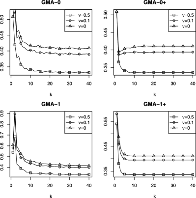
Figure 1: Regrets $R(\mathsf{f}_{\lambda^{(k)}})$ versus iterations $k$ for $\nu=0.5,0.1,0$, under 500 replications.

Figure 1 compares the MSE performance of different values of $\nu$ for greedy algorithms considered in the paper. It shows that for the scenario we are interested in (i.e., where the noise is relatively large, and the best single model is nearly as good as the best convex hull combination), it is beneficial to choose $\nu=0.5$. Note that the greedy procedure with $\nu=0$ converges to the convex hull projection aggregate estimator $\mathsf{f}_{\lambda^{\mathrm{PROJ}}}$ which we have shown to be sub-optimal for MS aggregation. Therefore these results are consistent with our theoretical analysis, and illustrate the importance of $Q$-aggregation with $\nu>0$ for MS aggregation.

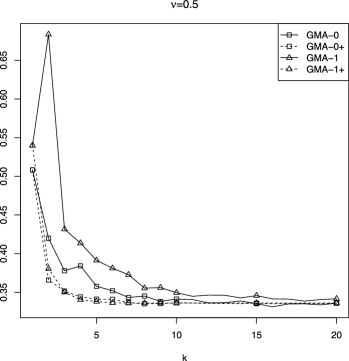
Figure 2: Regrets $R(\mathsf{f}_{\lambda^{(k)}})$ versus iterations $k$ of different greedy procedures at $\nu=0.5$, under 500 replications.

Figure 2 compares the MSE of different greedy procedures at $\nu=0.5$ (additional comparisons at $\nu=0.1$ and $\nu=0$ can be found in Figure 3 in the Appendix B). It shows that the classical first order greedy method GMA-1 generally performs worse than GMA-0 for all $k$ and especially when $k$ is small. This is consistent with our theoretical analysis since Theorem 4.2 only applies to GMA-0. The experiments show that the fully-corrective variants GMA-0₊ and GMA-1₊ can potentially give more accurate results than GMA-0 and GMA-1 at the same sparsity level $k$.

Appendix A Proofs

A.1 Proof of Theorem 4.1

Let $\tilde{\lambda}$ be such that

$$Q(\tilde{\lambda})\leq\min_{\lambda\in\Lambda}\bigl{\{}Q(\lambda)+\varepsilon_{V}V(\lambda)+\varepsilon\bigr{\}}.$$

Fix $\theta\in(0,1)$ and for any $\lambda\in\Lambda$, define ${\lambda_{\theta}}\in\Lambda$ by ${\lambda_{\theta}}=(1-\theta){\tilde{\lambda}}+\theta\lambda$.

Note that

$$P({\tilde{\lambda}})-P({\lambda_{\theta}})=(1-\nu)\bigl{[}\operatorname{MSE}(\mathsf{f}_{\tilde{\lambda}})-\operatorname{MSE}(\mathsf{f}_{{\lambda_{\theta}}})\bigr{]}+\nu\theta\sum_{j=1}^{M}({\tilde{\lambda}}_{j}-\lambda_{j})\operatorname{MSE}(f_{j}).$$

Moreover, it is not hard to verify that

$$\operatorname{MSE}(\mathsf{f}_{\tilde{\lambda}})-\operatorname{MSE}(\mathsf{f}_{{\lambda_{\theta}}})=\theta\operatorname{MSE}(\mathsf{f}_{\tilde{\lambda}})-\theta\operatorname{MSE}(\mathsf{f}_{\lambda})+\theta(1-\theta)\|\mathsf{f}_{\tilde{\lambda}}-\mathsf{f}_{\lambda}\|^{2}.$$

The above two displays and the definition of $P(\lambda)$ yield

$$P({\tilde{\lambda}})-P({\lambda_{\theta}})=\theta\bigl{[}P({\tilde{\lambda}})-P(\lambda)\bigr{]}+\theta(1-\theta)(1-\nu)\|\mathsf{f}_{\tilde{\lambda}}-\mathsf{f}_{\lambda}\|^{2}.$$ (17)

Moreover, by the definition of $\tilde{\lambda}$, we have

$$Q(\tilde{\lambda})\leq Q({\lambda_{\theta}})+\varepsilon_{V}V({\lambda_{\theta}})+\varepsilon.$$

By replacing $Q(\tilde{\lambda})$ and $Q({\lambda_{\theta}})$ with the expansion

$$Q(\lambda)=P(\lambda)+\langle\bolds{\xi},\bolds{\xi}\rangle-2\langle\bolds{\xi},\mathsf{f}_{\lambda}-\eta\rangle+\frac{\beta}{n}\mathcal{K}_{\rho}(\lambda,\pi),$$

where $\bolds{\xi}=\mathbf{Y}-\eta$, we obtain

$$P({\tilde{\lambda}})-P({\lambda_{\theta}}) \leq 2\langle\bolds{\xi},\mathsf{f}_{{\tilde{\lambda}}}-\mathsf{f}_{{\lambda_{\theta}}}\rangle+\frac{\beta}{n}\mathcal{K}_{\rho}({\lambda_{\theta}},\pi)-\frac{\beta}{n}\mathcal{K}_{\rho}({\tilde{\lambda}},\pi)+\varepsilon_{V}V({\lambda_{\theta}})+\varepsilon$$

$$\leq 2\langle\bolds{\xi},\mathsf{f}_{{\tilde{\lambda}}}-\mathsf{f}_{{\lambda_{\theta}}}\rangle+\frac{\beta\theta}{n}\mathcal{K}_{\rho}(\lambda,\pi)-\frac{\beta\theta}{n}\mathcal{K}_{\rho}({\tilde{\lambda}},\pi)+\varepsilon_{V}V({\lambda_{\theta}})+\varepsilon,$$

where in the second inequality, we applied Jensen’s inequality with ${\lambda_{\theta}}=(1-\theta){\tilde{\lambda}}+\theta\lambda$ to the convex function $\lambda\mapsto\mathcal{K}_{\rho}(\lambda,\pi)$. Plugging (17) into this and dividing by $\theta$, we get

$$P({\tilde{\lambda}})-P(\lambda) \leq \tilde{R}_{n}(\mathsf{f}_{\lambda})-(1-\theta)(1-\nu)\|\mathsf{f}_{\tilde{\lambda}}-\mathsf{f}_{\lambda}\|^{2}$$

$${}+\frac{\beta}{n}\mathcal{K}_{\rho}(\lambda,\pi)+\frac{\varepsilon_{V}}{\theta}V({\lambda_{\theta}})+\frac{\varepsilon}{\theta},$$

where, using the fact that $\mathsf{f}_{\tilde{\lambda}}-\mathsf{f}_{{\lambda_{\theta}}}=\theta(\mathsf{f}_{\tilde{\lambda}}-\mathsf{f}_{\lambda})$, we can take

$$\tilde{R}_{n}(\mathsf{f}_{\lambda})=2\langle\bolds{\xi},\mathsf{f}_{{\tilde{\lambda}}}-\mathsf{f}_{\lambda}\rangle-\frac{\beta}{n}\mathcal{K}_{\rho}({\tilde{\lambda}},\pi).$$

The following lemma allows us to control $\tilde{R}_{n}(\mathsf{f}_{\lambda})$ both in expectation and with high probability.

Lemma A.1.

Let the noise vector $\xi=(\xi_{1},\ldots,x_{n})^{\top}$ be sub-Gaussian with variance proxy $\sigma^{2}$. Then, for any $\beta>0$, $\lambda\in\mathbb{R}^{M}$, we have

$$\mathbb{E}\exp\Biggl{(}\frac{n}{\beta}\tilde{R}_{n}(\mathsf{f}_{\lambda})-\frac{2\sigma^{2}n}{\beta^{2}}\sum_{j=1}^{M}{\tilde{\lambda}}_{j}\Upsilon_{j}(\lambda)\Biggr{)}\leq 1,$$

where $\Upsilon_{j}(\lambda)=\|f_{j}-\mathsf{f}_{\lambda}\|^{2}$.

Fix $\lambda\in\mathbb{R}^{M}$. Using successively Jensen’s inequality and the assumption that $t\leq\rho(t)$ yields

$$\mathbb{E}\exp\Biggl{(}\frac{n\tilde{R}_{n}(\mathsf{f}_{\lambda})}{\beta}-\frac{2\sigma^{2}n}{\beta^{2}}\sum_{j=1}^{M}{\tilde{\lambda}}_{j}\Upsilon_{j}(\lambda)\Biggr{)}$$

$$\qquad=\mathbb{E}\exp\Biggl{[}\sum_{j=1}^{M}{\tilde{\lambda}}_{j}\biggl{(}\frac{2n}{\beta}\langle\bolds{\xi},f_{j}-\mathsf{f}_{\lambda}\rangle-\log\biggl{(}\frac{\rho({\tilde{\lambda}}_{j})}{\pi_{j}}\biggr{)}-\frac{2\sigma^{2}n}{\beta^{2}}\Upsilon_{j}(\lambda)\biggr{)}\Biggr{]}$$

$$\qquad\leq\mathbb{E}\sum_{j=1}^{M}{\tilde{\lambda}}_{j}\exp\biggl{(}\frac{2n}{\beta}\langle\bolds{\xi},f_{j}-\mathsf{f}_{\lambda}\rangle-\log\biggl{(}\frac{\rho({\tilde{\lambda}}_{j})}{\pi_{j}}\biggr{)}-\frac{2\sigma^{2}n}{\beta^{2}}\Upsilon_{j}(\lambda)\biggr{)}$$

$$\qquad\leq\sum_{j=1}^{M}\pi_{j}\mathbb{E}\exp\biggl{(}\frac{2n}{\beta}\langle\bolds{\xi},f_{j}-\mathsf{f}_{\lambda}\rangle-\frac{2\sigma^{2}n}{\beta^{2}}\Upsilon_{j}(\lambda)\biggr{)}.$$

Observe now that since $\xi$ is sub-Gaussian, we have

$$\mathbb{E}\exp\biggl{(}\frac{2n}{\beta}\langle\bolds{\xi},f_{j}-\mathsf{f}_{\lambda}\rangle\biggr{)}\leq\exp\biggl{(}\frac{2n\sigma^{2}}{\beta^{2}}\|\mathsf{f}_{\lambda}-f_{j}\|^{2}\biggr{)}=\exp\biggl{(}\frac{2n\sigma^{2}}{\beta^{2}}\Upsilon_{j}(\lambda)\biggr{)}.$$

This completes the proof of our lemma.

To prove the first result of Theorem 4.1, note that Lemma A.1 together with a Chernoff bound yield that for any $\delta\in(0,1)$,

$$\tilde{R}_{n}(\mathsf{f}_{\lambda})\leq\frac{2\sigma^{2}}{\beta}\sum_{j=1}^{M}{\tilde{\lambda}}_{j}\|f_{j}-\mathsf{f}_{\lambda}\|^{2}+\frac{\beta\log(1/\delta)}{n}$$ (19)

with probability at least $1-\delta$. By combining (A.1) and (19), and using the definition of $P({\tilde{\lambda}})$, we obtain

$$(1-\nu)\operatorname{MSE}(\mathsf{f}_{\tilde{\lambda}})+\nu\sum_{j=1}^{M}{\tilde{\lambda}}_{j}\operatorname{MSE}(f_{j})$$

$$\qquad\leq P(\lambda)+\frac{2\sigma^{2}}{\beta}\sum_{j=1}^{M}{\tilde{\lambda}}_{j}\|f_{j}-\mathsf{f}_{\lambda}\|^{2}+\frac{\beta\log(1/\delta)}{n}$$

$$\qquad\quad{}-(1-\theta)(1-\nu)\|\mathsf{f}_{\tilde{\lambda}}-\mathsf{f}_{\lambda}\|^{2}+\frac{\beta}{n}\mathcal{K}_{\rho}(\lambda,\pi)+\frac{\varepsilon_{V}}{\theta}V({\lambda_{\theta}})+\frac{\varepsilon}{\theta}.$$

The following identities follows directly from algebra:

$$\sum_{j=1}^{M}{\tilde{\lambda}}_{j}\operatorname{MSE}(f_{j}) = \operatorname{MSE}(\mathsf{f}_{{\tilde{\lambda}}})+V({\tilde{\lambda}}),$$

$$\sum_{j=1}^{M}{\tilde{\lambda}}_{j}\|f_{j}-\mathsf{f}_{\lambda}\|^{2} = V({\tilde{\lambda}})+\|\mathsf{f}_{{\tilde{\lambda}}}-\mathsf{f}_{\lambda}\|^{2}.$$

Together with (A.1), they yield

$$\operatorname{MSE}(\mathsf{f}_{\tilde{\lambda}}) \leq P(\lambda)+\biggl{(}\frac{2\sigma^{2}}{\beta}-\nu\biggr{)}V({\tilde{\lambda}})+\frac{\beta\log(1/\delta)}{n}$$

$${}+\biggl{[}\frac{2\sigma^{2}}{\beta}-(1-\theta)(1-\nu)\biggr{]}\|\mathsf{f}_{\tilde{\lambda}}-\mathsf{f}_{\lambda}\|^{2}+\frac{\beta}{n}\mathcal{K}_{\rho}(\lambda,\pi)$$

$${}+\frac{\varepsilon_{V}}{\theta}V({\lambda_{\theta}})+\frac{\varepsilon}{\theta}.$$

We now use the following identity which again follows directly from algebra:

$$V({\lambda_{\theta}})=\theta V(\lambda)+(1-\theta)V({\tilde{\lambda}})+\theta(1-\theta)\|\mathsf{f}_{{\tilde{\lambda}}}-\mathsf{f}_{\lambda}\|^{2}.$$

Together with (A.1), we obtain

$$\operatorname{MSE}(\mathsf{f}_{{\tilde{\lambda}}})\leq P(\lambda)+G_{1}V({\tilde{\lambda}})+G_{2}\|\mathsf{f}_{\tilde{\lambda}}-\mathsf{f}_{\lambda}\|^{2}+\frac{\beta}{n}\mathcal{K}_{\rho}(\lambda,\delta\pi)+\varepsilon_{V}V(\lambda)+\frac{\varepsilon}{\theta},$$

where $\delta\pi=(\delta\pi_{1},\ldots,\delta\pi_{M})^{\top}$,

$$G_{1}=\frac{2\sigma^{2}}{\beta}-\nu+\frac{\varepsilon_{V}(1-\theta)}{\theta}$$

and

$$G_{2}=\frac{2\sigma^{2}}{\beta}-(1-\theta)(1-\nu)+\varepsilon_{V}(1-\theta).$$

To complete the proof of (15), it is sufficient to note that choosing $\beta$ as in (14) ensures that $G_{1}\leq 0$ and $G_{2}\leq 0$.

Using the convexity inequality $t\leq e^{t}-1$ for any $t\in\mathbb{R}$, it yields that (19) also holds in expectation. The proof of (16) is then concluded in the same way as the proof of (15) by making statements in expectation instead of statements that hold with high probability.

A.2 Proof of Theorem 4.2

It follows from a Taylor expansion that for any $\mu,\mu^{\prime}\in\Lambda$, we have

$$Q(\mu)=Q\bigl{(}\mu^{\prime}\bigr{)}+\bigl{(}\mu-\mu^{\prime}\bigr{)}^{\top}\nabla Q\bigl{(}\mu^{\prime}\bigr{)}+(1-\nu)\|\mathsf{f}_{\mu}-\mathsf{f}_{\mu^{\prime}}\|^{2}.$$ (22)

Observe also that for any $\lambda\in\Lambda$, we have (both for GMA-0 and GMA-0₊)

$$Q\bigl{(}\lambda^{(k+1)}\bigr{)}\leq\sum_{j=1}^{M}\lambda_{j}Q\bigl{(}\lambda^{(k)}+\alpha_{k+1}\bigl{(}\mathsf{e}^{(j)}-\lambda^{(k)}\bigr{)}\bigr{)}.$$

Expanding each term on the right-hand side using (22) with $\mu=\lambda^{(k)}+\alpha_{k+1}(\mathsf{e}^{(j)}-\lambda^{(k)})$ and $\mu^{\prime}=\lambda^{(k)}$ yields

$$Q\bigl{(}\lambda^{(k+1)}\bigr{)} \leq Q\bigl{(}\lambda^{(k)}\bigr{)}+\alpha_{k+1}^{2}(1-\nu)\sum_{j=1}^{M}\lambda_{j}\|f_{j}-\mathsf{f}_{\lambda^{(k)}}\|^{2}$$

$${}+\alpha_{k+1}\bigl{(}\lambda-\lambda^{(k)}\bigr{)}^{\top}\nabla Q\bigl{(}\lambda^{(k)}\bigr{)}.$$

Note that

$$\sum_{j=1}^{M}\lambda_{j}\|f_{j}-\mathsf{f}_{\lambda^{(k)}}\|^{2}=\sum_{j=1}^{M}\lambda_{j}\|f_{j}-\mathsf{f}_{\lambda}\|^{2}+\|\mathsf{f}_{\lambda^{(k)}}-\mathsf{f}_{\lambda}\|^{2}.$$

Moreover, applying (22) with $\mu=\lambda$ and $\mu^{\prime}=\lambda^{(k)}$ yields

$$\alpha_{k+1}\bigl{(}\lambda-\lambda^{(k)}\bigr{)}^{\top}\nabla Q\bigl{(}\lambda^{(k)}\bigr{)}=\alpha_{k+1}\bigl{[}Q(\lambda)-Q\bigl{(}\lambda^{(k)}\bigr{)}\bigr{]}-(1-\nu)\alpha_{k+1}\|\mathsf{f}_{\lambda^{(k)}}-\mathsf{f}_{\lambda}\|^{2}.$$

Plugging the above two displays into (A.2) and using $\alpha_{k+1}^{2}-\alpha_{k+1}\leq 0$, we get

$$Q\bigl{(}\lambda^{(k+1)}\bigr{)}\leq Q\bigl{(}\lambda^{(k)}\bigr{)}+\alpha_{k+1}^{2}(1-\nu)\sum_{j=1}^{M}\lambda_{j}\|f_{j}-\mathsf{f}_{\lambda}\|^{2}+\alpha_{k+1}\bigl{[}Q(\lambda)-Q\bigl{(}\lambda^{(k)}\bigr{)}\bigr{]}.$$

This can be written as

$$\delta_{k+1}\leq(1-\alpha_{k+1})\delta_{k}+\alpha_{k+1}^{2}B,$$ (24)

where

$$\delta_{k}=Q\bigl{(}\lambda^{(k)}\bigr{)}-Q(\lambda),\qquad B=(1-\nu)\sum_{j=1}^{M}\lambda_{j}\|f_{j}-\mathsf{f}_{\lambda}\|^{2}.$$

To conclude that

$$\delta_{k}\leq\frac{4B}{k+3},$$ (25)

we proceed by induction on $k$. It is easy to see from (24) with $k=0$ and $\alpha_{1}=1$ that $\delta_{1}\leq B$.

Now for $k\geq 1$, bound (24) yields

$$\delta_{k+1} \leq \biggl{(}1-\frac{2}{2+k}\biggr{)}\delta_{k}+\biggl{(}\frac{2}{2+k}\biggr{)}^{2}B$$

$$\leq \biggl{(}1-\frac{2}{2+k}\biggr{)}\frac{4B}{k+3}+\biggl{(}\frac{2}{2+k}\biggr{)}^{2}B=\frac{4(k^{2}+3k+3)B}{(k+2)^{2}(k+3)}\leq\frac{4B}{k+4},$$

where in the second inequality, we used (25). We have proved that for any $\lambda$, it holds

$$Q\bigl{(}\lambda^{(k)}\bigr{)}\leq Q(\lambda)+\frac{4(1-\nu)}{k+3}\sum_{j=1}^{M}\lambda_{j}\|f_{j}-\mathsf{f}_{\lambda}\|^{2}.$$

To complete the proof, we check that the assumptions of Theorem 4.1 with $\varepsilon_{V}=4(1-\nu)/(k+3)$ and $\varepsilon=0$ are satisfied. Moreover, using expression (14), we get the desired bound on $\beta$. To conclude, notice that $V(\lambda)$ vanishes at the vertices of the simplex $\Lambda$.

A.3 Proof of Proposition 4.1

Similarly to the proof of Theorem 4.2, for both GMA-1 and GMA-1₊, we have

$$Q\bigl{(}\lambda^{(k+1)}\bigr{)}-(1-\nu)\alpha_{k+1}^{2}\|f_{J^{(k)}}-\mathsf{f}_{\lambda^{(k)}}\|^{2}$$

$$\qquad=Q\bigl{(}\lambda^{(k)}\bigr{)}+\alpha_{k+1}\bigl{(}\mathsf{e}^{(J^{(k)})}-\lambda^{(k)}\bigr{)}^{\top}\nabla Q\bigl{(}\lambda^{(k)}\bigr{)}$$

$$\qquad\leq\sum_{j=1}^{M}\lambda_{j}\bigl{[}Q\bigl{(}\lambda^{(k)}\bigr{)}+\alpha_{k+1}\bigl{(}\mathsf{e}^{(j)}-\lambda^{(k)}\bigr{)}^{\top}\nabla Q\bigl{(}\lambda^{(k)}\bigr{)}\bigr{]}$$

$$\qquad=Q\bigl{(}\lambda^{(k)}\bigr{)}+\alpha_{k+1}\nabla Q\bigl{(}\lambda^{(k)}\bigr{)}^{\top}\bigl{(}\lambda-\lambda^{(k)}\bigr{)}$$

$$\qquad=Q\bigl{(}\lambda^{(k)}\bigr{)}+\alpha_{k+1}\bigl{[}Q(\lambda)-Q\bigl{(}\lambda^{(k)}\bigr{)}-(1-\nu)\|\mathsf{f}_{\lambda}-\mathsf{f}_{\lambda^{(k)}}\|^{2}\bigr{]}.$$

Using $\|f_{J^{(k)}}-\mathsf{f}_{\lambda^{(k)}}\|^{2}\leq 4L^{2}$, we obtain

$$\delta_{k+1}\leq(1-\alpha_{k+1})\delta_{k}+\alpha_{k+1}^{2}B^{\prime},$$ (26)

where we define

$$\delta_{k}=Q\bigl{(}\lambda^{(k)}\bigr{)}-Q(\lambda),\qquad B^{\prime}=4(1-\nu)L^{2}.$$

Note that (26) also holds for GMA-0 and GMA-0₊ due to (24). Therefore similarly to the proof of Theorem 4.2, we can solve the recursion in (26) to obtain

$$\delta_{k}\leq\frac{4B^{\prime}}{k+3}=\frac{16(1-\nu)L^{2}}{k+3}.$$

That is, we have

$$Q\bigl{(}\lambda^{(k)}\bigr{)}\leq\min_{\lambda\in\Lambda}Q(\lambda)+\frac{16(1-\nu)L^{2}}{k+3}.$$

We can thus apply Theorem 4.1 with $\varepsilon_{V}=0$, $\varepsilon=16(1-\nu)L^{2}/(k+3)$, and $\theta=(1-2\nu)/(1-\nu)$ to complete the proof.

Table 2: Regret of different algorithms: oracle model is superior to averaged models

STAR	EXP	PROJ
$0.43\pm 0.41$	$0.386\pm 0.47$	$0.407\pm 0.28$

	$\bolds{k=1}$	$\bolds{k=2}$	$\bolds{k=5}$	$\bolds{k=20}$	$\bolds{k=40}$
GMA-0
$\nu=0.5$	$0.508\pm 0.76$	$0.42\pm 0.53$	$0.358\pm 0.42$	$0.336\pm 0.38$	$0.332\pm 0.37$
$\nu=0.1$	$0.508\pm 0.76$	$0.523\pm 0.5$	$0.424\pm 0.35$	$0.394\pm 0.3$	$0.389\pm 0.3$
$\nu=0$	$0.508\pm 0.76$	$0.55\pm 0.48$	$0.444\pm 0.34$	$0.411\pm 0.29$	$0.409\pm 0.28$
GMA-0+
$\nu=0.5$	$0.508\pm 0.76$	$0.366\pm 0.5$	$0.341\pm 0.4$	$0.336\pm 0.38$	$0.336\pm 0.38$
$\nu=0.1$	$0.508\pm 0.76$	$0.387\pm 0.44$	$0.391\pm 0.33$	$0.394\pm 0.3$	$0.394\pm 0.3$
$\nu=0$	$0.508\pm 0.76$	$0.396\pm 0.43$	$0.403\pm 0.32$	$0.411\pm 0.29$	$0.411\pm 0.29$
GMA-1
$\nu=0.5$	$0.54\pm 0.79$	$0.683\pm 0.44$	$0.391\pm 0.38$	$0.342\pm 0.36$	$0.334\pm 0.37$
$\nu=0.1$	$0.58\pm 0.83$	$0.897\pm 0.35$	$0.49\pm 0.31$	$0.41\pm 0.29$	$0.399\pm 0.29$
$\nu=0$	$0.609\pm 0.84$	$0.937\pm 0.32$	$0.528\pm 0.3$	$0.428\pm 0.27$	$0.415\pm 0.28$
GMA-1+
$\nu=0.5$	$0.54\pm 0.79$	$0.381\pm 0.46$	$0.338\pm 0.38$	$0.336\pm 0.38$	$0.336\pm 0.38$
$\nu=0.1$	$0.58\pm 0.83$	$0.459\pm 0.45$	$0.4\pm 0.31$	$0.395\pm 0.3$	$0.395\pm 0.3$
$\nu=0$	$0.609\pm 0.84$	$0.488\pm 0.45$	$0.418\pm 0.3$	$0.411\pm 0.29$	$0.411\pm 0.29$

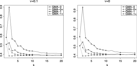
Figure 3: Regrets $R(\mathsf{f}_{\lambda^{(k)}})$ versus iterations $k$ of different greedy procedures at $\nu=0.1$ and $\nu=0$, under 500 replications.

Appendix B Detailed Performance Table and Figures

Acknowledgment

We would like to thank an anonymous referee for suggesting an improvement of bound (14).

References

- Audibert (2004) {barticle}[mr] \bauthor\bsnmAudibert, \bfnmJean-Yves\binitsJ.-Y. (\byear2004). \btitleAggregated estimators and empirical complexity for least square regression. \bjournalAnn. Inst. Henri Poincaré Probab. Stat. \bvolume40 \bpages685–736. \biddoi=10.1016/j.anihpb.2003.11.006, issn=0246-0203, mr=2096215 \bptokimsref \endbibitem
- Audibert (2008) {bincollection}[author] \bauthor\bsnmAudibert, \bfnmJean-Yves\binitsJ.-Y. (\byear2008). \btitleProgressive mixture rules are deviation suboptimal. In \bbooktitleAdvances in Neural Information Processing Systems 20 (\beditor\bfnmJ. C.\binitsJ. C. \bsnmPlatt, \beditor\bfnmD.\binitsD. \bsnmKoller, \beditor\bfnmY.\binitsY. \bsnmSinger and \beditor\bfnmS.\binitsS. \bsnmRoweis, eds.) \bpages41–48. \bpublisherMIT Press, \baddressCambridge, MA. \bptokimsref \endbibitem
- Barron (1993) {barticle}[mr] \bauthor\bsnmBarron, \bfnmAndrew R.\binitsA. R. (\byear1993). \btitleUniversal approximation bounds for superpositions of a sigmoidal function. \bjournalIEEE Trans. Inform. Theory \bvolume39 \bpages930–945. \biddoi=10.1109/18.256500, issn=0018-9448, mr=1237720 \bptokimsref \endbibitem
- Beck and Teboulle (2009) {barticle}[mr] \bauthor\bsnmBeck, \bfnmAmir\binitsA. and \bauthor\bsnmTeboulle, \bfnmMarc\binitsM. (\byear2009). \btitleA fast iterative shrinkage-thresholding algorithm for linear inverse problems. \bjournalSIAM J. Imaging Sci. \bvolume2 \bpages183–202. \biddoi=10.1137/080716542, issn=1936-4954, mr=2486527 \bptokimsref \endbibitem
- Boyd and Vandenberghe (2004) {bbook}[mr] \bauthor\bsnmBoyd, \bfnmStephen\binitsS. and \bauthor\bsnmVandenberghe, \bfnmLieven\binitsL. (\byear2004). \btitleConvex Optimization. \bpublisherCambridge Univ. Press, \baddressCambridge. \bidmr=2061575 \bptokimsref \endbibitem
- Catoni (1999) {bmisc}[author] \bauthor\bsnmCatoni, \bfnmO.\binitsO. (\byear1999). \bhowpublishedUniversal aggregation rules with exact bias bounds. Technical report, Laboratoire de Probabilités et Modeles Aléatoires, Paris. \bptokimsref \endbibitem
- Clarkson (2008) {binproceedings}[mr] \bauthor\bsnmClarkson, \bfnmKenneth L.\binitsK. L. (\byear2008). \btitleCoresets, sparse greedy approximation, and the Frank–Wolfe algorithm. In \bbooktitleProceedings of the Nineteenth Annual ACM-SIAM Symposium on Discrete Algorithms \bpages922–931. \bpublisherACM, \baddressNew York. \bidmr=2487663 \bptokimsref \endbibitem
- Dai and Zhang (2011) {bincollection}[author] \bauthor\bsnmDai, \bfnmDong\binitsD. and \bauthor\bsnmZhang, \bfnmTong\binitsT. (\byear2011). \btitleGreedy model averaging. In \bbooktitleAdvances in Neural Information Processing Systems 24 (\beditor\bfnmJ.\binitsJ. \bsnmShawe-Taylor, \beditor\bfnmR. S.\binitsR. S. \bsnmZemel, \beditor\bfnmP.\binitsP. \bsnmBartlett, \beditor\bfnmF. C. N.\binitsF. C. N. \bsnmPereira and \beditor\bfnmK. Q.\binitsK. Q. \bsnmWeinberger, eds.) \bpages1242–1250. \bpublisherMIT Press, \baddressCambridge, MA. \bptokimsref \endbibitem
- Dalalyan and Salmon (2011) {bmisc}[author] \bauthor\bsnmDalalyan, \bfnmA. S.\binitsA. S. and \bauthor\bsnmSalmon, \bfnmJ.\binitsJ. (\byear2011). \bhowpublishedSharp oracle inequalities for aggregation of affine estimators. Available at arXiv:\arxivurl1104.3969. \bptokimsref \endbibitem
- Dalalyan and Tsybakov (2007) {bincollection}[mr] \bauthor\bsnmDalalyan, \bfnmArnak S.\binitsA. S. and \bauthor\bsnmTsybakov, \bfnmAlexandre B.\binitsA. B. (\byear2007). \btitleAggregation by exponential weighting and sharp oracle inequalities. In \bbooktitleLearning Theory. \bseriesLecture Notes in Computer Science \bvolume4539 \bpages97–111. \bpublisherSpringer, \baddressBerlin. \biddoi=10.1007/978-3-540-72927-3_9, mr=2397581 \bptokimsref \endbibitem
- Dalalyan and Tsybakov (2008) {barticle}[author] \bauthor\bsnmDalalyan, \bfnmA.\binitsA. and \bauthor\bsnmTsybakov, \bfnmA. B.\binitsA. B. (\byear2008). \btitleAggregation by exponential weighting, sharp PAC-Bayesian bounds and sparsity. \bjournalMachine Learning \bvolume72 \bpages39–61. \bptokimsref \endbibitem
- Frank and Wolfe (1956) {barticle}[mr] \bauthor\bsnmFrank, \bfnmMarguerite\binitsM. and \bauthor\bsnmWolfe, \bfnmPhilip\binitsP. (\byear1956). \btitleAn algorithm for quadratic programming. \bjournalNaval Res. Logist. Quart. \bvolume3 \bpages95–110. \bidissn=0028-1441, mr=0089102 \bptokimsref \endbibitem
- Gaïffas and Lecué (2011) {barticle}[mr] \bauthor\bsnmGaïffas, \bfnmStéphane\binitsS. and \bauthor\bsnmLecué, \bfnmGuillaume\binitsG. (\byear2011). \btitleHyper-sparse optimal aggregation. \bjournalJ. Mach. Learn. Res. \bvolume12 \bpages1813–1833. \bidissn=1532-4435, mr=2819018 \bptokimsref \endbibitem
- Jaggi (2011) {bmisc}[author] \bauthor\bsnmJaggi, \bfnmMartin\binitsM. (\byear2011). \bhowpublishedConvex optimization without projection steps. Available at arXiv:\arxivurl1108.1170v6. \bptokimsref \endbibitem
- Jones (1992) {barticle}[mr] \bauthor\bsnmJones, \bfnmLee K.\binitsL. K. (\byear1992). \btitleA simple lemma on greedy approximation in Hilbert space and convergence rates for projection pursuit regression and neural network training. \bjournalAnn. Statist. \bvolume20 \bpages608–613. \biddoi=10.1214/aos/1176348546, issn=0090-5364, mr=1150368 \bptokimsref \endbibitem
- Juditsky and Nemirovski (2000) {barticle}[mr] \bauthor\bsnmJuditsky, \bfnmAnatoli\binitsA. and \bauthor\bsnmNemirovski, \bfnmArkadii\binitsA. (\byear2000). \btitleFunctional aggregation for nonparametric regression. \bjournalAnn. Statist. \bvolume28 \bpages681–712. \biddoi=10.1214/aos/1015951994, issn=0090-5364, mr=1792783 \bptokimsref \endbibitem
- Juditsky, Rigollet and Tsybakov (2008) {barticle}[mr] \bauthor\bsnmJuditsky, \bfnmA.\binitsA., \bauthor\bsnmRigollet, \bfnmP.\binitsP. and \bauthor\bsnmTsybakov, \bfnmA. B.\binitsA. B. (\byear2008). \btitleLearning by mirror averaging. \bjournalAnn. Statist. \bvolume36 \bpages2183–2206. \biddoi=10.1214/07-AOS546, issn=0090-5364, mr=2458184 \bptokimsref \endbibitem
- Laurent and Massart (2000) {barticle}[mr] \bauthor\bsnmLaurent, \bfnmB.\binitsB. and \bauthor\bsnmMassart, \bfnmP.\binitsP. (\byear2000). \btitleAdaptive estimation of a quadratic functional by model selection. \bjournalAnn. Statist. \bvolume28 \bpages1302–1338. \biddoi=10.1214/aos/1015957395, issn=0090-5364, mr=1805785 \bptokimsref \endbibitem
- Lecué and Mendelson (2009) {barticle}[mr] \bauthor\bsnmLecué, \bfnmGuillaume\binitsG. and \bauthor\bsnmMendelson, \bfnmShahar\binitsS. (\byear2009). \btitleAggregation via empirical risk minimization. \bjournalProbab. Theory Related Fields \bvolume145 \bpages591–613. \biddoi=10.1007/s00440-008-0180-8, issn=0178-8051, mr=2529440 \bptokimsref \endbibitem
- Lecué and Mendelson (2012) {bmisc}[author] \bauthor\bsnmLecué, \bfnmGuillaume\binitsG. and \bauthor\bsnmMendelson, \bfnmShahar\binitsS. (\byear2012). \bhowpublishedOn the optimality of the aggregate with exponential weights for low temperatures. Bernoulli. To appear. \bptokimsref \endbibitem
- Nemirovski (2000) {bincollection}[mr] \bauthor\bsnmNemirovski, \bfnmArkadi\binitsA. (\byear2000). \btitleTopics in non-parametric statistics. In \bbooktitleLectures on Probability Theory and Statistics (Saint-Flour, 1998). \bseriesLecture Notes in Math. \bvolume1738 \bpages85–277. \bpublisherSpringer, \baddressBerlin. \bidmr=1775640 \bptokimsref \endbibitem
- Rigollet (2012) {barticle}[author] \bauthor\bsnmRigollet, \bfnmPhilippe\binitsP. (\byear2012). \btitleKullback–Leibler aggregation and misspecified generalized linear models. \bjournalAnn. Statist. \bvolume40 \bpages639–665. \bptokimsref \endbibitem
- Rigollet and Tsybakov (2011) {barticle}[mr] \bauthor\bsnmRigollet, \bfnmPhilippe\binitsP. and \bauthor\bsnmTsybakov, \bfnmAlexandre\binitsA. (\byear2011). \btitleExponential screening and optimal rates of sparse estimation. \bjournalAnn. Statist. \bvolume39 \bpages731–771. \biddoi=10.1214/10-AOS854, issn=0090-5364, mr=2816337 \bptokimsref \endbibitem
- Rigollet and Tsybakov (2012) {bmisc}[author] \bauthor\bsnmRigollet, \bfnmP.\binitsP. and \bauthor\bsnmTsybakov, \bfnmA.\binitsA. (\byear2012). \bhowpublishedSparse estimation by exponential weighting. Statist. Sci. To appear. Available at arXiv:\arxivurl1108.5116. \bptokimsref \endbibitem
- Shalev-Shwartz, Srebro and Zhang (2010) {barticle}[mr] \bauthor\bsnmShalev-Shwartz, \bfnmShai\binitsS., \bauthor\bsnmSrebro, \bfnmNathan\binitsN. and \bauthor\bsnmZhang, \bfnmTong\binitsT. (\byear2010). \btitleTrading accuracy for sparsity in optimization problems with sparsity constraints. \bjournalSIAM J. Optim. \bvolume20 \bpages2807–2832. \biddoi=10.1137/090759574, issn=1052-6234, mr=2721156 \bptokimsref \endbibitem
- Tsybakov (2003) {binproceedings}[author] \bauthor\bsnmTsybakov, \bfnmAlexandre B.\binitsA. B. (\byear2003). \btitleOptimal rates of aggregation. In \bbooktitleCOLT (\beditor\bfnmBernhard\binitsB. \bsnmSchölkopf and \beditor\bfnmManfred K.\binitsM. K. \bsnmWarmuth, eds.). \bseriesLecture Notes in Computer Science \bvolume2777 \bpages303–313. \bpublisherSpringer, \baddressBerlin. \bptokimsref \endbibitem
- Yang (1999) {barticle}[mr] \bauthor\bsnmYang, \bfnmYuhong\binitsY. (\byear1999). \btitleModel selection for nonparametric regression. \bjournalStatist. Sinica \bvolume9 \bpages475–499. \bidissn=1017-0405, mr=1707850 \bptokimsref \endbibitem