Valley-kink in Bilayer Graphene at $\nu=0$: A Charge Density Signature for Quantum Hall Ferromagnetism

Abstract

We investigate interaction-induced valley domain walls in bilayer graphene in the $\nu=0$ quantum Hall state, subject to a perpendicular electric field that is antisymmetric across a line in the sample. Such a state can be realized in a double-gated suspended sample, where the electric field changes sign across a line in the middle. The non-interacting energy spectrum of the ground state is characterized by a sharp domain wall between two valley-polarized regions. Using the Hartree-Fock approximation, we find that the Coulomb interaction opens a gap between the two lowest-lying states near the Fermi level, yielding a smooth domain wall with a kink configuration in the valley index. Our results suggest the possibility to visualize the domain wall via measuring the charge density difference between the two graphene layers, which we find exhibits a characteristic pattern. The width of the kink and the resulting pattern can be tuned by the interplay between the magnetic field and gate electric fields.

I Introduction

Two dimensional electron systems in magnetic fields exhibit a great richness of physics, particularly in the high field regime where the decreasing radius of the cyclotron orbits gives rise to increasing importance of electron-electron interactions. Two examples are the fractional quantum Hall effect (FQHE) and quantum Hall ferromagnets in the integer QHE.Sarma and Pinczuk (1997); Prange and Girvin (1990) The essential feature of the former is a condensation of the electrons into unusual correlated states which minimize the Coulomb energy, allowing the electrons to avoid each other as much as possible. Similarly, for the latter, Coulomb interactions induce nonperturbative effects on the highly degenerate Landau bands of the non-interacting system. In particular, due to exchange, ferromagnetism is induced in the system. A prominent manifestation of this state is the formation of Skyrmions as novel low energy excitations of the spin-polarized ground state (or isospin polarized states in bilayer QH systems).Prange and Girvin (1990); Sarma and Pinczuk (1997); Sondhi et al. (1993); Fertig et al. (1994); Moon et al. (1995)

Quantum Hall ferromagnets have also been predicted for graphene in the integer quantum Hall regimes,Abanin et al. (2007); Bolotin et al. (2009); Du et al. (2009); Fertig and Brey (2006); Zhao et al. (2010); Barlas et al. (2008); Cote et al. (2008) which exhibit particle-hole conjugate Landau levels and a peculiar $\nu=0$ QH state at zero energy.Novoselov et al. (2005, 2006); Zhang et al. (2005); Zheng and Ando (2002) These two unique features are manifestations of the Dirac equation which governs the electron dynamics near the $\mathbf{K}$ and $\mathbf{K^{\prime}}$ points in the band structure. For non-interacting electrons in graphene, four Landau levels are present near zero energy, associated with the two valleys and the two spin states. In this situation the Zeeman coupling separates the states into two pairs above and below the Fermi energy. When interactions are included, the half-filled zero energy states spontaneously polarize due to exchange and give rise to a ferromagnetic ground state,Sarma and Pinczuk (1997) which may be spin or valley polarized depending on the strength of the field.Zhang et al. (2006); Zhao et al. (2012)

In addition to this interesting bulk property in the $\nu=0$ state, a coherent domain wallFertig and Brey (2006); Shimshoni et al. (2009) (DW) will be present between a spin polarized bulk state and an unpolarized region at the physical edge of a finite graphene ribbon.Castro Neto et al. (2006); Brey and Fertig (2006) This DW has also been predicted to support a Luttinger liquid edge mode, which is another manifestation of the Coulomb interaction in 2D systems. However, it may be difficult to realize this spin configuration in currently available graphene ribbons, as their edges are in general rough.Li et al. (2011) Moreover, such a pattern in the ground state is hard to probe directly.

An “internal edge” in biased bilayer graphene (BLG) proposed by Martin $\mathit{et\>}al.$ provides an alternative way to create a DW that circumvents the difficulty in making perfect physical edges.Martin et al. (2008); Zarenia et al. (2011) This clean edge can be created in the middle of a bilayer graphene sample by placing it in an electric quadrupole gate where a potential profile changes sign across the center of the sample, as shown in Fig. 1. When the Fermi level is placed at zero energy, a pair of surface states with opposite chiralities and opposite isospins (valley index) are formed in the middle of the sample. These states are localized and resemble the edge states of quantum Hall systems near a physical edge.

In the QH regime, bilayer graphene also exhibits particle-hole symmetric LLs and particle-hole degenerate zero energy states. Relative to the monolayer, the layer degrees of freedom of the bilayer system doubles the zero energy degeneracy. Perpendicular electric fields act as Zeeman fields for the layer degrees of freedom,McCann and Falko (2006); McCann (2006) thus lifting their degeneracy. This effective Zeeman field can be tuned to be much larger than the Zeeman splitting of the real spin, set by the magnetic field. In the double-gated setting, this isospin Zeeman splitting changes sign in the middle of the sample, yielding level crossings similar to the physical edge of a monolayer graphene sample. When interactions are included, QH ferromagnetism sets in and the fully polarized ground state acquires a finite spin stiffness. As a result, a coherent DW analogous to the spin DW found in Ref. Fertig and Brey, 2006 may form.

In this paper, we study the interaction-induced valley DW in bilayer graphene in the $\nu=0$ quantum Hall state, in a physical configuration as shown in Fig. 1. The perpendicular magnetic field $B_{z}$, the strength of the perpendicular bias $E_{z}$, and the separation of two electric gates are controllable parameters. We use the Hartree-Fock approximation to derive the ground state and to evaluate the width of the DW in terms of these parameters. We find that the DW has an interlayer charge density difference pattern, which may be accessible experimentally.

This paper is organized as follows. In Section II, we review the non-interacting energy spectrum of bilayer graphene with Bernal stacking under a perpendicular magnetic field and a double gated bias with different polarities. In Section III, we derive the ground state wavefunction and energy of the valley-kink domain wall within a self-consistent Hartree-Fock approximation, and evaluate the size of the coherent domain wall. Section IV discusses the resulting charge density pattern. Finally, we summarize our results and discuss future directions in Section V.

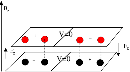
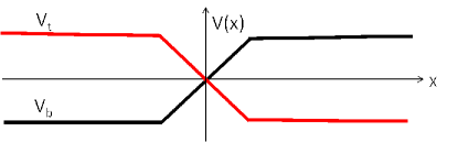
Figure 1: (Color online) Bilayer graphene in a double gated system. Upper panel: the red dot ($B$) represents the sublattice $B$ on the top layer, and the black dot ($\tilde{A}$) represents the sublattice $A$ on the bottom layer of a BLG. The imaginary line connecting the $\tilde{A}B$ dimmer represents $\gamma_{1}$ bonding. The polarities are different on the two sides of the system. Lower panel: $V_{t}$ marked by red solid line represents the potential profile for top layer, and $V_{b}$ marked by black solid line represents the potential profile for the bottom layer. Here we assume an adiabatic linear profile across the middle of the sample.

II Non-interacting model

We consider a bilayer graphene sheet subject to a perpendicular electric field which varies along the $x$ direction as shown in Fig. 1. With a gauge choice of $\mathbf{A}=\widehat{y}xB_{z}$ for the magnetic vector potential, the electron wavefunctions are localized in the $x$ direction and extended along the $y$ direction with a good quantum number $k_{y}$. When the Zeeman splitting is small, the low-energy Hamiltonian of biased bilayer graphene with Bernal stacking in the vicinity of the $\mathbf{K}$ valley isMartin et al. (2008); Mazo et al. (2011)

$$H_{\mathbf{K}}=\left(\begin{array}[]{cccc}-V(x)/2&\omega_{c}a&0&0\\ \omega_{c}a^{\dagger}&-V(x)/2&\gamma_{1}&0\\ 0&\gamma_{1}&V(x)/2&\omega_{c}a\\ 0&0&\omega_{c}a^{\dagger}&V(x)/2\end{array}\right),$$ (1)

where the basis for the Hamiltonian is $\left(\tilde{\left\langle B\right|},\tilde{\left\langle A\right|},\left\langle B\right|,\left\langle A\right|\right)^{{\dagger}}$, and $A$, $B$ ($\tilde{A}$, $\tilde{B}$) represent the sublattice wavefunctions on the top and bottom layer respectively. Here $a=\left[\partial_{x}+(x-X)\right]/\sqrt{2}$ and $a^{\dagger}=\left[-\partial_{x}+(x-X)\right]/\sqrt{2}$, where $x$ (and all length scales henceforth) is in units of the magnetic length $l_{B}$, the guiding center is defined as $X=l_{B}k_{y}$, and $\omega_{c}=\sqrt{2}\hbar v_{F}/l_{B}$ $(v_{F}\thickapprox 10^{6}ms^{-1})$.Castro Neto et al. (2009); Wallace (1947) The dominant interlayer coupling constant ($\gamma_{1}\sim 0.3$ eV) included in the model is between the $\tilde{A}B$ dimer sites. $V(x)$ is the interlayer bias, assumed to be adiabatically varied so that in the effective Hamiltonian for a given $x$, $V(x)$ may be replaced by $V(X)$. For simplicity, we consider

$$V(X) = \begin{cases}-V,&X<-w/2\\ \left(\frac{V}{w}\right)X,&-w/2<X<w/2\\ V,&X>w/2\end{cases},$$ (2)

where $w$ defines the separation of the two electric gates with opposite polarities, assumed to be much larger than $l_{B}$. The two lowest lying eigenvalues are

$$\varepsilon_{1}^{\mathbf{K}}=\frac{V(X)}{2}$$ (3)

and

$$\varepsilon_{2}^{\mathbf{K}}=\frac{\gamma_{1}^{2}-\omega_{c}^{2}}{2\left(\gamma_{1}^{2}+\omega_{c}^{2}\right)}V(X),$$ (4)

and their corresponding eigenstates are

$$\phi_{1,\mathbf{K}X}(\mathbf{r})=\frac{e^{i\left(K+X\right)y}}{\sqrt{L_{y}}}\left(\begin{array}[]{c}0\\ 0\\ 0\\ \Phi_{0}(x-X)\end{array}\right),$$ (5)

$$\phi_{2,\mathbf{K}X}(\mathbf{r})=\frac{e^{i\left(K+X\right)y}}{\sqrt{L_{y}}N_{h}}\left(\begin{array}[]{c}0\\ \Phi_{0}(x-X)\\ \frac{\gamma_{1}V(X)}{\gamma_{1}^{2}+\omega_{c}^{2}}\Phi_{0}(x-X)\\ -\frac{\gamma_{1}}{\omega_{c}}\Phi_{1}(x-X)\end{array}\right),$$ (6)

where $\Phi_{n}(x-X)$ are the harmonic oscillator wavefunctions and $N_{h}$ is a normalization factor. The $\phi_{1}$ state is purely from the lowest Landau level (LLL) of the top layer, while the $\phi_{2}$ state consists of the LLL from the bottom layer and the first LL from the top layer. Their distinction will be clear when we calculate the exchange energies. The representation of the Hamiltonian in $\mathbb{\mathbf{K^{\prime}}}$ has the same form with $V(X)\rightarrow-V(X)$, and a basis where the order of components in the 4-spinor is inverted, hence $\varepsilon_{i}^{\mathbf{K^{\prime}}}(X)=-\varepsilon_{i}^{\mathbf{K}}(X)$ (with $i=1,2$).Mazo et al. (2011) Note this means that the low-lying states of the $\mathbf{K}$ valley reside primarily in one layer, while those of the $\mathbf{K^{\prime}}$ valley are primarily in the other.

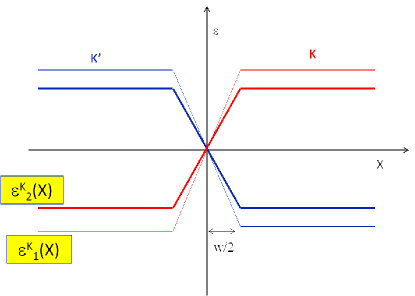
Figure 2: Quantum Hall energy spectrum of a double gated BLG, as a function of guiding center. We assume a smooth change in bias across $x=0$, and it yields the existence of zero energy states at $V=0$.

As shown in Eqs. (3) and (4), the energy eigenvalues $\varepsilon_{i}^{\mathbf{K}}(X)$ and $\varepsilon_{i}^{\mathbf{K^{\prime}}}(X)$ are determined by the profile of $V(X)$. They all vanish at $X=0$ where there is a level crossing between the $\mathbf{K}$ and $\mathbf{K^{\prime}}$ states. We thus find that the noninteracting ground state of undoped BLG possesses two pairs of “helical” edge states with opposite chiralities from different valleys. The ground state is characterized by a sharp valley domain wall around $x=0$, i.e. at zero bias.

III Interaction-induced valley kink: Hartree-Fock treatment

When the Coulomb interaction is incorporated, the system develops a ferromagnetic nature.Fertig et al. (1994) A sharp domain wall between two spin states or two valleys, as obtained in the non-interacting ground-state described above, is not energetically favorable due to its large cost in exchange energy. The competition between the single-particle energy and the exchange energy gives rise to a lower energy state: a smooth kink in the spin/valley degrees of freedom.

We focus on the situation shown in the center of Fig. 2, where below the Fermi surface the filled energy states on the left are dominated by the $\mathbf{K}$ valley, and on the right by the $\mathbf{K^{\prime}}$ valley. The Coulomb interaction modifies the sharp domain wall to a smooth valley kink which can be described by a trial wavefunction of the formFertig and Brey (2006)

$$\left|\Psi\right\rangle=\prod_{X}\left(\cos\frac{\theta(X)}{2}C_{\mathbf{K}X}^{\dagger}+\sin\frac{\theta(X)}{2}e^{i\varphi}C_{\mathbf{K^{\prime}}X}^{\dagger}\right)\left|0\right\rangle.$$ (7)

Here $C_{\mathbf{K}X}^{\dagger}$ and $C_{\mathbf{K^{\prime}}X}^{\dagger}$ create electrons in the levels $\varepsilon_{2}^{\mathbf{K}}(X)$ and $\varepsilon_{2}^{\mathbf{K^{\prime}}}(X)$ respectively, which are closest to the Fermi energy, and we assume that the $\varepsilon_{1}$ states are pushed farther away from the Fermi level when the Coulomb interaction is included. $\left|0\right\rangle$ denotes the vacuum state where all lower states of negative single-particle energy are occupied, and $\varphi$ is a constant parameter. The function $\theta(X)$ defines the valley profile of the domain wall varying from $0$ to $\pi$: as shown on the far left of Fig. 2, the filled state below the Fermi level is the $\mathbf{K}$ valley state which corresponds to $\theta=0$; likewise on the far right of the figure, the filled state below the Fermi level is the $\mathbf{K^{\prime}}$ which corresponds to $\theta=\pi$. Eq. (7) may be regarded as a restricted Hartree-Fock approximation to the groundstate. In the following, we use this to study the guiding center dependence of $\theta(X)$, and determine the width of the domain wall.

The total Hamiltonian of the interacting electron system is

$$H=H_{0}+H_{int},$$ (8)

with single particle energy

$$H_{0}={\displaystyle{\displaystyle\sum_{\tau X}\varepsilon_{\tau X}C_{\tau X}^{\dagger}C_{\tau X}}}$$ (9)

and interaction

$$H_{int}=\frac{1}{2}\int\mathtt{d}\mathbf{r}\mathtt{d}\mathbf{r^{\prime}}:\rho(\mathbf{r})V(\mathbf{r}-\mathbf{r^{\prime}})\rho(\mathbf{r^{\prime}}):.$$ (10)

Here $:(\cdot\cdot\cdot):$ indicates normal ordering. The density operator is projected into the two states closest to the Fermi energy,

$$\rho(\mathbf{r})={\textstyle{\displaystyle\sum_{\tau,\tau^{\prime},X,X^{\prime}}{\displaystyle\phi_{\tau^{\prime}X^{\prime}}^{*}(\mathbf{r})\phi_{\tau X}(\mathbf{r})C_{\tau^{\prime}X^{\prime}}^{\dagger}C_{\tau X},}}}$$ (11)

with $\phi$ as defined in Eq. (6), $\tau^{(^{\prime})}$ represents the valley index $\mathbf{K}$ and $\mathbf{K^{\prime}}$, and $V(\mathbf{r}-\mathbf{r^{\prime}})=\frac{e^{2}}{\kappa l_{B}\left|\mathbf{r}-\mathbf{r^{\prime}}\right|}$ is the Coulomb interaction among the electrons ($\kappa\sim 5.2$ for a suspended bilayer graphene).Gonzalez et al. (1999); Ghahari et al. (2011) We apply the Hartree-Fock approximation to the total Hamiltonian in Eq. (8) and evaluate expectation values in the ground state given by Eq. (7). The total Hamiltonian can therefore be written as $H={\displaystyle{\textstyle\sum_{X}}H_{X}^{HF}}$, where $H_{X}^{HF}$ is an effective $2\times 2$ Hamiltonian for each guiding center coordinate in the basis of $\left|\mathbf{K}X\right\rangle$ and $\left|\mathbf{K^{\prime}}X\right\rangle$,

$$H_{X}^{HF}=\left[\begin{array}[]{cc}\left(\varepsilon_{\mathbf{K}X}+J_{\mathbf{K}X,\mathbf{K}X}\right)&J_{\mathbf{K}X,\mathbf{K^{\prime}}X}\\ J_{\mathbf{K}X,\mathbf{K^{\prime}}X}^{*}&\left(\varepsilon_{\mathbf{K^{\prime}}X}+J_{\mathbf{K^{\prime}}X,\mathbf{K^{\prime}}X}\right)\end{array}\right].$$ (12)

Here $\varepsilon_{\mathbf{K^{\prime}}X}=-\varepsilon_{\mathbf{K}X}$ denote the single particle energies given by Eq. (4), and the interaction terms are

$$J_{\mathbf{K}X,\mathbf{K}X} = E_{H}-\frac{1}{2}\sum_{X^{\prime}}\left\langle C_{\mathbf{K}X^{\prime}}^{\dagger}C_{\mathbf{K}X^{\prime}}\right\rangle V_{X,X^{\prime}},$$ (13)

$$J_{\mathbf{K^{\prime}}X,\mathbf{K^{\prime}}X} = E_{H}-\frac{1}{2}\sum_{X^{\prime}}\left\langle C_{\mathbf{K^{\prime}}X^{\prime}}^{\dagger}C_{\mathbf{K^{\prime}}X^{\prime}}\right\rangle V_{X,X^{\prime}},$$ (14)

$$J_{\mathbf{K}X,\mathbf{K^{\prime}}X} = -\frac{e^{i\varphi}}{2}\sum_{X^{\prime}}\left\langle C_{\mathbf{K^{\prime}}X^{\prime}}^{\dagger}C_{\mathbf{K}X^{\prime}}\right\rangle V_{X,X^{\prime}},$$ (15)

in which

$$\left\langle C_{\mathbf{K}X^{\prime}}^{\dagger}C_{\mathbf{K}X^{\prime}}\right\rangle=\cos^{2}\frac{\theta(X^{\prime})}{2},$$

$$\left\langle C_{\mathbf{K^{\prime}}X^{\prime}}^{\dagger}C_{\mathbf{K^{\prime}}X^{\prime}}\right\rangle=\sin^{2}\frac{\theta(X^{\prime})}{2},$$

$$\left\langle C_{\mathbf{K^{\prime}}X^{\prime}}^{\dagger}C_{\mathbf{K}X^{\prime}}\right\rangle=\cos\frac{\theta(X^{\prime})}{2}\sin\frac{\theta(X^{\prime})}{2}.$$

$E_{H}=\sum_{X^{\prime}}V_{X^{\prime},X,X,X^{\prime}}$, where the integral $V_{X_{1},X_{2},X_{3},X_{4}}$ is defined in Eqs. (31) and (32-35), denotes the Hartree contribution to the single particle energies. Although $E_{H}$ is formally divergent, in practice it is canceled by interactions with a uniform neutralizing background, which is not explicitly included in our Hamiltonian. The exchange interaction matrix element $V_{X,X^{\prime}}\equiv V_{X^{\prime},X,X^{\prime},X}$ is given by

$$V_{X,X^{\prime}}=\frac{V_{0}}{L_{y}}e^{-\frac{\left(X-X^{\prime}\right)^{2}}{4}}\left\{U_{0}(X-X^{\prime})K_{0}\left[\frac{\left(X-X^{\prime}\right)^{2}}{4}\right]+U_{1}(X-X^{\prime})K_{1}\left[\frac{\left(X-X^{\prime}\right)^{2}}{4}\right]\right\},$$ (16)

where $V_{0}=\frac{e^{2}}{32\kappa l_{B}N_{h}^{4}}$, $K_{n}$ are the modified Bessel functions which are localized at $\left|X-X^{\prime}\right|<1$ , and $U_{0,1}$ denote polynomial functions of $\left(X-X^{\prime}\right)$ as described in Appendix A.

As shown in Eq. (12), the Coulomb interaction introduces off-diagonal exchange terms which open a gap, and yields a smooth domain wall as described by Eq. (7). The trial wavefunction $\left|\Psi\right\rangle$ obeys the eigenvalue equation

$$H_{X}^{HF}\left|\Psi\right\rangle=\varepsilon\left|\Psi\right\rangle.$$

Using Eqs. (7) and (12), this yields

$$\left[\begin{array}[]{cc}\left(\varepsilon_{\mathbf{K}X}+B_{X}\right)&\triangle_{X}\\ \triangle_{X}^{*}&-\left(\varepsilon_{\mathbf{K}X}+B_{X}\right)\end{array}\right]\left[\begin{array}[]{c}\cos\frac{\theta(X)}{2}\\ \sin\frac{\theta(X)}{2}\end{array}\right]=\left(\varepsilon-A\right)\left[\begin{array}[]{c}\cos\frac{\theta(X)}{2}\\ \sin\frac{\theta(X)}{2}\end{array}\right],$$ (17)

where we define

$$\triangle_{X} = J_{\mathbf{K}X,\mathbf{K^{\prime}}X},$$

$$A = E_{H}+\frac{1}{2}\left(J_{\mathbf{K}X,\mathbf{K}X}+J_{\mathbf{K^{\prime}}X,\mathbf{K^{\prime}}X}\right),$$

$$B_{X} = \frac{1}{2}\left(J_{\mathbf{K}X,\mathbf{K}X}-J_{\mathbf{K^{\prime}}X,\mathbf{K^{\prime}}X}\right).$$

This yields the relation

$$\left|\triangle_{X}\right|=\left(\varepsilon_{\mathbf{K}X}+B_{X}\right)\tan\theta(X),$$ (18)

and consequently

$$\sin\theta(X)=\frac{\left|\triangle_{X}\right|}{\sqrt{\left|\triangle_{X}\right|^{2}+\left(\varepsilon_{\mathbf{K}X}+B_{X}\right)^{2}}}$$ (19)

and

$$\cos\theta(X)=\frac{\left(\varepsilon_{\mathbf{K}X}+B_{X}\right)}{\sqrt{\left|\triangle_{X}\right|^{2}+\left(\varepsilon_{\mathbf{K}X}+B_{X}\right)^{2}}}.$$ (20)

The quantities $\left|\triangle_{X}\right|$ and $B_{X}$ must be determined self-consistently.

Using Eq. (19) for $\sin\theta(X)$ in Eq. (15) and replacing the sums over $X^{\prime}$ by integrals, we obtain two coupled gap equations,

$$\left|\triangle_{X}\right|=-\frac{L_{y}}{4\pi}\int\mathtt{d}X^{\prime}\frac{\left|\triangle_{X^{\prime}}\right|}{\sqrt{\left|\triangle_{X^{\prime}}\right|^{2}+\left(\varepsilon_{\mathbf{K}X^{\prime}}+B_{X^{\prime}}\right)^{2}}}V_{X,X^{\prime}},$$ (21)

$$B_{X}=-\frac{L_{y}}{4\pi}\int\mathtt{d}X^{\prime}\frac{\varepsilon_{\mathbf{K}X^{\prime}}+B_{X^{\prime}}}{\sqrt{\left|\triangle_{X^{\prime}}\right|^{2}+\left(\varepsilon_{\mathbf{K}X^{\prime}}+B_{X^{\prime}}\right)^{2}}}V_{X,X^{\prime}}.$$ (22)

When $X$ is near the center (i.e. $X\ll w$), we can assume $\triangle_{X^{\prime}}\sim\triangle_{X}$ and $B_{X}\sim B_{X^{\prime}}$. Since $\triangle_{X}\left(\triangle_{X}\neq 0\right)$ is maximum at $X=0$, and $B_{X}\rightarrow 0$ at $X=0$, an approximate solution to the gap equations takes the form

$$\triangle_{X}\approx\sqrt{\triangle_{0}^{2}-\left(\eta X+B_{X}\right)^{2},}$$ (23)

where

$$\triangle_{0}=V_{0}\sqrt{\frac{\pi}{8}}\left(8+8\beta^{2}+3\beta^{4}\right),$$

with $\beta=-\gamma_{1}/\omega_{c}$, and

$$\eta=\frac{\left(\gamma_{1}^{2}-\omega_{c}^{2}\right)V}{\left(\gamma_{1}^{2}+\omega_{c}^{2}\right)w},$$

which is the effective slope of the position dependent perpendicular bias;

$$B_{X} \sim -\frac{\eta}{\left(1+f(\beta)\right)}X,$$ (24)

with $f(\beta)=\left(8+8\beta^{2}+3\beta^{4}\right)/\left(8+8\beta^{2}+6\beta^{4}\right)$.

Combining Eqs. (23) and (24), we obtain

$$\left|\triangle_{X}\right|\sim\sqrt{\triangle_{0}^{2}-\eta^{2}\left(1-\frac{1}{1+f(\beta)}\right)^{2}X^{2}}.$$ (25)

Substituting this into Eq. (18), this yields an expression for $\theta(X)$. In Fig. 3 we plot this for sample parameters as listed in the caption of the figure. The width of the valley domain wall may be estimated to be

$$d_{DW}\sim\frac{\triangle_{0}}{\eta}\sim\frac{\triangle_{0}}{V}w$$

which is in general dependent on the ratio of the maximal Coulomb gap $\triangle_{0}$ (which has magnetic field dependence) to the applied bias and the separation of the two opposing polarity gates. $\theta(X)$ is almost linear in $X$ at the center and curves up on the sides where the approximations of $\triangle_{X^{\prime}}\sim\triangle_{X}$ and $B_{X}\sim B_{X^{\prime}}$ are no longer valid. It is apparent that the width of the kink can be tuned by the interplay between the magnetic field and gate electric fields. We expect that an exact minimization of the trial wavefunction would yield a very similar result near the center of the DW, but the singularities in the slopes near the edges would be smoothed out.

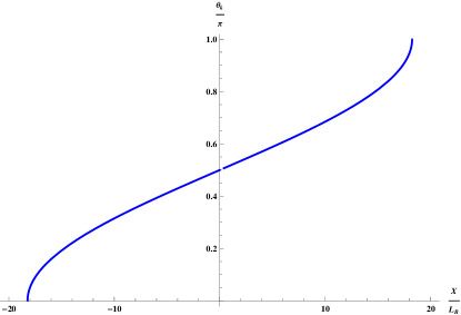
Figure 3: The guiding center dependence of $\theta$. The parameters are chosen as follows: $V=200$ meV, $l_{B}=10$ nm, $w=20\>l_{B}$, $\gamma_{1}/\omega_{c}=3$.

IV Interlayer charge density pattern

Here we propose a possible measurement to visualize the valley-kink domain wall derived in the previous section. We start by projecting the density operator of bilayer graphene into its four sublattices, i.e. $\rho(\mathbf{r})={\displaystyle\sum_{\mu}\rho_{\mu}(\mathbf{r})},$ where

$$\rho_{\mu}(\mathbf{r})={\displaystyle\sum_{\tau,\tau^{\prime}X,X^{\prime}}\phi_{\mu\tau X}^{*}(\mathbf{r})\phi_{\mu\tau^{\prime}X^{\prime}}(\mathbf{r})C_{\tau X}^{\dagger}C_{\tau^{\prime}X}}$$

in which $\mu$ represents the four sublattices $A$, $B$, $\tilde{A}$, and $\tilde{B}$, and $\phi_{\mu}$ represents the $\mu$th component of $\phi_{\mathbf{K}X}$ defined in Eq. (6).

Using Eq. (7), the expectation value of the density on sublattice $\mu$ is

$$\left\langle\rho_{\mu}(\mathbf{r})\right\rangle = \left\langle\Psi\right|\rho_{\mu}(\mathbf{r})\left|\Psi\right\rangle$$

$$= {\displaystyle\sum_{X}\cos^{2}\frac{\theta(X)}{2}R_{\mathbf{KK}X}^{\mu}(\mathbf{r})+\sin^{2}\frac{\theta(X)}{2}R_{\mathbf{K^{\prime}K^{\prime}}X}^{\mu}(\mathbf{r})}$$

$$+e^{i\varphi}\cos\frac{\theta(X)}{2}\sin\frac{\theta(X)}{2}\left[R_{\mathbf{KK^{\prime}}X}^{\mu}(\mathbf{r})+R_{\mathbf{K^{\prime}K}X}^{\mu}(\mathbf{r})\right],$$

where

$$R_{\tau\tau^{\prime}X}^{\mu}(\mathbf{r})=\phi_{\mu\tau X}^{*}(\mathbf{r})\phi_{\mu\tau^{\prime}X}(\mathbf{r}).$$

The last term of Eq. (IV) indicates interference between the $\mathbf{K}$ and $\mathbf{K^{\prime}}$ valleys. In the valley transition region, an interference pattern would therefore be manifested by the charge density difference between the top ($t$) and the bottom ($b$) layer of the BLG,

$$\triangle\rho(x,y) = \rho_{t}-\rho_{b},$$ (27)

$$= \left(\rho_{A}(\mathbf{r})+\rho_{B}(\mathbf{r})\right)-\left(\rho_{\tilde{A}}(\mathbf{r})+\rho_{\tilde{B}}(\mathbf{r})\right),$$

$$= \rho_{0}(x)+\rho_{CDW}(x)\cos\left(\Delta\mathbf{K}y+\varphi\right).$$ (28)

Here

$$\rho_{0}(x) = \frac{1}{N_{h}^{2}}\sum_{X}\cos\theta(X)\times$$

$$\left\{\beta^{2}\Phi_{1}^{2}(x-X)-\left[1-\alpha(X)^{2}\right]\Phi_{0}^{2}(x-X)\right\},$$

$$\rho_{CDW}(x)=\frac{4\gamma_{1}V}{N_{h}^{2}\left(\gamma_{1}^{2}+\omega_{c}^{2}\right)w}\sum_{X}X\Phi_{0}^{2}(x-X)\sin\theta(X),$$ (30)

with $\triangle\mathbf{K}=\mathbf{K}-\mathbf{K^{\prime}}$,

$$\alpha(X)=\frac{2\gamma_{1}VX}{\left(\gamma_{1}^{2}+\omega_{c}^{2}\right)w},$$

and the normalization factor $N_{h}\sim\sqrt{1+\beta^{2}}$. The first term in Eq. (28) represents the average charge density difference between the top and the bottom layers, while the second term describes a charge density wave through which we see a rapid oscillation along the $y$ direction with wave vector $\triangle\mathbf{K}$. The resulting interlayer charge density pattern is shown in Fig. 4, wherein the upper panel displays an intervalley interference along the $y$ direction and a dipolar charge profile along the $x$ direction. Across $x=0$, the interlayer charge density pattern shows an interesting antisymmetric amplitude which is due to the switch in polarity of the potential profile.

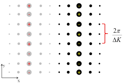
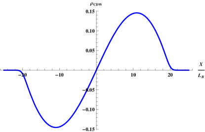
Figure 4: Interlayer charge density pattern in a BLG domain wall. Upper panel: a rapid oscillation along the y direction with wave vector $\triangle\mathbf{K}=\mathbf{K}-\mathbf{K^{\prime}}$, and a dipolar profile along the $x$ direction. Lower panel: at $y=0$ , the interlayer charge density pattern $\rho_{CDW}(x,0)$ the thick blue curve is obtained from numerical integral. The parameters chosen here are: $V=200$ meV, $l_{B}=10$ nm, $w=20\>l_{B}$, $\gamma_{1}/\omega_{c}=3$, $\varphi=0$.

V Concluding remarks

We have proposed an experimental setup to realize a collective, smooth kink in the valley degrees of freedom for bilayer graphene at $\nu=0$ in the presence of a spatially antisymmetric bias field. The width of the kink is determined by an interplay between the magnetic field and the gate electric fields. We predict a potentially measurable interlayer charge density pattern to visualize this resulting electronic structure. According to Eq. (30), the amplitude of the charge density pattern can be tuned by the ratio of $V$ to $\gamma_{1}$. This pattern is possibly accessible to measurement, e.g. by an STM probe.

The above results assume that the Zeeman splitting of the real spin is negligibly small compared to the maximal valley splitting set by the gate voltage. We note that for sufficiently strong magnetic fields where the real spin is resolved, two distinct crossing points appear in the non-interacting spectrum at zero energy, separated by a finite distance in real space. Consequently, a more complex double-kink pattern is expected to form in the interacting groundstate, which can be viewed as a pair of DW’s with a mutual interaction which is tunable by the gate-voltage. This case will be studied elsewhere.Hua

We conclude with speculations about the collective electronic transport behavior of this system. In analogy with what happens with a spin DW at the edge of single layer graphene at $\nu=0$,Fertig and Brey (2006); Shimshoni et al. (2009) we expect the DW to carry valley currents which can lead to a valley QHE. Unlike the single layer case, the non-interacting energy spectrum for the bilayer structure we consider has two pairs of states crossing the Fermi level, although one has much greater slope than the other. For long length scales, and for the purposes of static properties, in a first approximation one may ignore the higher energy states as we have done in this study. However, very close to $x=0$ the second pair of internal edge states will likely give the charge density profile further structure as they approach zero energy. More importantly, these extra states crossing the Fermi energy open a second current-carrying channel, which will affect the transport properties of the system. An interesting set of questions in this regard is how the second channel couples to the first, in particular if they can be regarded as independent channels or if they are locked together by Coulomb interactions. Finally, we note that in the case where the splitting of real-spin is appreciable, the two coupled DWs are likely to support a quasi 1D collective mode characterized by a ladder-like dynamics. We leave these questions for future research.

Appendix A Evaluation of the coulomb integrals

Using Eqs. (5) and (6) we write the Coulomb integral as follows:

$$V_{X_{1},X_{2},X_{3},X_{4}}=C_{1}V^{(1)}+C_{2}V^{(2)}+C_{3}\left(V^{(3)}+V^{(4)}\right),$$ (31)

where up to corrections of order $(V/\gamma_{1})^{2}$

$$C_{1} \approx \frac{e^{2}}{L_{y}^{2}\kappa l_{B}N_{h}^{4}},$$

$$C_{2} \approx \frac{e^{2}\beta^{4}}{L_{y}^{2}\kappa l_{B}N_{h}^{4}},$$

$$C_{3} \approx \frac{e^{2}\beta^{2}}{L_{y}^{2}\kappa l_{B}N_{h}^{4}},$$

with $\beta=-\gamma_{1}/\omega_{c}$, and

$$V^{(1)} = \int\mathtt{d}\mathbf{r}\mathtt{d}\mathbf{r^{\prime}}e^{i\left(X_{2}-X_{1}\right)\left(y-y^{\prime}\right)}\Phi_{0}^{*}(x-X_{1})\Phi_{0}^{*}(x^{\prime}-X_{2})V(\mathbf{r}-\mathbf{r^{\prime}})\Phi_{0}(x^{\prime}-X_{3})\Phi_{0}(x-X_{4}),$$ (32)

$$V^{(2)} = \int\mathtt{d}\mathbf{r}\mathtt{d}\mathbf{r^{\prime}}e^{i\left(X_{2}-X_{1}\right)\left(y-y^{\prime}\right)}\Phi_{1}^{*}(x-X_{1})\Phi_{1}^{*}(x^{\prime}-X_{2})V(\mathbf{r}-\mathbf{r^{\prime}})\Phi_{1}(x^{\prime}-X_{3})\Phi_{1}(x-X_{4}),$$ (33)

$$V^{(3)} = \int\mathtt{d}\mathbf{r}\mathtt{d}\mathbf{r^{\prime}}e^{i\left(X_{2}-X_{1}\right)\left(y-y^{\prime}\right)}\Phi_{0}^{*}(x-X_{1})\Phi_{1}^{*}(x^{\prime}-X_{2})V(\mathbf{r}-\mathbf{r^{\prime}})\Phi_{1}(x^{\prime}-X_{3})\Phi_{0}(x-X_{4}),$$ (34)

$$V^{(4)} = \int\mathtt{d}\mathbf{r}\mathtt{d}\mathbf{r^{\prime}}e^{i\left(X_{2}-X_{1}\right)\left(y-y^{\prime}\right)}\Phi_{1}^{*}(x-X_{1})\Phi_{0}^{*}(x^{\prime}-X_{2})V(\mathbf{r}-\mathbf{r^{\prime}})\Phi_{0}(x^{\prime}-X_{3})\Phi_{1}(x-X_{4}).$$ (35)

In particular, for $X_{1}=X_{3}=X^{\prime}$ and $X_{2}=X_{4}=X$ this yields the exchange interaction terms $V_{X,X^{\prime}}$. As an example, Eq. (32) may be written explicitly in the form

$$V^{(1)} = \frac{1}{\pi}\int\mathtt{d^{2}}r\mathtt{d^{2}}r^{\prime}e^{i\left(X-X^{\prime}\right)\left(y-y^{\prime}\right)}\frac{\exp\left\{-\frac{1}{2}\left[\left(x-X\right)^{2}+\left(x^{\prime}-X^{\prime}\right)^{2}+\left(x^{\prime}-X\right)^{2}+\left(x-X^{\prime}\right)^{2}\right]\right\}}{\sqrt{\left(x-x^{\prime}\right)^{2}+\left(y-y^{\prime}\right)^{2}}}.$$

To evaluate this, we change variables to difference and center coordinates $\tilde{x}=\left(x-x^{\prime}\right)$, $\tilde{y}=y-y^{\prime}$, $x_{c}=\frac{\left(x+x^{\prime}\right)}{2}$, and $y_{c}=\frac{\left(y+y^{\prime}\right)}{2}$, and first integrate over $x_{c}$ and $y_{c}$, to obtain

$$V^{(1)}=\frac{L_{y}\sqrt{2\pi}}{4\pi}e^{-\frac{\left(X-X^{\prime}\right)^{2}}{2}}\int\mathtt{d}\tilde{x}\mathtt{d}\tilde{y}\frac{e^{i\left(X-X^{\prime}\right)\tilde{y}}e^{-\frac{\tilde{x}^{2}}{2}}}{\sqrt{\tilde{x}^{2}+\tilde{y}^{2}}}.$$ (36)

We then use the 2D Fourier transform of the Coulomb potential

$$\frac{1}{\sqrt{\tilde{x}^{2}+\tilde{y}^{2}}} = \frac{1}{2\pi}\int\mathtt{d}^{2}k_{2}\frac{e^{-i\mathbf{k_{2}}\cdot\triangle\mathbf{r}}}{k_{2}},$$ (37)

to obtainJeffrey and Zwillinger (2007)

$$V^{(1)} = \frac{L_{y}}{2}e^{-\frac{\left(X-X^{\prime}\right)^{2}}{2}}\int\mathtt{d}k_{2x}\frac{e^{-\frac{k_{2x}^{2}}{2}}}{\sqrt{k_{2x}^{2}+\left(X-X^{\prime}\right)^{2}}},$$ (38)

$$= \frac{L_{y}}{2}e^{-\frac{\left(X-X^{\prime}\right)^{2}}{4}}K_{0}\left[\frac{\left(X-X^{\prime}\right)^{2}}{4}\right].$$

Similarly we can evaluate $V^{(2)}$, $V^{(3)}$, and $V^{(4)}$ and obtain the final expression for the Coulomb integral in Eq. (16), with

$$U_{0}(X-X^{\prime}) = \beta^{4}\left[\left(X-X^{\prime}\right)^{4}-4\left(X-X^{\prime}\right)^{2}+8\right]-4\beta^{2}\left[\left(X-X^{\prime}\right)^{2}-4\right]+8,$$ (39)

$$U_{1}(X-X^{\prime}) = \beta^{2}\left(X-X^{\prime}\right)^{2}\left\{\beta^{2}\left[\left(X-X^{\prime}\right)^{2}-2\right]-4\right\}.$$ (40)

References

• Sarma and Pinczuk (1997) S. D. Sarma and A. Pinczuk, eds., Perspectives in Quantum Hall Effects (John Wiley & Sons, INC., 1997).
• Prange and Girvin (1990) R. Prange and S. M. Girvin, eds., The Quantum Hall Effect (Springer-Verlag, New York, 1990).
• Sondhi et al. (1993) S. L. Sondhi, A. Karlhede, S. A. Kivelson, and E. H. Rezayi, Phys. Rev. B 47, 16419 (1993).
• Fertig et al. (1994) H. A. Fertig, L. Brey, R. Cote, and A. H. MacDonald, Phys. Rev. B 50, 11018 (1994).
• Moon et al. (1995) K. Moon, H. Mori, K. Yang, S. M. Girvin, A. H. MacDonald, L. Zheng, D. Yoshioka, and S.-C. Zhang, Phys. Rev. B 51, 5138 (1995).
• Abanin et al. (2007) D. A. Abanin, K. S. Novoselov, U. Zeitler, P. A. Lee, A. K. Geim, and L. S. Levitov, Phys. Rev. Lett. 98, 196806 (2007).
• Bolotin et al. (2009) K. I. Bolotin, F. Ghahari, M. D. Shulman, H. L. Stormer, and P. Kim, Nature 462, 196 (2009), ISSN 0028-0836.
• Du et al. (2009) X. Du, I. Skachko, F. Duerr, A. Luican, and E. Y. Andrei, Nature 462, 192 (2009), ISSN 0028-0836.
• Fertig and Brey (2006) H. A. Fertig and L. Brey, Phys. Rev. Lett. 97, 116805 (2006).
• Zhao et al. (2010) Y. Zhao, P. Cadden-Zimansky, Z. Jiang, and P. Kim, Phys. Rev. Lett. 104, 066801 (2010).
• Barlas et al. (2008) Y. Barlas, R. Cote, K. Nomura, and A. H. MacDonald, Phys. Rev. Lett. 101, 097601 (2008).
• Cote et al. (2008) R. Cote, J.-F. Jobidon, and H. A. Fertig, Phys. Rev. B 78, 085309 (2008).
• Novoselov et al. (2005) K. S. Novoselov, A. K. Geim, S. V. Morozov, D. Jiang, M. I. Katsnelson, I. V. Grigorieva, S. V. Dubonos, and A. A. Firsov, Nature 438, 197 (2005), ISSN 0028-0836.
• Novoselov et al. (2006) K. S. Novoselov, E. McCann, S. V. Morozov, V. I. Fallko, M. I. Katsnelson, U. Zeitler, D. Jiang, F. Schedin, and A. K. Geim, Nat Phys 2, 177 (2006), ISSN 1745-2473.
• Zhang et al. (2005) Y. Zhang, Y.-W. Tan, H. L. Stormer, and P. Kim, Nature 438, 201 (2005), ISSN 0028-0836.
• Zheng and Ando (2002) Y. Zheng and T. Ando, Phys. Rev. B 65, 245420 (2002).
• Zhang et al. (2006) Y. Zhang, Z. Jiang, J. P. Small, M. S. Purewal, Y.-W. Tan, M. Fazlollahi, J. D. Chudow, J. A. Jaszczak, H. L. Stormer, and P. Kim, Phys. Rev. Lett. 96, 136806 (2006).
• Zhao et al. (2012) Y. Zhao, P. Cadden-Zimansky, F. Ghahari, and P. Kim, arXive:1201.4434 (2012).
• Shimshoni et al. (2009) E. Shimshoni, H. A. Fertig, and G. V. Pai, Phys. Rev. Lett. 102, 206408 (2009).
• Castro Neto et al. (2006) A. H. Castro Neto, F. Guinea, and N. M. R. Peres, Phys. Rev. B 73, 205408 (2006).
• Brey and Fertig (2006) L. Brey and H. A. Fertig, Phys. Rev. B 73, 195408 (2006).
• Li et al. (2011) J. Li, I. Martin, M. Buttiker, and A. F. Morpurgo, Nat Phys 7, 38 (2011), ISSN 1745-2473.
• Martin et al. (2008) I. Martin, Y. M. Blanter, and A. F. Morpurgo, Phys. Rev. Lett. 100, 036804 (2008).
• Zarenia et al. (2011) M. Zarenia, J. M. Pereira, G. A. Farias, and F. M. Peeters, Phys. Rev. B 84, 125451 (2011).
• McCann and Falko (2006) E. McCann and V. I. Falko, Phys. Rev. Lett. 96, 086805 (2006).
• McCann (2006) E. McCann, Phys. Rev. B 74, 161403 (2006).
• Mazo et al. (2011) V. Mazo, E. Shimshoni, and H. A. Fertig, Phys. Rev. B 84, 045405 (2011).
• Castro Neto et al. (2009) A. H. Castro Neto, F. Guinea, N. M. R. Peres, K. S. Novoselov, and A. K. Geim, Rev. Mod. Phys. 81, 109 (2009).
• Wallace (1947) P. R. Wallace, Phys. Rev. 71, 622 (1947).
• Gonzalez et al. (1999) J. Gonzalez, F. Guinea, and M. A. H. Vozmediano, Phys. Rev. B 59, R2474 (1999).
• Ghahari et al. (2011) F. Ghahari, Y. Zhao, P. Cadden-Zimansky, K. Bolotin, and P. Kim, Phys. Rev. Lett. 106, 046801 (2011).
• (32) Chia-Wei Huang, H.A. Fertig, and E. Shimshoni, unpublished.
• Jeffrey and Zwillinger (2007) A. Jeffrey and D. Zwillinger, eds., Table of Integrals, Series and Products (Elsevier Academic Press publications, 2007).